Geometric Error Analysis of a 2UPR-RPU Over-Constrained Parallel Manipulator

Abstract

For a 2UPR-RPU over-constrained parallel manipulator, some geometric errors result in internal forces and deformations, which limit the improvement of the pose accuracy of the moving platform and shorten the service life of the manipulator. Analysis of these geometric errors is important for restricting them. In this study, an evaluation model is established to analyse the influence of geometric errors on the limbs’ comprehensive deformations for this manipulator. Firstly, the nominal inverse and actual forward kinematics are analysed according to the vector theory and the local product of the exponential formula. Secondly, the evaluation model of the limbs’ comprehensive deformations is established based on kinematics. Thirdly, 41 geometric errors causing internal forces and deformations are identified and the results are verified through simulations based on the evaluation model. Next, two global sensitivity indices are proposed and a sensitivity analysis is conducted using the Monte Carlo method throughout the reachable workspace of the manipulator. The results of the sensitivity analysis indicate that 10 geometric errors have no effects on the average angular comprehensive deformation and that the identified geometric errors have greater effects on the average linear comprehensive deformation. Therefore, the distribution of the global sensitivity index of the average linear comprehensive deformation is more meaningful for accuracy synthesis. Finally, simulations are performed to verify the results of sensitivity analysis.

1. Introduction

Parallel mechanisms with three DOFs have been successfully applied to hybrid serial–parallel machine tools, such as the well-known Eco-speed series, Tricept, and Exechon [1,2,3,4,5,6], owing to their high stiffness, large payload, and good dynamics. To achieve a simpler structure, Li et al. [3] designed a 2R1T (R denotes a rotational DOF, and T denotes a translational DOF) parallel mechanism named 2UPR-RPU. This mechanism is not only easier to control but also suitable for many operations along the surfaces. However, it is an over-constrained parallel mechanism with common constraints and over-constraints [7,8]. Some geometric errors in a manipulator based on this mechanism break the common constraints and over-constraints, resulting in internal forces and deformations. The internal forces and deformations not only limit the further improvement of the pose accuracy of the moving platform but also shorten the service life of the manipulator [9,10]. Therefore, it is necessary to restrict the internal-force-and-deformation-related geometric errors in the 2UPR-RPU parallel manipulator.

The accuracy design [11,12,13] can be applied to restrict geometric errors by determining the tolerances of the fabrication and assembly of machines. It consists of three components: error modelling [14,15,16], sensitivity analysis [17,18,19], and accuracy synthesis [20,21,22], where error modelling is the basis of sensitivity analysis and accuracy synthesis. Zhang et al. [13] applied the closed-loop vector and first-order perturbation methods to establish a geometric error model for a 2UPR-RPS over-constrained manipulator, and they identified the geometric errors that affected the pose errors of the moving platform. Zhang et al. [15] utilised the screw theory to establish a geometric error model for a 4RSR-SS over-constrained parallel tracking machine. With the use of the geometric error model, 53 geometric errors that had a significant influence on the pose errors of the moving platform were identified after sensitivity analysis. However, neither of the above two methods considers the deformations caused by internal forces in over-constrained parallel manipulators. Taking parameter uncertainties into account, Tang et al. [23] built a general interval kinetostatic model for a 2UPR-SPR over-constrained parallel machine to perform sensitivity analysis and tolerance allocation. To predict the pose errors of an over-constrained extendible support structure, Yu et al. [24] proposed a comprehensive model that simultaneously considered geometric errors, joint gaps, and link flexibility. In spite of good accuracy, these two models are complicated for the stiffness matrix needs to be derived and the stiffness coefficients of parts need to be obtained via finite element software.

Affected by geometric errors, the end poses of different limbs of a parallel manipulator should be theoretically inconsistent. However, they can be consistent in non-overconstrained parallel manipulators due to the existence of the moving platform and the motion deviations of passive joints. On this basis, a numerical iterative algorithm [25,26] was proposed to analyse the kinematics of non-overconstrained parallel manipulators with kinematic errors. Inspired by this algorithm, this study aims to establish an evaluation model based on kinematics to analyse the influence of geometric errors on the limbs’ comprehensive deformations for the 2UPR-RPU over-constrained parallel manipulator.

Based on the established evaluation model, sensitivity analysis can help reveal the influence of different internal-force-and-deformation-related geometric errors on the limbs’ comprehensive deformations. The interval analysis method and probabilistic method have been commonly used for sensitivity analysis of the moving platform’s pose error in literature. The interval analysis method treats geometric errors as interval variables and can get a balance between calculation speed and accuracy [11,18]. Treating geometric errors as random variables with a normal distribution, the probabilistic method can be divided into the Monte Carlo method and the probability modelling method. The Monte Carlo method calculates the moving platform’s pose errors according to the geometric error model and lots of random values of a geometric error [22,27]. It has good accuracy and low computational efficiency. The probability modelling method establishes an analytical model between the standard deviation of each geometric error and that of the moving platform’s pose error based on the geometric error model [28]. In spite of high computational efficiency, this method needs prior knowledge about probability distributions. Considering that the interval analysis method and probability modelling method are not suitable when the geometric error model is iterative, the Monte Carlo method is utilised to analyse the influence of geometric errors on the limbs’ comprehensive deformations in this paper.

The remainder of this paper is organised as follows. In Section 2, the 2UPR-RPU parallel mechanism is briefly introduced. Section 3 presents an analysis of the nominal inverse kinematics and actual forward kinematics. Section 4 establishes an evaluation model of the limbs’ comprehensive deformations caused by geometric errors. Based on the evaluation model, the internal-force-and-deformation-related geometric errors are identified and the results are verified through simulations in Section 5. In Section 6, two global sensitivity indices are proposed and sensitivity analysis is conducted. Simulations are also performed to verify the results of sensitivity analysis. Finally, the conclusions are drawn in Section 7.

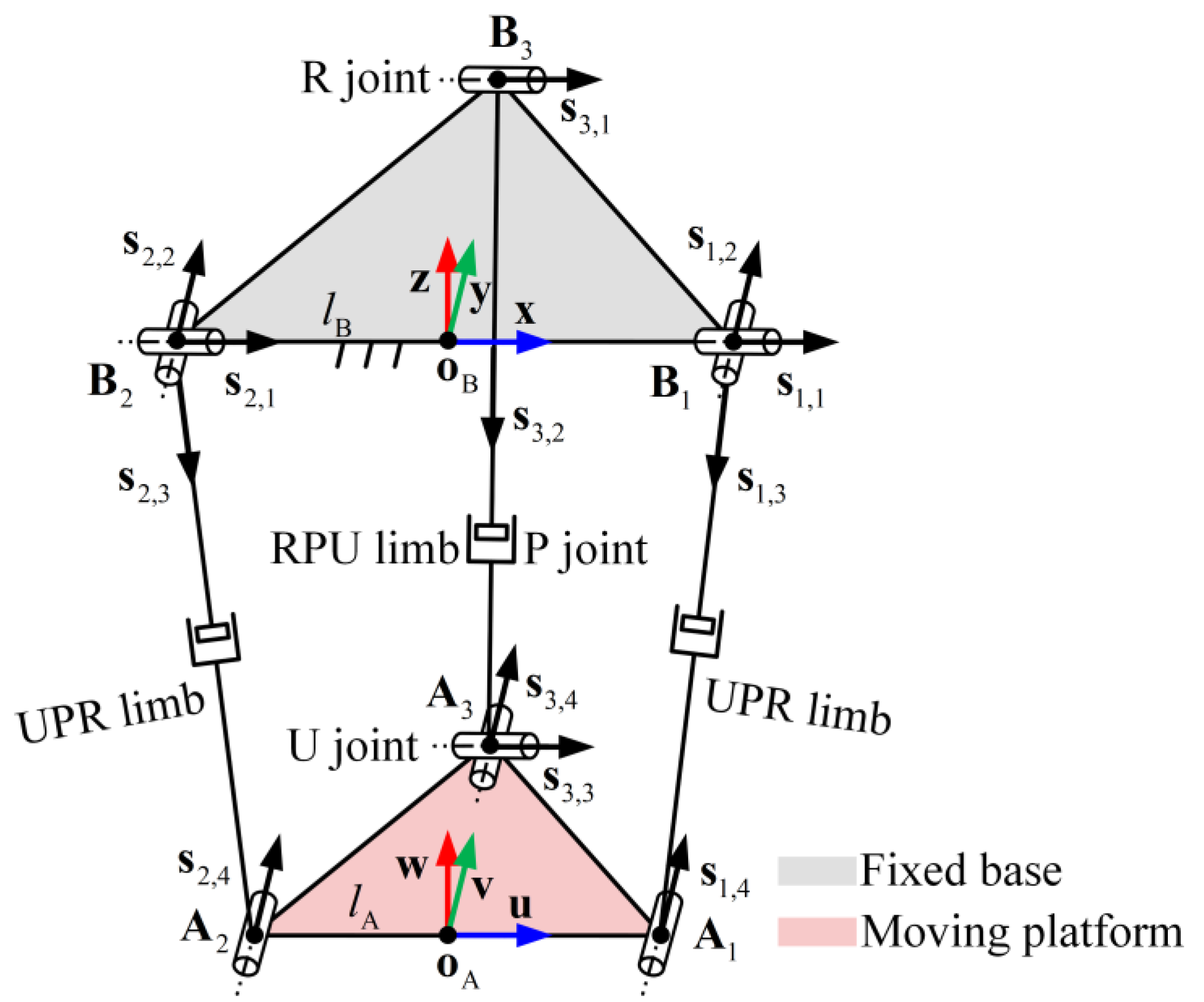
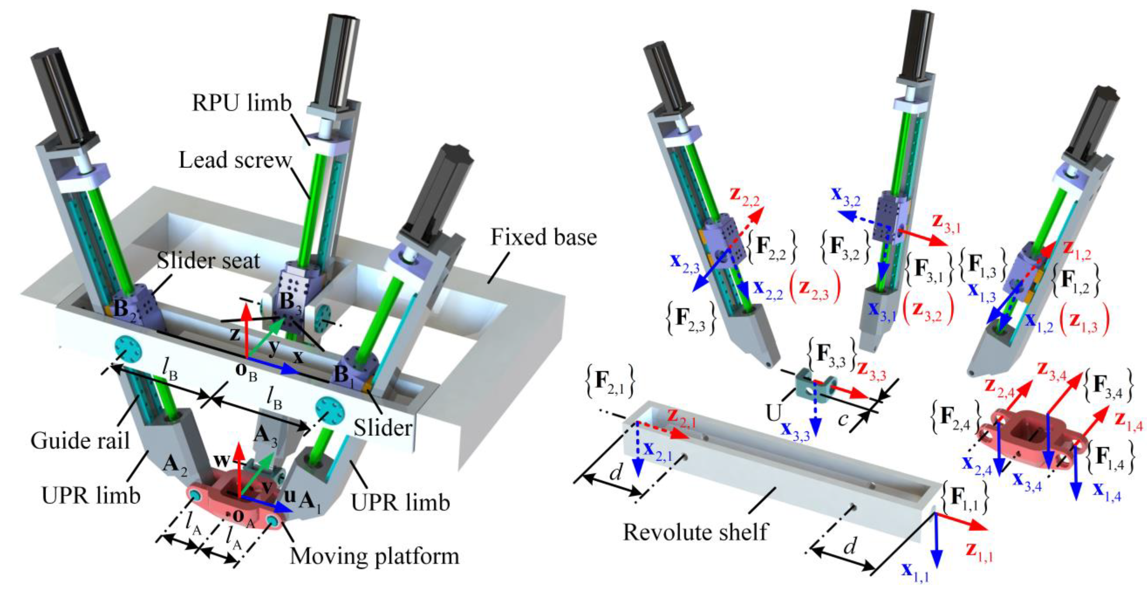
2. 2UPR-RPU Parallel Mechanism

As shown in Figure 1, the 2UPR-RPU parallel mechanism mainly consists of a moving platform, two UPR limbs, one RPU limb, and one fixed base, where the moving platform and fixed base are represented by the isosceles right triangles ΔA₁A₂A₃ and ΔB₁B₂B₃. U, P, and R denote universal, prismatic, and revolute joints, respectively. B₁, B₂ and A₃ are the centres of U, and A₁, A₂ and B₃ are the centres of R. Because each universal joint is equivalent to two mutually perpendicular revolute joints, the UPR limb is equivalent to the RRPR limb, and the RPU limb is equivalent to the RPRR limb. The axis of the jth joint of the ith limb is denoted by s_i,j. A fixed coordinate system {o_B; x, y, z} is established at the midpoint between B₁ and B₂, where x points from B₂ to B₁ and y points from o_B to B₃. Similarly, a moving coordinate system {o_A; u, v, w} is also established, where u points from A₂ to A₁ and v points from o_A to A₃. The coordinate axes z and w are determined using the right-hand rule. For the 2UPR-RPU parallel mechanism, each limb exerts a force and a couple on the moving platform [8], where the two forces from the UPR limbs are parallel to v, and the three couples from the UPR and RPU limbs rotate around w. It is worth mentioning that the two forces parallel to v will lead to over-constraint, and the three couples rotating around w will lead to common constraints. Thus, the 2UPR-RPU parallel mechanism is an over-constrained parallel mechanism.

3. Kinematics

Inverse kinematics aims to calculate the displacements of all joints relative to their initial positions or angles according to a given target pose of the moving platform. Forward kinematics is the reverse operation of inverse kinematics. Inverse kinematics without considering geometric errors is called nominal inverse kinematics. In this section, the nominal inverse kinematics of actuated joints and passive joints is first introduced. Then, the actual forward kinematics of the limbs is derived.

3.1. Nominal Inverse Kinematics

The position and orientation of the moving platform shown in Figure 1 can be described by ${\left[\begin{array}{ccc}x& y& z\end{array}\right]}^{\mathrm{T}}$ and ${\left[\begin{array}{ccc}\alpha & \beta & \gamma \end{array}\right]}^{\mathrm{T}}$, respectively, where ${\left[\begin{array}{ccc}x& y& z\end{array}\right]}^{\mathrm{T}}$ denotes the position coordinates of o_A with respect to {o_B; x, y, z} and ${\left[\begin{array}{ccc}\alpha & \beta & \gamma \end{array}\right]}^{\mathrm{T}}$ denotes the Euler angle with respect to z-x-v. Because only the translation motion along o_Bo_A and the rotations around x and v can be achieved by the moving platform [8], ${\left[\begin{array}{ccc}z& \beta & \gamma \end{array}\right]}^{\mathrm{T}}$ is sufficient to represent the poses. For a given target pose of the moving platform, the nominal displacements of actuated P-joints can be derived using the closed-loop vector method [10] as follows:

$$\{\begin{array}{l}{q}_{1,3}=\Vert B_1{A}_1\Vert -\Vert B_1{\tilde{A}}_1\Vert \hfill \\ q_{2,3}=\Vert B_2{A}_2\Vert -\Vert B_2{\tilde{A}}_2\Vert \hfill \\ q_{3,2}=\Vert B_3{A}_3\Vert -\Vert B_3{\tilde{A}}_3\Vert \hfill \end{array}$$

(1)

where $\Vert \cdot \Vert$ represents the Euclidean norm. ${\tilde{A}}_i$ denotes the initial position of A_i, which is determined by

$$\{\begin{array}{l}{B}_1{A}_1={\left[\begin{array}{ccc}{l}_{\mathrm{A}}\cos \gamma -l_{\mathrm{B}}& l_{\mathrm{A}}\sin \beta \sin \gamma -z\tan \beta & -l_{\mathrm{A}}\cos \beta \sin \gamma +z\end{array}\right]}^{\mathrm{T}}\hfill \\ B_2{A}_2={\left[-\begin{array}{ccc}{l}_{\mathrm{A}}\cos \gamma +l_{\mathrm{B}}& -l_{\mathrm{A}}\sin \beta \sin \gamma -z\tan \beta & l_{\mathrm{A}}\cos \beta \sin \gamma +z\end{array}\right]}^{\mathrm{T}}\hfill \\ B_3{A}_3={\left[\begin{array}{ccc}0& l_{\mathrm{A}}\cos \beta -z\tan \beta -l_{\mathrm{B}}& l_{\mathrm{A}}sin\beta +z\end{array}\right]}^{\mathrm{T}}\hfill \end{array}$$

(2)

where $l_{\mathrm{A}}=\Vert A_1{A}_2\Vert /2$ and $l_{\mathrm{B}}=\Vert B_1{B}_2\Vert /2$.

For the first UPR limb, the first, second, and fourth joints are passive. The nominal displacement of the first joint can be expressed as

$$q_{1,1}=\beta$$

(3)

The nominal displacement of the second joint can be expressed as

$$q_{1,2}=\arccos \left(\frac{e_1^{\mathrm{T}}{B}_1{A}_1}{\Vert B_1{A}_1\Vert }\right)-\arccos \left(\frac{e_1^{\mathrm{T}}{B}_1{\tilde{A}}_1}{\Vert B_1{\tilde{A}}_1\Vert }\right)$$

(4)

where e₁ is the unit vector along x.

The nominal displacement of the fourth joint can be expressed as

$$q_{1,4}=\arccos \left(\frac{-{\left(A_1{\tilde{A}}_2\right)}^{\mathrm{T}}\left(B_1{\tilde{A}}_1\right)}{\Vert A_1{\tilde{A}}_2\Vert \Vert B_1{\tilde{A}}_1\Vert }\right)-\arccos \left(\frac{-{\left(A_1{A}_2\right)}^{\mathrm{T}}\left(B_1{A}_1\right)}{\Vert A_1{A}_2\Vert \Vert B_1{A}_1\Vert }\right)$$

(5)

Because the two UPR limbs are symmetrically distributed with respect to o_Ao_B, we have

$$q_{2,1}=\beta$$

(6)

$$q_{2,2}=\arccos \left(\frac{e_1^{\mathrm{T}}{B}_2{A}_2}{\Vert B_2{A}_2\Vert }\right)-\arccos \left(\frac{e_1^{\mathrm{T}}{B}_2{\tilde{A}}_2}{\Vert B_2{\tilde{A}}_2\Vert }\right)$$

(7)

$$q_{2,4}=\arccos \left(\frac{{\left(A_1{A}_2\right)}^{\mathrm{T}}\left(B_2{A}_2\right)}{\Vert A_1{A}_2\Vert \Vert B_2{A}_2\Vert }\right)-\arccos \left(\frac{{\left(A_1{\tilde{A}}_2\right)}^{\mathrm{T}}\left(B_2{\tilde{A}}_2\right)}{\Vert A_1{\tilde{A}}_2\Vert \Vert B_2{\tilde{A}}_2\Vert }\right)$$

(8)

Similarly, the nominal displacements of the first, third, and fourth joints of the RPU limb can be expressed as

$$q_{3,1}=\arccos \left(\frac{-e_2^{\mathrm{T}}{B}_3{A}_3}{\Vert B_3{A}_3\Vert }\right)-\arccos \left(\frac{-e_2^{\mathrm{T}}{B}_3{\tilde{A}}_3}{\Vert B_3{\tilde{A}}_3\Vert }\right)$$

(9)

$$q_{3,3}=\arccos \left(\frac{{\left(R{e}_2\right)}^{\mathrm{T}}\left(B_3{A}_3\right)}{\Vert B_3{A}_3\Vert }\right)-\arccos \left(\frac{{\left(\tilde{R}{e}_2\right)}^{\mathrm{T}}\left(B_3{\tilde{A}}_3\right)}{\Vert B_3{\tilde{A}}_3\Vert }\right)$$

(10)

$$q_{3,4}=\gamma$$

(11)

Here, e₂ is the unit vector along y, and $\tilde{R}$ denotes the initial state of R, which is given as follows:

$$R=\left[\begin{array}{ccc}\cos \gamma & 0& \sin \gamma \\ \sin \beta \sin \gamma & \cos \beta & -\sin \beta \cos \gamma \\ -\cos \beta \sin \gamma & \sin \beta & \cos \beta \cos \gamma \end{array}\right]$$

(12)

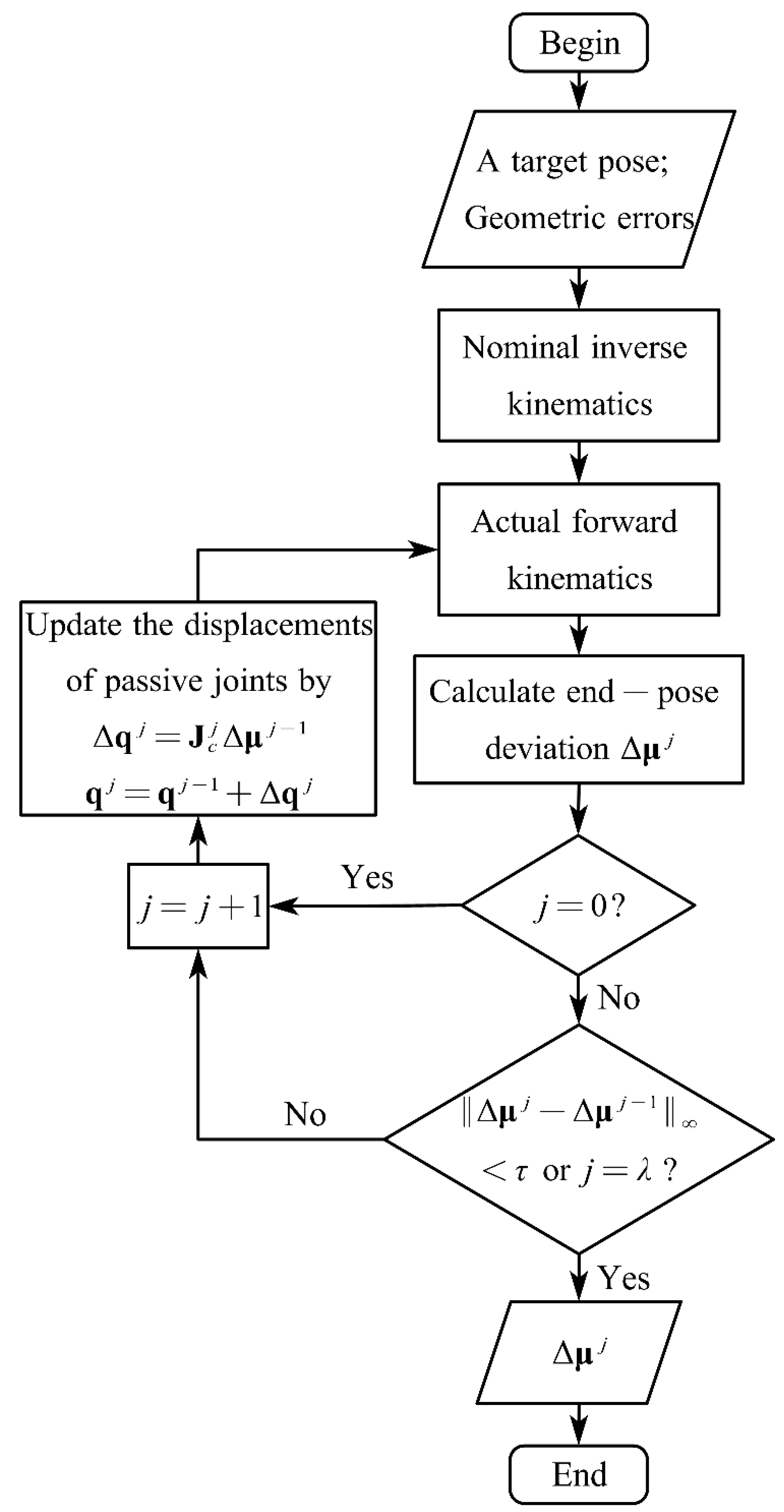
3.2. Actual Forward Kinematics

The nominal inverse kinematics described above does not consider geometric errors. However, geometric errors exist in the 2UPR-RPU parallel manipulator. In this section, the actual forward kinematics of the limbs in the manipulator is derived in detail.

As shown in Figure 2, four local coordinate systems {F_i,j; x_i,j, y_i,j, z_i,j} are assigned to each limb to describe the geometric errors of the 2UPR-RPU parallel manipulator, where the initial pose of the moving platform is ${\left[\begin{array}{ccc}{z}_0& {\beta }_0& {\gamma }_0\end{array}\right]}^{\mathrm{T}}={\left[\begin{array}{ccc}-0.2\mathrm{m}& 0& 0\end{array}\right]}^{\mathrm{T}}$ under the home configuration. The coordinate systems {o_B; x, y, z} and {o_A; u, v, w} are identical to those in Figure 1. For brevity, we use {F_i,j} instead of {F_i,j; x_i,j, y_i,j, z_i,j}. It is worth mentioning that this figure only shows x_i,j and z_i,j of the local coordinate systems, and y_i,j can be determined according to the right-hand rule, which will not be illustrated in detail here. The definitions of the local coordinate systems for the two UPR limbs and the RPU limb are listed in

Table 1. Definitions of local coordinate systems for the first UPR limb.

{Fi,j}	The Location	Fi,j	xi,j	zi,j
{F1,1}	On the revolute shelf	The intersection of the right hole axis of the revolute shelf and the right end face of the revolute shelf	Parallel to the intersection of the front and rear symmetry plane of the right hole of the revolute shelf and the vertical plane of the right hole axis	Coincide with the right hole axis of the revolute shelf
			Point down	Point outwards
{F1,2}	On the slider seat	The midpoint of the hole axis of the slider seat	Parallel to the intersection of the slider mounting plane and the vertical plane of the hole axis of the slider seat	Coincide with the hole axis of the slider seat
			Point to the moving platform	Point to the RPU limb
{F1,3}	On the lead screw	The intersection of the lead screw axis and the plane passing through z1,2 and perpendicular to the slider mounting plane	Parallel to the intersection of the guide rail plane and the vertical plane of the lead screw axis	Coincide with the lead screw axis
			Point in the direction opposite to the RPU limb	Point to the moving platform
{F1,4}	On the moving platform	The midpoint of the right hole axis of the moving platform	Parallel to the intersection of the vertical plane of the right hole axis of the moving platform and the plane constructed with v and w	Coincide with the right hole axis of the moving platform
			Point down	Point to the RPU limb

,

Table 2. Definitions of local coordinate systems for the second UPR limb.

{Fi,j}	The Location	Fi,j	xi,j	zi,j
{F2,1}	On the revolute shelf	The intersection of the left hole axis of the revolute shelf and the left end face of the revolute shelf	Parallel to the intersection of the front and rear symmetry plane of the left hole of the revolute shelf and the vertical plane of the left hole axis	Coincide with the left hole axis of the revolute shelf
			Point down	Point inwards
{F2,2}	On the slider seat	The midpoint of the hole axis of the slider seat	Parallel to the intersection of the slider mounting plane and the vertical plane of the hole axis of the slider seat	Coincide with the hole axis of the slider seat
			Point to the moving platform	Point to the RPU limb
{F2,3}	On the lead screw	The intersection of the lead screw axis and the plane passing through z2,2 and perpendicular to the slider mounting plane	Parallel to the intersection of the guide rail plane and the vertical plane of the lead screw axis	Coincide with the lead screw axis
			Point in the direction opposite to the RPU limb	Point to the moving platform
{F2,4}	On the moving platform	The midpoint of the left hole axis of the moving platform	Parallel to the intersection of the vertical plane of the left hole axis of the moving platform and the plane constructed with v and w	Coincide with the left hole axis of the moving platform
			Point down	Point to the RPU limb

and

Table 3. Definitions of local coordinate systems for the RPU limb.

{Fi,j}	The Location	Fi,j	xi,j	zi,j
{F3,1}	On the slider seat	The midpoint of the hole axis of the slider seat	Parallel to the intersection of the slider mounting plane and the vertical plane of the hole axis of the slider seat	Coincide with the hole axis of the slider seat
			Point to the moving platform	Point to the first UPR limb
{F3,2}	On the lead screw	The intersection of the lead screw axis and the plane passing through z3,1 and perpendicular to the slider mounting plane	Parallel to the intersection of the guide rail plane and the vertical plane of the lead screw axis	Coincide with the lead screw axis
			Point to the second UPR limb	Point to the moving platform
{F3,3}	On the U joint	The midpoint of the hole axis of the U joint	Parallel to the intersection of the vertical planes of the two hole axes of the U joint	Coincide with the hole axis of the U joint
			Point down	Point to the first UPR limb
{F3,4}	On the moving platform	The intersection of the rear hole axis of the moving platform and the rear end face of the moving platform	Parallel to the intersection of the vertical plane of the rear hole axis of the moving platform and the plane constructed with v and w	Coincide with the rear hole axis of the moving platform
			Point down	Point to the RPU limb

.

The end poses of the ith limb can be obtained from the local product of the exponential formula [25] as

$$g_i\left(q_i\right)=g_{i,0}{e}^{{\widehat{\zeta }}_{i,1}{q}_{i,1}}{g}_{i,1}{e}^{{\widehat{\zeta }}_{i,2}{q}_{i,2}}{g}_{i,2}{e}^{{\widehat{\zeta }}_{i,3}{q}_{i,3}}{g}_{i,3}{e}^{{\widehat{\zeta }}_{i,4}{q}_{i,4}}{g}_{i,4},i=1,2,3$$

(13)

where g_i denotes the homogeneous transformation matrix (HTM) of {o_A; u, v, w} with respect to {o_B; x, y, z} calculated using the ith limb. ζ_i,j denotes the screw coordinates of s_i,j with respect to {F_i,j}, which can be written as [25,26]

$$\{\begin{array}{c}{\zeta }_{i,j}={\left[\begin{array}{llllll}0\hfill & 0\hfill & 1\hfill & 0\hfill & 0\hfill & 0\hfill \end{array}\right]}^{\mathrm{T}} \mathrm{for} \mathrm{R} \mathrm{jo}\mathrm{int}\\ {\zeta }_{i,j}={\left[\begin{array}{llllll}0\hfill & 0\hfill & 0\hfill & 0\hfill & 0\hfill & 1\hfill \end{array}\right]}^{\mathrm{T}} \mathrm{for} \mathrm{P} \mathrm{joint}\end{array}$$

(14)

Here, $e^{{\widehat{\zeta }}_{i,j}{q}_{i,j}}$ denotes the exponential map from the Lie algebra se(3) to the special Euclidean group SE(3), which can be obtained using (A1)–(A4) in Appendix A. g_i,j is the HTM between adjacent coordinate systems when the parallel manipulator is under the home configuration. To be more specific, g_i,0 denotes the HTM of {F_i,1} with respect to {o_B; x, y, z}; g_i,4 denotes the HTM of {o_A; u, v, w} with respect to {F_i,4}; when j ≠ 0 and j ≠ 4, g_i,j is the HTM of {F_i,j+1} with respect to {F_i,j}. g_i,j can be written as

$$\{\begin{array}{l}{g}_{1,0}=Trans\left(x,l_{\mathrm{B}}+d\right)Rot\left(y,\pi /2\right)\hfill \\ g_{1,1}=Trans\left(z,-d\right)Rot\left(x,-\pi /2\right)Rot\left(z,{\tilde{q}}_{1,2}-\pi /2\right)\hfill \\ g_{1,2}=Rot\left(y,\pi /2\right)\hfill \\ g_{1,3}=Trans\left(z,{\tilde{q}}_{1,3}\right)Rot\left(y,-\pi /2\right)Rot\left(z,-{\tilde{q}}_{1,2}+\pi /2\right)\hfill \\ g_{1,4}=Trans\left(y,l_{\mathrm{A}}\right)Rot\left(y,-\pi /2\right)Rot\left(z,-\pi /2\right)\hfill \end{array}$$

(15)

$$\{\begin{array}{l}{g}_{2,0}=Trans\left(x,-l_{\mathrm{B}}-d\right)Rot\left(y,\pi /2\right)\hfill \\ g_{2,1}=Trans\left(z,d\right)Rot\left(x,-\pi /2\right)Rot\left(z,{\tilde{q}}_{2,2}-\pi /2\right)\hfill \\ g_{2,2}=Rot\left(y,\pi /2\right)\hfill \\ g_{2,3}=Trans\left(z,{\tilde{q}}_{2,3}\right)Rot\left(y,-\pi /2\right)Rot\left(z,-{\tilde{q}}_{2,2}+\pi /2\right)\hfill \\ g_{2,4}=Trans\left(y,-l_{\mathrm{A}}\right)Rot\left(y,-\pi /2\right)Rot\left(z,-\pi /2\right)\hfill \end{array}$$

(16)

$$\{\begin{array}{l}{g}_{3,0}=Trans\left(y,l_{\mathrm{B}}\right)Rot\left(y,\pi /2\right)Rot\left(z,{\tilde{q}}_{3,1}-\pi /2\right)\hfill \\ g_{3,1}=Rot\left(y,\pi /2\right)\hfill \\ g_{3,2}=Trans\left(z,{\tilde{q}}_{3,2}\right)Rot\left(y,-\pi /2\right)Rot\left(z,-{\tilde{q}}_{3,1}+\pi /2\right)\hfill \\ g_{3,3}=Trans\left(y,-c\right)Rot\left(x,-\pi /2\right)\hfill \\ g_{3,4}=Trans\left(z,c-l_{\mathrm{A}}\right)Rot\left(y,-\pi /2\right)Rot\left(z,-\pi /2\right)\hfill \end{array}$$

(17)

where Trans(x, l_B) denotes the HTM that translates by l_B along x, and Rot(y, π/2) denotes the HTM that rotates by π/2 around y. ${\tilde{q}}_{1,2}$ is the initial angle between x and B₁A₁, ${\tilde{q}}_{2,2}$ is the initial angle between B₂B₁ and B₂A₂, and ${\tilde{q}}_{3,1}$ is the initial angle between B₃o_B and B₃A₃, which can be expressed as

$${\tilde{q}}_{1,2}=\arccos \left(\frac{e_1^{\mathrm{T}}{B}_1{\tilde{A}}_1}{\Vert B_1{\tilde{A}}_1\Vert }\right)$$

(18)

$${\tilde{q}}_{2,2}=\arccos \left(\frac{e_1^{\mathrm{T}}{B}_2{\tilde{A}}_2}{\Vert B_2{\tilde{A}}_2\Vert }\right)$$

(19)

$${\tilde{q}}_{3,1}=\arccos \left(\frac{-e_2^{\mathrm{T}}{B}_3{\tilde{A}}_3}{\Vert B_3{\tilde{A}}_3\Vert }\right)$$

(20)

In contrast to ${\tilde{q}}_{1,2}$, ${\tilde{q}}_{2,2}$, and ${\tilde{q}}_{3,1}$, ${\tilde{q}}_{1,3}$, ${\tilde{q}}_{2,3}$, and ${\tilde{q}}_{3,2}$ are the initial positions of the actuated P-joints, and we have

$${\tilde{q}}_{1,3}=\Vert B_1{\tilde{A}}_1\Vert$$

(21)

$${\tilde{q}}_{2,3}=\Vert B_2{\tilde{A}}_2\Vert$$

(22)

$${\tilde{q}}_{3,2}=\Vert B_3{\tilde{A}}_3\Vert$$

(23)

The linear errors δ_i,j of {F_i,j+1} along x_i,j, y_i,j, and z_i,j can be expressed as follows:

$${\delta }_{i,j}={\left[\begin{array}{ccc}{\delta }_{i,j}^x& {\delta }_{i,j}^y& {\delta }_{i,j}^z\end{array}\right]}^{\mathrm{T}},i=1, 2, 3 \mathrm{and} j=0, \cdots , 4$$

(24)

In addition to linear errors, angular errors also exist. The angular errors ε_i,j of {F_i,j+1} around x_i,j, y_i,j, and z_i,j can be expressed as follows:

$${\epsilon }_{i,j}={\left[\begin{array}{ccc}{\epsilon }_{i,j}^x& {\epsilon }_{i,j}^y& {\epsilon }_{i,j}^z\end{array}\right]}^{\mathrm{T}},i=1, 2, 3 \mathrm{and} j=0, \cdots , 4$$

(25)

where δ_i,0 and ε_i,0 denote the linear and angular errors of {F_i,1} with respect to {o_B; x, y, z}, respectively. δ_i,4 and ε_i,4 denote the linear and angular errors of {F_i,4} with respect to {o_A; u, v, w}, respectively. Among the 90 error parameters, ${\epsilon }_{1,0}^x$, ${\epsilon }_{1,1}^y$, ${\delta }_{1,3}^z$, ${\epsilon }_{1,3}^x$, ${\epsilon }_{2,0}^x$, ${\epsilon }_{2,1}^y$, ${\delta }_{2,3}^z$, ${\epsilon }_{2,3}^x$, ${\epsilon }_{3,0}^x$, ${\delta }_{3,2}^z$, ${\epsilon }_{3,2}^x$, and ${\epsilon }_{3,3}^y$ represent the initial displacement errors of the 12 joints. In addition, the values of ${\delta }_{1,2}^x$, ${\delta }_{2,2}^x$, ${\epsilon }_{1,4}^y$, ${\epsilon }_{2,4}^y$, ${\delta }_{3,1}^x$, ${\epsilon }_{3,3}^z$, and ${\epsilon }_{3,4}^y$ are zeros since the definitions of local coordinate systems. Therefore, the rest 71 error parameters represent the linear and angular geometric errors.

Setting the values of error parameters other than geometric errors to zeros, the HTM of the geometric errors between adjacent coordinate systems can be written as

$$\Delta g_{i,j}=\left[\begin{array}{cc}{e}^{{\widehat{\epsilon }}_{i,j}}& {\delta }_{i,j}\\ 0_{1\times 3}& 1\end{array}\right],i=1, 2, 3 \mathrm{and} j=0, \cdots , 4$$

(26)

where $e^{{\widehat{\epsilon }}_{i,j}}$ denotes the exponential map from the Lie algebra so(3) to the special orthogonal group SO(3), which can be determined using (A3) and (A5) in Appendix A.

The end poses of the ith limb that include sthe linear and angular geometric errors can then be obtained as follows:

$$g_i^{ge}\left(q_i\right)=\Delta g_{i,0}{g}_{i,0}{e}^{{\widehat{\zeta }}_{i,1}{q}_{i,1}}\Delta g_{i,1}{g}_{i,1}{e}^{{\widehat{\zeta }}_{i,2}{q}_{i,2}}\Delta g_{i,2}{g}_{i,2}{e}^{{\widehat{\zeta }}_{i,3}{q}_{i,3}}\Delta g_{i,3}{g}_{i,3}{e}^{{\widehat{\zeta }}_{i,4}{q}_{i,4}}{g}_{i,4}\Delta g_{i,4}^{-1},i=1,2,3$$

(27)

which can be rewritten as

$$g_i^{ge}\left(q_i\right)=g_{i,0}^{ge}{e}^{{\widehat{\zeta }}_{i,1}{q}_{i,1}}{g}_{i,1}^{ge}{e}^{{\widehat{\zeta }}_{i,2}{q}_{i,2}}{g}_{i,2}^{ge}{e}^{{\widehat{\zeta }}_{i,3}{q}_{i,3}}{g}_{i,3}^{ge}{e}^{{\widehat{\zeta }}_{i,4}{q}_{i,4}}{g}_{i,4}^{ge},i=1,2,3$$

(28)

4. Evaluation Model of Deformations

As mentioned previously, the 2UPR-RPU parallel manipulator is over-constrained. Theoretically, the end poses of any two limbs can also be consistent with each other through the motion deviations of passive joints when the internal-force-and-deformation-related geometric errors are zero, which can be expressed as

$$g_i^{ge}+\Delta g_i^{ge}=g_k^{ge}+\Delta g_k^{ge}$$

(29)

where $\Delta g_i^{ge}$ and $\Delta g_k^{ge}$ denote the end-pose deviations of the ith and kth limbs caused by the motion deviations of passive joints, respectively. The end-pose deviation between the ith and kth limbs can be written as [25,26]

$$\Delta {\mu }_{k,i}={\left\{\log \left[g_k^{ge}{\left(g_i^{ge}\right)}^{-1}\right]\right\}}^{\vee }$$

(30)

where $\log [\cdot ]$ stands for the logarithmic operation from SE(3) to se(3), and it can be obtained using (A6) and (A7) in Appendix A. $\vee$ represents the reverse operation of (A1). The end-pose deviation can be rewritten in screw form as follows:

$$\Delta {\mu }_{k,i}=\Delta {\mu }_i-\Delta {\mu }_k$$

(31)

where the screws Δμ_i and Δμ_k denote the end-pose deviations of the ith and kth limbs originating from the motion deviations of passive joints, respectively. Take Δμ_i as an example. Taking the partial differential of (28) with respect to the displacements of the passive joints, Δμ_i can be expressed as follows:

$$\Delta {\mu }_i={\Psi }_i{\Phi }_i\Delta q_i,i=1,2,3$$

(32)

where Δq_i denotes the motion deviation of the passive joints of the ith limb.

When i = 1 and i = 2, we have

$$\Delta q_i={\left[\begin{array}{ccc}\Delta q_{i,1}& \Delta q_{i,2}& \Delta q_{i,4}\end{array}\right]}^{\mathrm{T}}$$

(33)

and when i = 3, we have

$$\Delta q_i={\left[\begin{array}{ccc}\Delta q_{i,1}& \Delta q_{i,3}& \Delta q_{i,4}\end{array}\right]}^{\mathrm{T}}$$

(34)

For the coefficient matrices Ψ_i and Φ_i, when i = 1 and i = 2, we obtain

$${\Psi }_i=\left[\begin{array}{ccc}{I}_6& \mathrm{Ad}\left(e^{{\widehat{\xi }}_{i,1}{q}_{i,1}}\right)& \mathrm{Ad}\left(e^{{\widehat{\xi }}_{i,1}{q}_{i,1}}{e}^{{\widehat{\xi }}_{i,2}{q}_{i,2}}{e}^{{\widehat{\xi }}_{i,3}{q}_{i,3}}\right)\end{array}\right]\in {ℝ}^{6\times 18}$$

(35)

$${\Phi }_i=\mathrm{Blkdiag}\left({\xi }_{i,1},{\xi }_{i,2},{\xi }_{i,4}\right)\in {ℝ}^{18\times 3}$$

(36)

When i = 3, we obtain

$${\Psi }_i=\left[\begin{array}{ccc}{I}_6& \mathrm{Ad}\left(e^{{\widehat{\xi }}_{i,1}{q}_{i,1}}{e}^{{\widehat{\xi }}_{i,2}{q}_{i,2}}\right)& \mathrm{Ad}\left(e^{{\widehat{\xi }}_{i,1}{q}_{i,1}}{e}^{{\widehat{\xi }}_{i,2}{q}_{i,2}}{e}^{{\widehat{\xi }}_{i,3}{q}_{i,3}}\right)\end{array}\right]\in {ℝ}^{6\times 18}$$

(37)

$${\Phi }_i=\mathrm{Blkdiag}\left({\xi }_{i,1},{\xi }_{i,3},{\xi }_{i,4}\right)\in {ℝ}^{18\times 3}$$

(38)

where I₆ is an identity matrix of order six. $\mathrm{Ad}(\cdot )$ is an adjoint representation of SE(3) and is given in (A8) in Appendix A. $\mathrm{Blkdiag}(\cdot )$ denotes a block-diagonal matrix. ξ_i,j denotes the screw coordinates of s_i,j with respect to {o_B; x, y, z}, which can be written as follows [25]:

$${\xi }_{i,j}=\mathrm{Ad}\left(g_{i,0}^{ge},g_{i,1}^{ge},\cdots ,g_{i,j-1}^{ge}\right){\zeta }_{i,j}$$

(39)

Combining (31) with (32) yields

$$\left[\begin{array}{c}\Delta {\mu }_{2,1}\\ \Delta {\mu }_{3,2}\\ \Delta {\mu }_{1,3}\end{array}\right]=\left[\begin{array}{ccc}{\Psi }_1{\Phi }_1& -{\Psi }_2{\Phi }_2& 0\\ 0& {\Psi }_2{\Phi }_2& -{\Psi }_3{\Phi }_3\\ -{\Psi }_1{\Phi }_1& 0& {\Psi }_3{\Phi }_3\end{array}\right]\left[\begin{array}{c}\Delta q_1\\ \Delta q_2\\ \Delta q_3\end{array}\right]$$

(40)

Let

$$\Delta \mu ={\left[\begin{array}{ccc}\Delta {\mu }_{2,1}^{\mathrm{T}}& \Delta {\mu }_{3,2}^{\mathrm{T}}& \Delta {\mu }_{1,3}^{\mathrm{T}}\end{array}\right]}^{\mathrm{T}}\in {ℝ}^{18\times 1}$$

(41)

$$\Delta q={\left[\begin{array}{ccc}\Delta q_1^{\mathrm{T}}& \Delta q_2^{\mathrm{T}}& \Delta q_3^{\mathrm{T}}\end{array}\right]}^{\mathrm{T}}\in {ℝ}^{9\times 1}$$

(42)

$$J=\left[\begin{array}{ccc}{\Psi }_1{\Phi }_1& -{\Psi }_2{\Phi }_2& 0\\ 0& {\Psi }_2{\Phi }_2& -{\Psi }_3{\Phi }_3\\ -{\Psi }_1{\Phi }_1& 0& {\Psi }_3{\Phi }_3\end{array}\right]\in {ℝ}^{18\times 9}$$

(43)

Note that when ∆μ is obtained using (30) and (41), the motion deviations of passive joints can be calculated as

$$\Delta q={\left(J^{\mathrm{T}}J\right)}^{-1}{J}^{\mathrm{T}}\Delta \mu =J_c\Delta \mu$$

(44)

Based on the above work, an iterative model can be proposed to evaluate the deformations caused by geometric errors of the 2UPR-RPU over-constrained manipulator. The detailed processes are described below.

As shown in Figure 3, the proposed evaluation model mainly includes the following steps. Firstly, a target pose of the moving platform is input, and specified values are assigned to some of the 71 geometric errors; secondly, the nominal displacements of all joints are calculated based on the inverse kinematics; thirdly, the displacements of the passive joints are iteratively updated starting with the nominal values and the end condition is given as the maximum number of iterations or the target value of the infinity norm ${\Vert \Delta {\mu }^j-\Delta {\mu }^{j-1}\Vert }_{\infty }$; finally, the latest end-pose deviation $\Delta {\mu }^j$ for the target pose is output. When the internal-force-and-deformation-related geometric errors are not all zeros, the end poses of the limbs cannot be consistent without deformations. Therefore, the latest $\Delta {\mu }^j$ and indices based on it can be used to indirectly evaluate the limbs’ comprehensive deformations caused by geometric errors of the 2UPR-RPU over-constrained manipulator.

Considering that a large amount of matrix calculation is included in the proposed evaluation model, MATLAB is used for programming in Section 5 and Section 6.

5. Geometric Error Identification

Finding the internal-force-and-deformation-related geometric errors is the basis of sensitivity analysis. In this section, the reachable workspace of the 2UPR-RPU parallel manipulator is described. For geometric error identification and verification, 692 and 1738 target poses are selected in the reachable workspace. Subsequently, internal-force-and-deformation-related geometric errors in the manipulator are identified based on the proposed evaluation model and an evaluation index. Finally, simulations are conducted to verify the correctness of the identification results.

5.1. Identification Analysis

The structural parameters of the 2UPR-RPU parallel manipulator are presented in

Table 4. Structural parameters of the 2UPR-RPU parallel manipulator.

Symbols	Values	Units
lA	0.06	m
lB	0.15	m
c	0.025	m
d	0.115	m

. Using the space search method [29], the reachable workspace of the manipulator can be obtained. The search results are shown in Figure 4. Because the end poses at the boundaries of the reachable workspace are more sensitive to geometric errors, the 692 target poses shown in Figure 5 are uniformly selected for geometric error identification. To identify the internal-force-and-deformation-related geometric errors, the evaluation index of the maximum comprehensive deformation of a limb can be written as

$$\Delta {\mu }_{\max }=\max \left(\Vert \Delta {\mu }_{2,1}^j\Vert ,\Vert \Delta {\mu }_{3,2}^j\Vert ,\Vert \Delta {\mu }_{1,3}^j\Vert \right)$$

(45)

Based on Scheme I and (45), 692 $\Delta {\mu }_{\max }$s can be calculated for the selected target poses of the moving platform. If the 692 $\Delta {\mu }_{\max }$s are not close to zero, it means that there are internal-force-and-deformation-related geometric errors among the geometric errors that were assigned specified values. Without loss of generality, three groups of specified values for geometric errors are given, as listed in

Table 5. Specified geometric errors [13,26] for geometric error identification.

Symbols	Group 1	Group 2	Group 3	Units
δi,j	0.005	0.001	5 × 10−5	m
εi,j	0.005	π/180	π/7200	rad

. The maximum iteration number λ and specified tolerance τ in Scheme I are set to 50 and 10⁻¹⁵, respectively.

Taking group 1 as an example, the detailed processes are described as follows: (1) ${\delta }_{1,0}^x$ is set to 0.005 m, and the remaining geometric errors are set to 0. (2) 692 $\Delta {\mu }_{\max }$s are calculated according to Scheme I and (45). (3) If the number of $\Delta {\mu }_{\max }$s that are smaller than 10⁻¹⁵ is less than 657 (≈95% of 692), then ${\delta }_{1,0}^x$ is referred to as an internal-force-and-deformation-related geometric error. After repeating the above steps for the 71 geometric errors, 39 internal-force-and-deformation-related geometric errors were initially identified and are listed in

Table 6. Initially identified internal-force-and-deformation-related geometric errors.

i	j	${\delta }_{i,j}^x$	${\delta }_{i,j}^y$	${\delta }_{i,j}^z$	${\epsilon }_{i,j}^x$	${\epsilon }_{i,j}^y$	${\epsilon }_{i,j}^z$
1, 2	0		✓	✓	–	✓	✓
1, 2	1		✓		✓	–
1, 2	2	–		✓	✓	✓
1, 2	3	✓		–	–	✓	✓
1, 2	4		✓		✓	–	✓
3	0				–	✓	✓
3	1	–			✓	✓
3	2			–	–	✓	✓
3	3				✓	–	–
3	4				✓	–	✓

. In the table, “✓” denotes the internal-force-and-deformation-related geometric error; “–” denotes the error parameter that is not a geometric error.

Some geometric errors between any two adjacent coordinate systems in a limb may be linearly dependent. Therefore, it is necessary to analyse geometric errors simultaneously. Based on the results in Table 6, the set of the six error parameters, $\left[{\delta }_{i,j}^x,{\delta }_{i,j}^y,{\delta }_{i,j}^z,{\epsilon }_{i,j}^x,{\epsilon }_{i,j}^y,{\epsilon }_{i,j}^z\right]$, are regarded as one unit. Take $\left[{\delta }_{1,1}^x,{\delta }_{1,1}^y,{\delta }_{1,1}^z,{\epsilon }_{1,1}^x,{\epsilon }_{1,1}^y,{\epsilon }_{1,1}^z\right]$ as an example. $\left[{\delta }_{1,1}^x,{\delta }_{1,1}^y,{\delta }_{1,1}^z,{\epsilon }_{1,1}^x,{\epsilon }_{1,1}^y,{\epsilon }_{1,1}^z\right]$ is set to [0.005 m, 0, 0.005 m, 0, 0, 0.005 rad], and the remaining units are set to [0,0,0,0,0,0]. Then, 692 $\Delta {\mu }_{\max }$s are calculated according to Scheme I and (45). If the number of $\Delta {\mu }_{\max }$s that are smaller than 10⁻¹⁵ is less than 657, the internal-force-and-deformation-related geometric errors are included in ${\delta }_{1,1}^x$, ${\delta }_{1,1}^z$, and ${\epsilon }_{1,1}^z$. Then, ${\delta }_{1,1}^x$, ${\delta }_{1,1}^z$, and ${\epsilon }_{1,1}^z$ are set to 0 in turn, and the remaining units are unchanged. The $\Delta {\mu }_{\max }$s are recalculated. If the number of $\Delta {\mu }_{\max }$s that decrease significantly is greater than 656, it is determined that the geometric error, which is set as 0, will cause internal forces and deformations. These steps were repeated for each error unit and the results are listed in

Table 7. Identified internal-force-and-deformation-related geometric errors.

i	j	${\delta }_{i,j}^x$	${\delta }_{i,j}^y$	${\delta }_{i,j}^z$	${\epsilon }_{i,j}^x$	${\epsilon }_{i,j}^y$	${\epsilon }_{i,j}^z$
1, 2	0		✓	✓	–	✓	✓
1, 2	1		✓		✓	–	✓
1, 2	2	–		✓	✓	✓
1, 2	3	✓		–	–	✓	✓
1, 2	4		✓		✓	–	✓
3	0				–	✓	✓
3	1	–			✓	✓
3	2			–	–	✓	✓
3	3				✓	–	–
3	4				✓	–	✓

. The identification results for groups 2 and 3 in Table 5 are the same as those shown in Table 7. The results demonstrate that there are 41 internal-force-and-deformation-related geometric errors, where the number of angular geometric errors is greater than that of linear geometric errors. In addition, the internal-force-and-deformation-related geometric errors of the first UPR limb are the same as those of the second UPR limb because of the symmetric distribution of the two limbs. For the RPU limb, the geometric errors that cause internal forces and deformations are angular geometric errors.

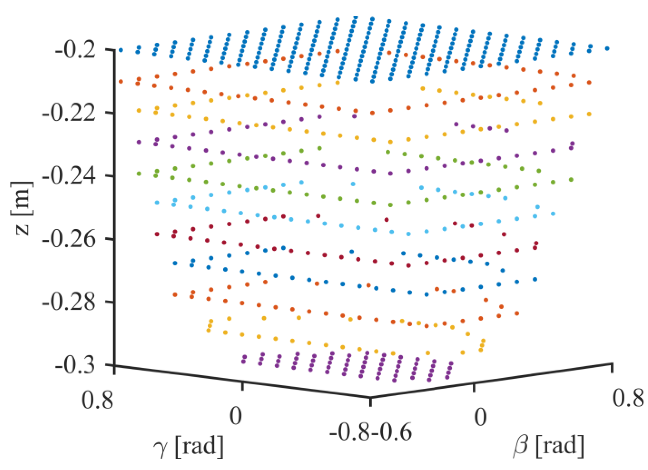
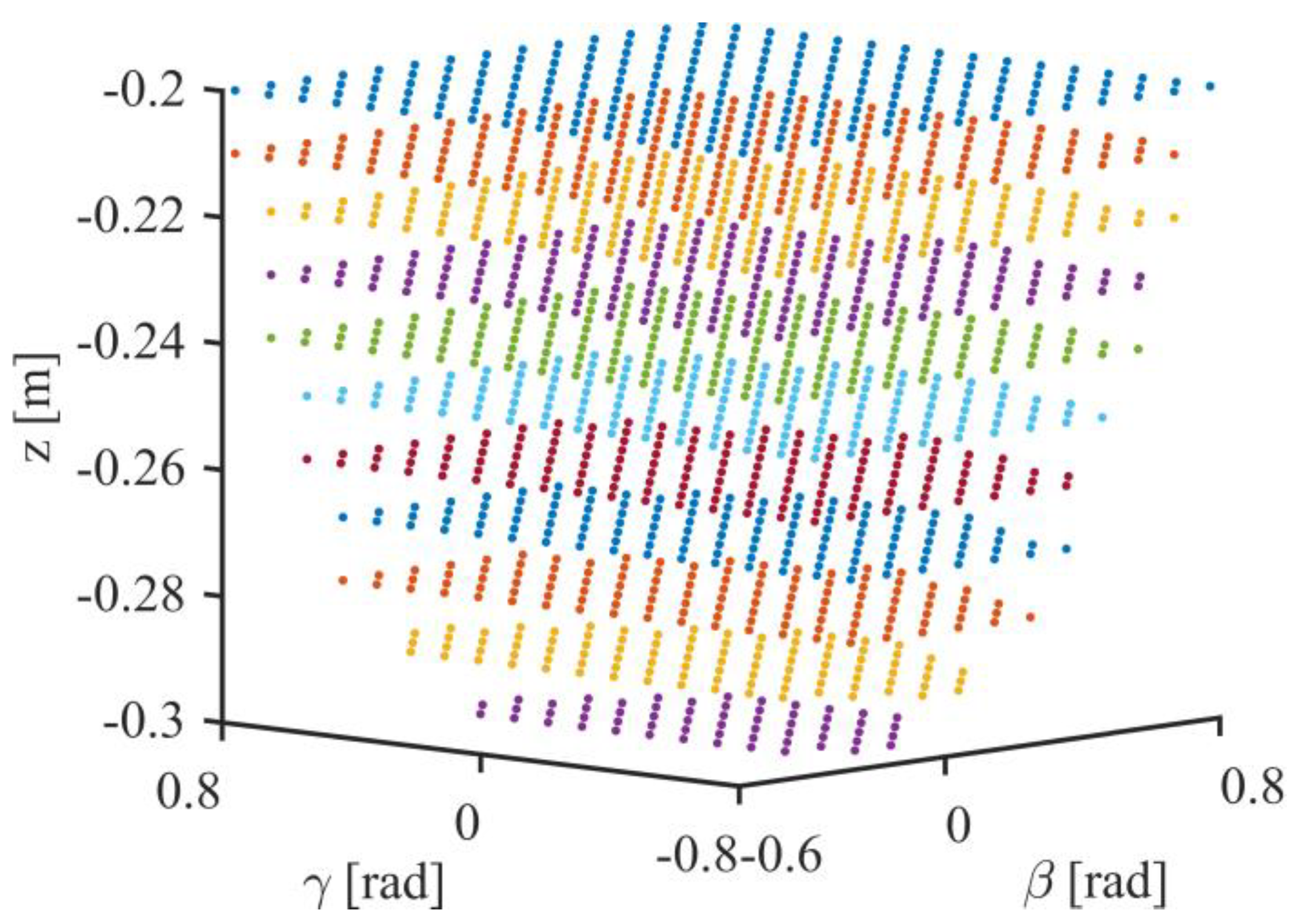
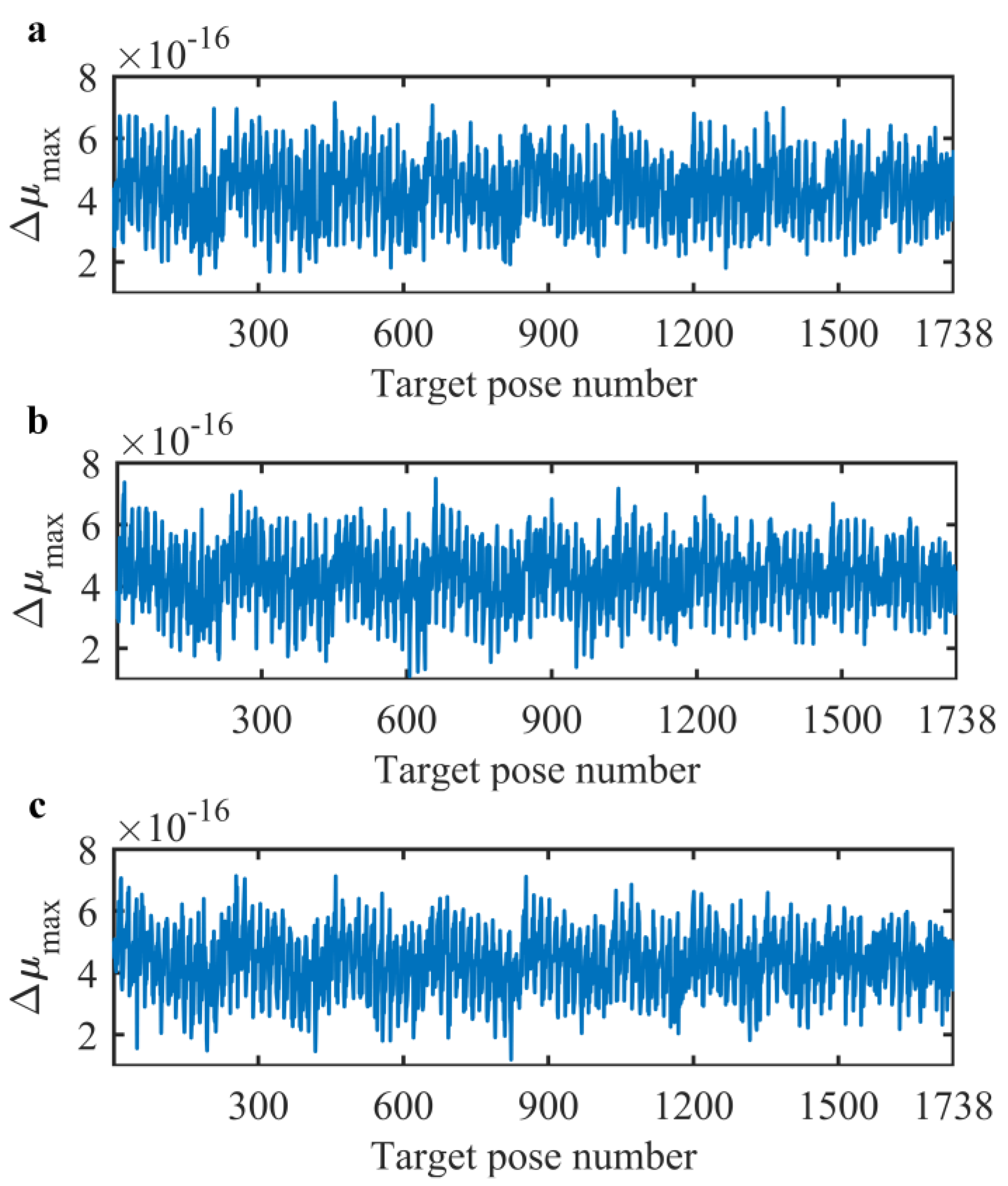
5.2. Simulation Analysis

To validate the correctness of the identified results listed in Table 7, three groups of numerical simulations were conducted using 1738 target poses of the 2UPR-RPU parallel manipulator, as shown in Figure 6. It is assumed that geometric errors are normally distributed with zero means [19,22]. Three groups of standard deviations are listed in

Table 8. Standard deviations of the geometric errors for the numerical simulations.

Symbols	Group 1	Group 2	Group 3	Units
The standard deviations of δi,j	1.6667 × 10−3	3.3333 × 10−5	1.6667 × 10−5	m
The standard deviations of εi,j	1.6667 × 10−3	π/540	π/21,600	rad

. In the simulation, the internal-force-and-deformation-related geometric errors identified in Table 7 were set to 0, and the remaining 30 geometric errors were assigned random values generated by randn function using the standard deviations of δ_i,j and ε_i,j listed in Table 8. Then, according to Scheme I and (45), 1738 $\Delta {\mu }_{\max }$s were calculated for each group. The simulation results are shown in Figure 7. It can be seen that $\Delta {\mu }_{\max }$s of Group 1, Group 2, and Group 3, are all smaller than 10⁻¹⁵. This demonstrates that the internal-force-and-deformation-related geometric errors identified in Section 5.1 are correct.

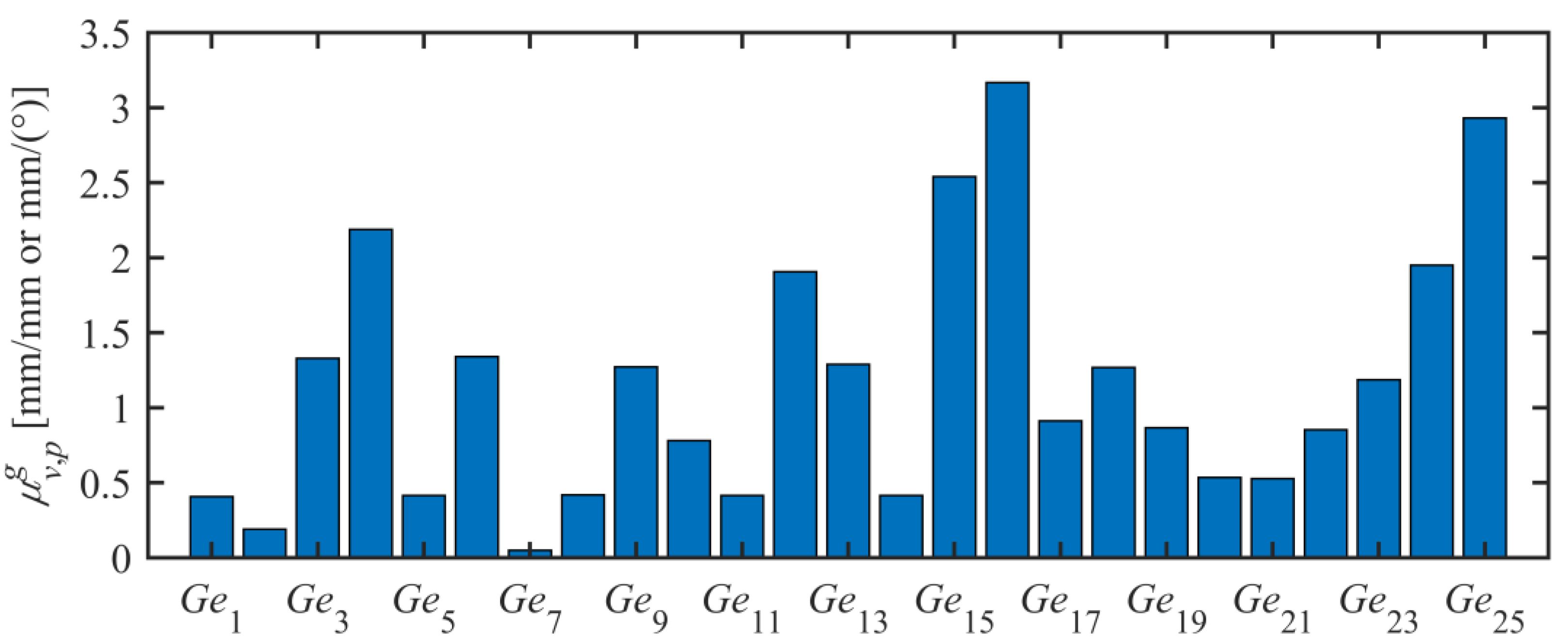
6. Sensitivity Analysis

Sensitivity analysis can help reveal the influence of different internal-force-and-deformation-related geometric errors on the limbs’ comprehensive deformations. Since $\Delta {\mu }^j$ is calculated iteratively in Scheme I, the Monte Carlo method [22] is utilised to conduct sensitivity analysis in this section. Two global sensitivity indices are proposed and the results of sensitivity analysis are verified through simulations.

6.1. Sensitivity Indices

According to (41), $\Delta {\mu }^j$ consists of $\Delta {\mu }_{2,1}^j$, $\Delta {\mu }_{3,2}^j$, and $\Delta {\mu }_{1,3}^j$, which can be written as

$$\Delta {\mu }_{k,i}^j={\left[\begin{array}{cccccc}{\omega }_{k,i,1}^j& {\omega }_{k,i,2}^j& {\omega }_{k,i,3}^j& v_{k,i,1}^j& v_{k,i,2}^j& v_{k,i,3}^j\end{array}\right]}^{\mathrm{T}}$$

(46)

The end-orientation and end-position volumetric deviations between any two limbs are

$$\Delta {\omega }_{k,i}^j=\sqrt{{\left({\omega }_{k,i,1}^j\right)}^2+{\left({\omega }_{k,i,2}^j\right)}^2+{\left({\omega }_{k,i,3}^j\right)}^2}$$

(47)

and

$$\Delta v_{k,i}^j=\sqrt{{\left(v_{k,i,1}^j\right)}^2+{\left(v_{k,i,2}^j\right)}^2+{\left(v_{k,i,3}^j\right)}^2}$$

(48)

Then, the evaluation indices of the average angular and linear comprehensive deformations of the three limbs can be written as

$$\Delta {\omega }_a^j=\frac{\Delta {\omega }_{2,1}^j+\Delta {\omega }_{3,2}^j+\Delta {\omega }_{1,3}^j}{3}$$

(49)

and

$$\Delta v_a^j=\frac{\Delta v_{2,1}^j+\Delta v_{3,2}^j+\Delta v_{1,3}^j}{3}$$

(50)

Under the condition that geometric errors are normally distributed with zero means, the sensitivity indices of the average angular and linear comprehensive deformations with respect to a geometric error can be written as

$${\mu }_{\omega ,p}=\frac{\sigma \left(\Delta {\omega }_{a,p}^j\right)}{\sigma \left(G{e}_p\right)}, p=1, 2, \cdots , 25$$

(51)

and

$${\mu }_{v,p}=\frac{\sigma \left(\Delta v_{a,p}^j\right)}{\sigma \left(G{e}_p\right)}, p=1, 2, \cdots , 25$$

(52)

where $\sigma (\cdot )$ denotes the standard deviation and can be calculated by std function. Ge_ps are the internal-force-and-deformation-related geometric errors of the first and third limbs. Because of the symmetric distribution of the first and second limbs, the internal-force-and-deformation-related geometric errors of the second limb are not considered. Generally, the values of sensitivity indices vary with different target poses of the moving platform. Hence, m target poses should be chosen and the global sensitivity indices can be written as [16]

$${\mu }_{\omega ,p}^g=\frac{{\displaystyle \sum _{i=1}^m{\mu }_{\omega ,p,i}}}{m}+\sigma \left({\mu }_{\omega ,p}\right)$$

(53)

and

$${\mu }_{v,p}^g=\frac{{\displaystyle \sum _{i=1}^m{\mu }_{v,p,i}}}{m}+\sigma \left({\mu }_{v,p}\right)$$

(54)

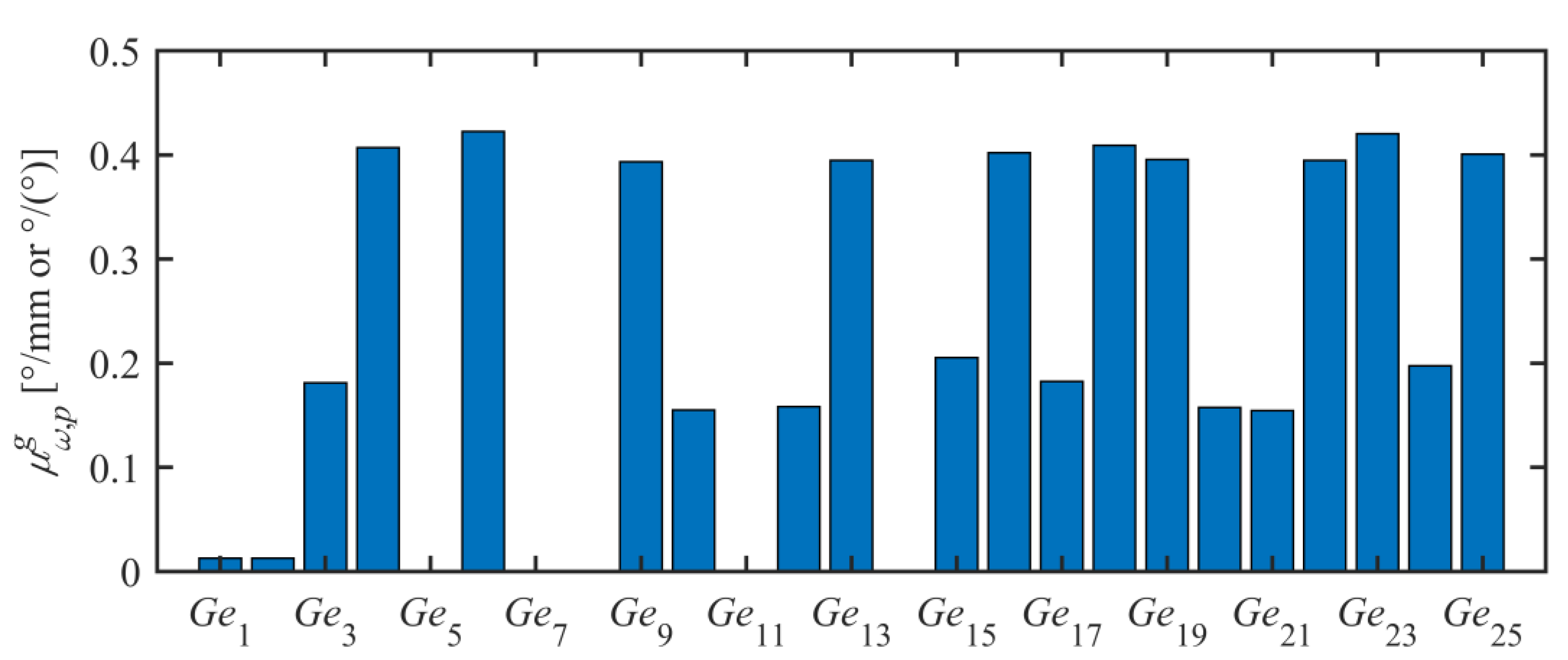
6.2. Sensitivity Analysis

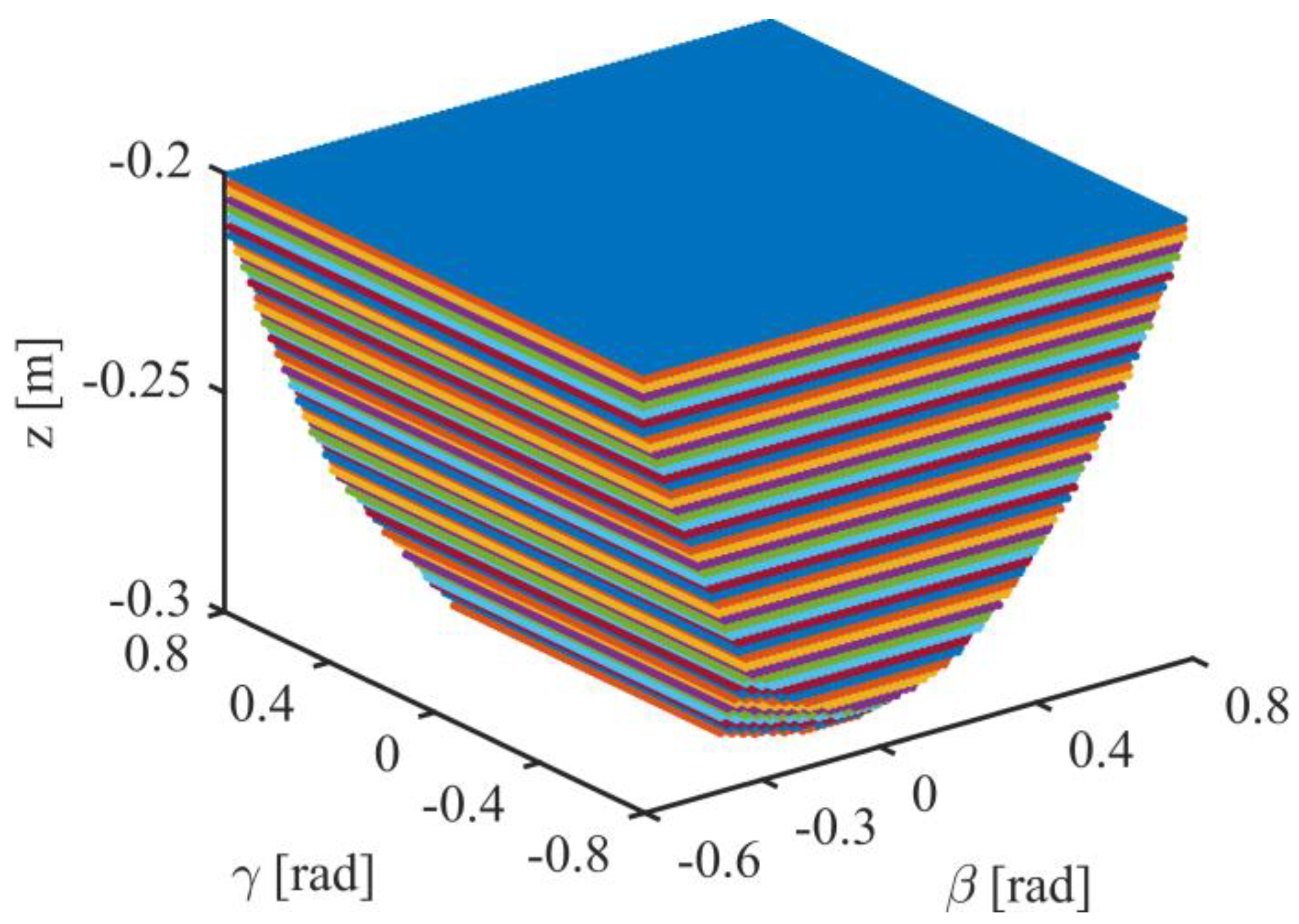
Based on the equations in Section 6.1 and Scheme I, the detailed processes to calculate the two global sensitivity indices with respect to Ge_p are described as follows: (1) Set $\sigma \left(G{e}_p\right)$ to 1 mm (0.001 m) or 1° (π/180 rad) for linear or angular geometric error. And the other 40 internal-force-and-deformation-related geometric errors are set to 0. In addition, the rest 30 linear or angular geometric errors are set to 1 mm or 1°. (2) Assign 1000 random values that obey the normal distribution to Ge_p and calculate 1000 $\Delta {\omega }_{a,p}^j$s and $\Delta v_{a,p}^j$s. (3) Calculate $\sigma \left(\Delta {\omega }_{a,p}^j\right)$, ${\mu }_{\omega ,p}$, $\sigma \left(\Delta v_{a,p}^j\right)$, and ${\mu }_{v,p}$ for a target pose of the moving platform. (4) Repeat the above steps for m target poses and calculate the global sensitivity indices${\mu }_{\omega ,p}^g$ and ${\mu }_{v,p}^g$.

In order to improve the computational efficiency, 158 of the 1738 target poses shown in Figure 6 were selected uniformly to perform the above steps for each Ge_p. The global sensitivity indices of the average angular and linear comprehensive deformations with respect to Ge_ps are shown in Figure 8 and Figure 9, respectively. It can be seen that the values of ${\mu }_{\omega ,p}^g$ with respect to Ge₅(${\delta }_{1,1}^y$), Ge₇(${\epsilon }_{1,1}^z$), Ge₈(${\delta }_{1,2}^z$), Ge₁₁(${\delta }_{1,3}^x$), and Ge₁₄(${\delta }_{1,4}^y$), are zero. This indicates that the corresponding geometric errors have no effects on the average angular comprehensive deformation. It is worth mentioning that ${\delta }_{2,1}^y$, ${\epsilon }_{2,1}^z$, ${\delta }_{2,2}^z$, ${\delta }_{2,3}^x$, and ${\delta }_{2,4}^y$, have also no effects on the average angular comprehensive deformation due to the symmetric distribution of the first and second limbs. Comparing Figure 8 with Figure 9, it can also be found that the value of ${\mu }_{v,p}^g$ is larger than that of ${\mu }_{\omega ,p}^g$ for each Ge_p. This demonstrates that the internal-force-and-deformation-related geometric errors have greater effects on the average linear comprehensive deformation. Thus, the distribution of the global sensitivity index ${\mu }_{v,p}^g$ is more useful for accuracy synthesis. According to Figure 9, Ge_ps can be sorted in descending order as follows: Ge₁₆(${\epsilon }_{1,4}^z$), Ge₂₅(${\epsilon }_{3,4}^z$), Ge₁₅(${\epsilon }_{1,4}^x$), Ge₄(${\epsilon }_{1,0}^z$), Ge₂₄(${\epsilon }_{3,4}^x$), Ge₁₂(${\epsilon }_{1,3}^y$), Ge₆(${\epsilon }_{1,1}^x$), Ge₃(${\epsilon }_{1,0}^y$), Ge₁₃(${\epsilon }_{1,3}^z$), Ge₉(${\epsilon }_{1,2}^x$), Ge₁₈(${\epsilon }_{3,0}^z$), Ge₂₃(${\epsilon }_{3,3}^x$), Ge₁₇(${\epsilon }_{3,0}^y$), Ge₁₉(${\epsilon }_{3,1}^x$), Ge₂₂(${\epsilon }_{3,2}^z$), Ge₁₀(${\epsilon }_{1,2}^y$), Ge₂₀(${\epsilon }_{3,1}^y$), Ge₂₁(${\epsilon }_{3,2}^y$), Ge₈(${\delta }_{1,2}^z$), Ge₁₄(${\delta }_{1,4}^y$), Ge₅(${\delta }_{1,1}^y$), Ge₁₁(${\delta }_{1,3}^x$), Ge₁(${\delta }_{1,0}^y$), Ge₂(${\delta }_{1,0}^z$), and Ge₇(${\epsilon }_{1,1}^z$). In order to lower the cost of fabrication and assembly, the allowable range of geometric errors should be larger and larger from Ge₁₆ to Ge₇.

6.3. Verification

6.3.1. Average Angular Comprehensive Deformation

As shown in

Table 9. Sensitivity analysis results of the average angular comprehensive deformation.

Group Number	Ge5$, G{e}_7, G{e}_8, G{e}_{11}, G{e}_{14}, {\delta }_{2,1}^y$$,{\epsilon }_{2,1}^z$$, {\delta }_{2,2}^z$$, {\delta }_{2,3}^x$$, {\delta }_{2,4}^y$ [mm or °]	Other Geometric Errors [mm or °]	$\mathrm{The} \mathrm{Maximum} \mathrm{Value} \mathrm{of} \Delta {\omega }_a^j$ [°]	$\mathrm{The} \mathrm{Average} \mathrm{Value} \mathrm{of} \Delta {\omega }_a^j$ [°]
Group 1	0.1	0.1	0.1430	0.0961
Group 2	0.01	0.1	0.1430	0.0961
Group 3	0.001	0.1	0.1430	0.0961

, three groups of specified values for geometric errors are given. For each group, 1738 $\Delta {\omega }_a^j$s were calculated according to Scheme I and using the target poses shown in Figure 6. The maximum and average values of $\Delta {\omega }_a^j$ are listed in Table 9. It can be seen that both the maximum and average values of $\Delta {\omega }_a^j$ do not change from Group 1 to Group 3. This indicates that Ge₅, Ge₇, Ge₈, Ge₁₁, Ge₁₄, ${\delta }_{2,1}^y$, ${\epsilon }_{2,1}^z$, ${\delta }_{2,2}^z$, ${\delta }_{2,3}^x$, and ${\delta }_{2,4}^y$, have no effects on the average angular comprehensive deformation.

6.3.2. Average Linear Comprehensive Deformation

As shown in

Table 10. Specified geometric errors for verification.

i	j	${\delta }_{i,j}^x$ [mm]	${\delta }_{i,j}^y$ [mm]	${\delta }_{i,j}^z$ [mm]	${\epsilon }_{i,j}^x$ [°]	${\epsilon }_{i,j}^y$ [°]	${\epsilon }_{i,j}^z$ [°]
1, 2	0	0.1	0.0177	0.0381	–	0.0054	0.0033
1, 2	1	0.1	0.0174	0.1	0.0053	–	1
1, 2	2	–	0.1	0.0173	0.0056	0.0092	0.1
1, 2	3	0.0174	0.1	–	–	0.0037	0.0056
1, 2	4	0.1	0.0174	0.1	0.0028	–	0.0022
3	0	0.1	0.1	0.1	–	0.0079	0.0057
3	1	–	0.1	0.1	0.0083	0.0135	0.1
3	2	0.1	0.1	–	–	0.0137	0.0084
3	3	0.1	0.1	0.1	0.0061	–	–
3	4	0.1	0.1	0.1	0.0037	–	0.0024

, Ge₇(${\epsilon }_{1,1}^z$), which has the smallest effect on the average linear comprehensive deformation, is set to 1°. Then, the other Ge_ps are set to ${\mu }_{v,7}^g/{\mu }_{v,p}^g$ mm or °. It is worth mentioning that the corresponding internal-force-and-deformation-related geometric errors of the second limb are assigned the same values as the first limb due to the symmetric distribution of the two UPR limbs. The remaining 30 geometric errors are set to 0.1 mm or °. According to Scheme I and using the target poses shown in Figure 6, 1738$\Delta {\omega }_a^j$s and $\Delta v_a^j$s were calculated. For comparison, the internal-force-and-deformation-related linear and angular geometric errors are set to their average values, 0.0209 mm and 0.0743 °, respectively, while the values of the remaining 30 geometric errors are unchanged. After recalculation, the maximum and average values of $\Delta {\omega }_a^j$ and $\Delta v_a^j$ are listed in

Table 11. Sensitivity analysis results of the average linear comprehensive deformation.

Group Number	$\mathbf{The} \mathbf{Maximum} \mathbf{Value} \mathbf{of} \mathit{\Delta }{\mathit{\omega }}_{\mathit{a}}^{\mathit{j}}$ [°]	$\mathbf{The} \mathbf{Average} \mathbf{Value} \mathbf{of} \mathit{\Delta }{\mathit{\omega }}_{\mathit{a}}^{\mathit{j}}$ [°]	$\mathbf{The} \mathbf{Maximum} \mathbf{Value} \mathbf{of} \mathit{\Delta }{\mathit{v}}_{\mathit{a}}^{\mathit{j}}$ [mm]	$\mathbf{The} \mathbf{Average} \mathbf{Value} \mathbf{of} \mathit{\Delta }{\mathit{v}}_{\mathit{a}}^{\mathit{j}}$ [mm]
Group 1	0.0165	0.0118	0.0696	0.0390
Group 2	0.1061	0.0714	0.8374	0.3581

. It can be seen that both the maximum and average values of $\Delta v_a^j$ are larger than that of $\Delta {\omega }_a^j$ for each group. This indicates that the internal-force-and-deformation-related geometric errors have greater effects on the average linear comprehensive deformation. It can also be found that from Group 2 to Group 1, the maximum and average values of $\Delta {\omega }_a^j$ and $\Delta v_a^j$ decreased by 84%, 83%, 91%, and 89%, respectively. This demonstrates that at the same cost, restricting the values of geometric errors according to the sensitivity analysis results of the average linear comprehensive deformation can dramatically decrease the average angular and linear comprehensive deformations. Furthermore, it indirectly verifies the sensitivity analysis results of the average linear comprehensive deformation.

7. Conclusions

This paper deals with error modelling and sensitivity analysis of geometric errors that cause internal forces and deformations in the 2UPR-RPU over-constrained parallel manipulator. Conclusions are drawn as follows:

(1) The nominal inverse kinematics and actual forward kinematics of the over-constrained parallel manipulator are analysed according to the vector theory and the local product of the exponential formula. On this basis, an iterative model is established to indirectly evaluate the limbs’ comprehensive deformations caused by geometric errors.

(2) Based on the iterative evaluation model, the maximum Euclidean norm of the end-pose deviations of limbs is defined as an evaluation index of the maximum comprehensive deformation of a limb. Programming with MATLAB, 41 internal-force-and-deformation-related geometric errors are identified. Among the 41 geometric errors, the number of angular geometric errors is greater than that of linear geometric errors; the geometric errors of the first UPR limb are the same as those of the second UPR limb; the geometric errors of the RPU limb are all angular geometric errors. The correctness of the identification results is verified through simulations under the condition that geometric errors are normally distributed with zero means.

(3) The global sensitivity indices of the average angular and linear comprehensive deformations with respect to internal-force-and-deformation-related geometric errors are proposed and calculated based on the Monte Carlo method. The results of sensitivity analysis demonstrate that ${\delta }_{1,1}^y$, ${\epsilon }_{1,1}^z$, ${\delta }_{1,2}^z$, ${\delta }_{1,3}^x$, ${\delta }_{1,4}^y$, ${\delta }_{2,1}^y$, ${\epsilon }_{2,1}^z$, ${\delta }_{2,2}^z$, ${\delta }_{2,3}^x$, and ${\delta }_{2,4}^y$, have no effects on the average angular comprehensive deformation. Furthermore, the internal-force-and-deformation-related geometric errors have greater effects on the average linear comprehensive deformation. Therefore, the distribution of the global sensitivity index of the average linear comprehensive deformation with respect to geometric errors is more meaningful for accuracy synthesis. Finally, the results of sensitivity analysis are verified through simulations.

Based on the work presented in this paper, we will establish a model for accuracy synthesis and determine the tolerances of the fabrication and assembly of the manipulator in the future.

References

1. Tang, T.F.; Fang, H.L.; Zhang, J. Hierarchical design, laboratory prototype fabrication and machining tests of a novel 5-axis hybrid serial-parallel kinematic machine tool. Robot. Comput.-Integr. Manuf. 2020, 64, 101944. [Google Scholar] [CrossRef]
2. Xie, F.G.; Liu, X.J.; Li, T.M. Type synthesis and typical application of 1T2R-type parallel robotic mechanisms. Math. Probl. Eng. 2013, 2013, 206181. [Google Scholar] [CrossRef] [Green Version]
3. Li, Q.C.; Hervé, J.M. Type synthesis of 3-DOF RPR-equivalent parallel mechanisms. IEEE Trans. Robot. 2014, 30, 1333–1343. [Google Scholar] [CrossRef]
4. Li, Q.; Xu, L.; Chen, Q.; Ye, W. New family of RPR-equivalent parallel mechanisms: Design and application. Chin. J. Mech. Eng. 2017, 30, 217–221. [Google Scholar] [CrossRef]
5. Huang, T.; Dong, C.; Liu, H.; Sun, T.; Chetwynd, D.G. A simple and visually orientated approach for type synthesis of overconstrained 1T2R parallel mechanisms. Robotica 2019, 37, 1161–1173. [Google Scholar] [CrossRef] [Green Version]
6. Tang, T.; Fang, H.; Luo, H.; Song, Y.; Zhang, J. Type synthesis, unified kinematic analysis and prototype validation of a family of Exechon inspired parallel mechanisms for 5-axis hybrid kinematic machine tools. Robot. Comput.-Integr. Manuf. 2021, 72, 102181. [Google Scholar] [CrossRef]
7. Zhao, Y.; Xu, Y.; Yao, J.; Jin, L. A force analysis method for overconstrained parallel mechanisms. China Mech. Eng. 2014, 25, 711–717. [Google Scholar] [CrossRef]
8. Chai, X.X.; Xiang, J.N.; Li, Q.C. Singularity analysis of a 2-UPR-RPU parallel mechanism. J. Mech. Eng. Chin. Ed. 2015, 51, 144–151. [Google Scholar] [CrossRef] [Green Version]
9. Jiang, Y.; Li, T.; Wang, L.; Chen, F. Kinematic error modeling and identification of the over-constrained parallel kinematic machine. Robot. Comput.-Integr. Manuf. 2018, 49, 105–119. [Google Scholar] [CrossRef]
10. He, L.; Li, Q.; Zhu, X.; Wu, C.-Y. Kinematic calibration of a three degrees-of-freedom parallel manipulator with a laser tracker. J. Dyn. Syst. Meas. Control 2019, 141, 031009. [Google Scholar] [CrossRef]
11. Song, Y.M.; Zhai, Y.P.; Sun, T. Interval analysis based accuracy design of a 3-DOF rotational parallel mechanism. J. Beijing Univ. Technol. 2015, 41, 1620–1626,1755. [Google Scholar]
12. Ni, Y.; Zhang, B.; Sun, Y.; Zhang, Y. Accuracy analysis and design of A3 parallel spindle head. Chin. J. Mech. Eng. 2016, 29, 239–249. [Google Scholar] [CrossRef]
13. Zhang, J.; Chi, C.C.; Jiang, S.J. Accuracy design of 2UPR-RPS parallel mechanism. Trans. Chin. Soc. Agric. Eng. 2021, 52, 411–420. [Google Scholar] [CrossRef]
14. Huang, T.; Whitehouse, D.J.; Chetwynd, D.G. A unified error model for tolerance design, assembly and error compensation of 3-DOF parallel kinematic machines with parallelogram struts. CIRP Ann. 2002, 51, 297–301. [Google Scholar] [CrossRef]
15. Zhang, J.T.; Lian, B.B.; Song, Y.M. Geometric error analysis of an over-constrained parallel tracking mechanism using the screw theory. Chin. J. Aeronaut. 2019, 32, 1541–1554. [Google Scholar] [CrossRef]
16. Luo, X.; Xie, F.; Liu, X.-J.; Li, J. Error modeling and sensitivity analysis of a novel 5-degree-of-freedom parallel kinematic machine tool. Proc. Inst. Mech. Eng. Part B J. Eng. Manuf. 2019, 233, 1637–1652. [Google Scholar] [CrossRef]
17. Wang, W.; Yun, C. Orthogonal experimental design to synthesize the accuracy of robotic mechanism. J. Mech. Eng. Chin. Ed. 2009, 45, 18–24. [Google Scholar] [CrossRef]
18. Yao, R.; Zhu, W.B.; Huang, P. Accuracy analysis of stewart platform based on interval analysis method. Chin. J. Mech. Eng. 2013, 26, 29–34. [Google Scholar] [CrossRef]
19. Wu, M.; Yue, X.; Chen, W.; Nie, Q.; Zhang, Y. Accuracy analysis and synthesis of asymmetric parallel mechanism based on Sobol-QMC. Proc. Inst. Mech. Eng. Part C J. Mech. Eng. Sci. 2020, 234, 4200–4214. [Google Scholar] [CrossRef]
20. Li, X.Y.; Chen, W.Y.; Han, X.G. Accuracy analysis and synthesis of 3-RPS parallel machine based on orthogonal design. J. Beijing Univ. Aeronaut. Astronaut. 2011, 37, 979–984. [Google Scholar] [CrossRef]
21. Tai-Ke, Y.; Xi, Z.; Feng, Z.; Li-Min, Z.; Yong, W. Accuracy synthesis of a 3-RPS parallel robot based on manufacturing costs. In Proceedings of the 31st Chinese Control Conference, Hefei, China, 25–27 July 2012; pp. 5168–5172. [Google Scholar]
22. Liu, H.T.; Pan, Q.; Yin, F.W.; Dong, C.L. Accuracy synthesis of the TriMule hybrid robot. J. Tianjin Univ. Sci. Technol. 2019, 52, 1245–1254. [Google Scholar]
23. Tang, T.; Luo, H.; Song, Y.; Fang, H.; Zhang, J. Chebyshev inclusion function based interval kinetostatic modeling and parameter sensitivity analysis for Exechon-like parallel kinematic machines with parameter uncertainties. Mech. Mach. Theory 2021, 157, 104209. [Google Scholar] [CrossRef]
24. Yu, D.; Zhao, Q.; Guo, J.; Chen, F.; Hong, J. Accuracy analysis of spatial overconstrained extendible support structures considering geometric errors, joint clearances and link flexibility. Aerosp. Sci. Technol. 2021, 119, 107098. [Google Scholar] [CrossRef]
25. Chen, G.; Kong, L.; Li, Q.; Wang, H.; Lin, Z. Complete, minimal and continuous error models for the kinematic calibration of parallel manipulators based on POE formula. Mech. Mach. Theory 2018, 121, 844–856. [Google Scholar] [CrossRef]
26. Kong, L.; Chen, G.; Wang, H.; Huang, G.; Zhang, D. Kinematic calibration of a 3-PRRU parallel manipulator based on the complete, minimal and continuous error model. Robot. Comput.-Integr. Manuf. 2021, 71, 102158. [Google Scholar] [CrossRef]
27. Sun, T.; Song, Y.; Li, Y.; Xu, L. Separation of comprehensive geometrical errors of a 3-DOF parallel manipulator based on Jacobian matrix and its sensitivity analysis with Monte-Carlo method. Chin. J. Mech. Eng. 2011, 24, 406–413. [Google Scholar] [CrossRef]
28. Chen, Y.; Xie, F.; Liu, X.; Zhou, Y. Error modeling and sensitivity analysis of a parallel robot with SCARA (selective compliance assembly robot arm) motions. Chin. J. Mech. Eng. 2014, 27, 693–702. [Google Scholar] [CrossRef]
29. Ma, J.G. Kinematics Analysis and Parameter Optimization of 2UPR-RPU Parallel Mechanism. Master’s Thesis, Zhejiang Sci-Tech University, Hangzhou, China, 2014. [Google Scholar] [CrossRef]
30. Selig, J.M. Geometric Fundamentals of Robotics; Springer: New York, NY, USA, 2005. [Google Scholar] [CrossRef]
31. Dai, J.S. Screw Algebra and Lie Groups and Lie Algebras; Higher Education Press: Beijing, China, 2014. [Google Scholar]
Figure 1. Schematic diagram of the 2UPR-RPU parallel mechanism.
Machines 10 00990 g001
Figure 2. 2UPR-RPU parallel manipulator and its local coordinate systems.
Machines 10 00990 g002
Figure 3. Scheme I: Evaluation of the limbs’ comprehensive deformations caused by geometric errors of the 2UPR-RPU over-constrained manipulator.
Machines 10 00990 g003
Figure 4. Reachable workspace of the 2UPR-RPU parallel manipulator.
Machines 10 00990 g004
Figure 5. 692 target poses of the 2UPR-RPU parallel manipulator.
Machines 10 00990 g005
Figure 6. 1738 target poses of the 2UPR-RPU parallel manipulator.
Machines 10 00990 g006
Figure 7. Simulation results using the standard deviations listed in Table 8. (a) Group 1; (b) Group 2; (c) Group 3.
Machines 10 00990 g007
Figure 8. Global sensitivity of the average angular comprehensive deformation with respect to Geps.
Machines 10 00990 g008
Figure 9. Global sensitivity of the average linear comprehensive deformation with respect to Geps.
Machines 10 00990 g009