1. Introduction
Grinding is a widespread but essential process in manufacturing products. It is widely used in aerospace, automobile manufacturing, rail transit and other industries [
1]. Traditionally, grinding is done by manual operation or multi-axis CNC machine tools. The former is time-consuming and labor-intensive, while the latter is limited by operating space. Recently, robotic belt grinding has become an alternative due to its low cost, efficiency and large operating space [
2]. For small workpiece, the robot generally uses appropriate contact force to ensure the stability of the workpiece [
3]. The robot holds the workpiece to complete the grinding operation and uses its dexterity to move to the best inspection position on the surface of the workpiece [
4]. Multiple sampling points are planned according to the curvature of the workpiece surface, and the robot moves to each sampling point in turn to complete the surface image sampling.
As an important indicator of the quality of machined surfaces, surface roughness has a significant impact on product life and reliability [
5]. The traditional probe-based measurement method [
6,
7,
8,
9] uses a probe that slides over the surface of the workpiece for measurement. This method has been proven to be highly reliable and highly accurate. However, it has several limitations, such as long measurement times, high environmental requirements and complex steps.
With the development of optical technology, a variety of noncontact measurement methods has been developed to address the limitations of the contact measurement method. For example, optical microscopy, confocal laser scanning microscopy and white light interferometry are used to measure surface roughness, but these methods are mainly used in laboratories, because their high cost and complicated operation are not suitable for real industrial production. Currently, the most popular noncontact measurement method is based on machine vision for roughness measurements of the machined workpiece surface [
10,
11,
12,
13,
14,
15]; this is widely used because of its advantages, which include unrestricted size of the measured object, low cost, high speed, and easy factory automation deployment.
Usually, vision-based measurement methods can be divided into four stages: image acquisition, image processing, feature extraction and prediction strategy [
16]. Most vision-based methods for surface roughness assessments rely on feature extraction. Suganandha et al. [
17] used a single-point laser to irradiate the surface of an object and analyzed the gray-level covariance matrix (GLCM) features of the scatter pattern, such as contrast, correlation, energy, entropy homogeneity and maximum probability, in order to investigate the correlation between 3D surface roughness and scatter images. Shanta et al. [
18] obtained roughness measures by using a singular value decomposition method to analyze contrast, as well as light and dark pixels of binarized scatter patterns. Samie et al. [
19] proposed a method to transform the image of a surface into an unweighted and undirected network graph. The graph-theoretic invariants and Fiedler number were estimated for use as discriminative factors for the surface roughness of the workpiece, avoiding the filtering and segmentation of complex images. Liu et al. [
20] proposed an improved method based on microscopic vision to detect the surface roughness of R surfaces in valves. The method analyzed the surface morphology images of R surfaces by the gray-level covariance matrix (GLCM) method and used a support vector machine (SVM) model to describe the relationship between GLCM features and the actual surface roughness. Huaian et al. [
21] used a specific of color light source to illuminate the surface and measured the surface roughness of the object based on the color distribution statistical matrix for features such as texture in the image.
Vision-based surface roughness assessment methods have been proven to be reliable and accurate, but there are still some limitations, especially in the feature extraction process. Visual assessment methods that rely on feature extraction are difficult to reapply to different datasets. Feature extraction is a highly intensive process that requires a high degree of computation and expert decision making in selecting the appropriate surface features. As a result, the process can lead to long processing times, which are not conducive to the rapid diffusion of the technique.
Some researchers had accomplished roughness measurement by using intelligent algorithms for the self-learning of image features. For example, Du-Ming [
22] used the two-dimensional Fourier transform to extract quantitative measures of surface roughness in the spatial frequency domain. The roughness features were used as input to build an artificial neural network to determine the surface roughness. Gürcan [
23] converted the surface image into a binary image as input data. The log-sigmoid function was chosen as the transfer function and the neural network model was trained using the scaled conjugate gradient algorithm. Kaixuan et al. [
24] proposed a roughness classification method. The method expanded and preprocessed the images, and then trained an AlexNet-based surface roughness classification model for milled samples.
Jamal et al. [
25] proposed that a convolutional neural network (CNN) is used as a regressor in order to obtain steel surface roughness, and that a CNN based on spatial pooling pyramid is applied for roughness classification. Achmad et al. [
26] proposed a deep learning model containing convolutional layer, ReLU, pooling layer and two FC layers to automatically learn image features using a gradient descent method to optimize hyperparameters in the model.
GAN is an emerging self-supervised learning technique that provides a method to learn deep representations without the use of extensively labeled training data [
27,
28].
In this paper, we design a surface roughness prediction model based on GAN + BP neural network. Firstly, we consider the difference in surface images with different curvatures and use the images and curvatures as training samples. Then, the GAN network performs model training in such a way that the generative network and the discriminative network play with each other to automatically learn the features in the images, omitting the feature extraction step. Finally, the BP neural network represents the correlation between the GAN discriminant value and the roughness (Ra).
2. Generative Adversarial Network
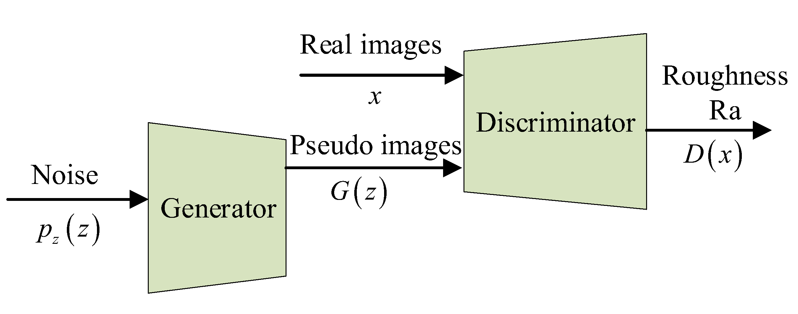
A GAN consists of two parts: the generative and discriminative networks, which use an adversarial game between generators and discriminators to achieve self-supervised learning. The main difference from the traditional network model is that the data training process contains both consistent and adversarial data. The generators and discriminators each optimize in different directions and form a competitive relationship with each other, but they also depend on each other to form a unified whole. In the adversarial training mode, the generator no longer learns directly from the training dataset, but learns iteratively in an indirect way through the optimization directions output by the discriminator, generating pseudosamples to mix the spurious with the genuine. A GAN computes faster and has greater expansion flexibility than a traditional network. In this paper, we propose using a GAN to discriminate the roughness of the surface of workpieces using the structure shown in
Figure 1.
represented a prior on input noise variables,
was generator of GAN, and
represented the probability that x comes from real images. GAN’s goal is training
to maximize the probability of assigning the correct label to both training real samples and pseudosamples from
, at the same time training
to minimize
. In other words, the loss function of GAN is as follows:
The disadvantages of GAN:
(1) GAN training is unstable, and the training degree of generator and discriminator should be carefully balanced.
(2) When the generator learns that some features of the real data successfully deceive the discriminator, it will not update. As a result, the generated samples lack diversity, and a collapse mode occurs in GAN.
(3) When the overlap between the real and generated distributions is negligible, the JS divergence between the real and generated distributions is minimized to a constant log2. When the discriminator is optimal, the loss of the minimized generator is also closer to log2, and G is no longer updated, resulting in the disappearance of the generator gradient.
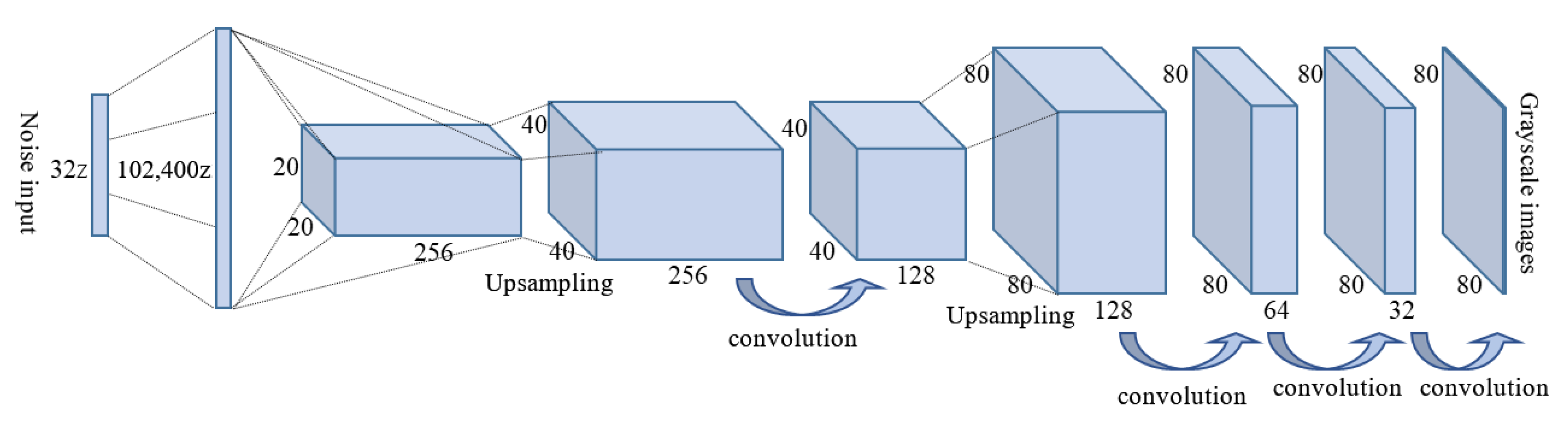
In order to overcome the above shortcomings, the generator and discriminator network structures of the original GAN network are redesigned. In this paper, a deep convolutional neural network is used as the network structure of the generator and discriminator:
The structure of the generative network is shown in
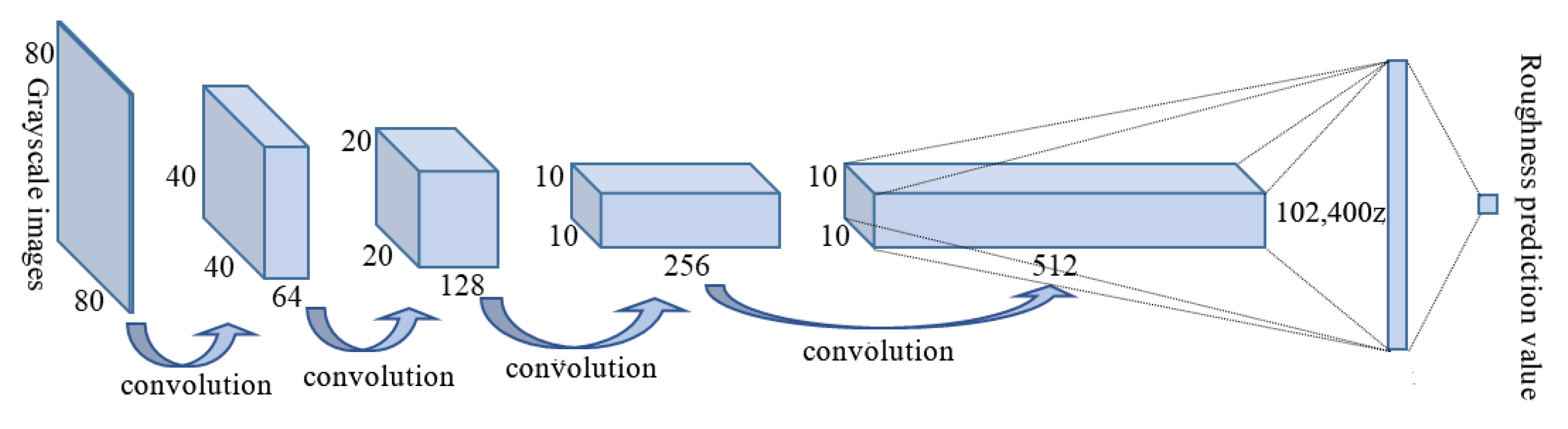
Figure 2, and the corresponding discriminator network structure is shown in
Figure 3.
From Equation (1), it can be seen that the objective of the discriminator is to obtain the maximum value of . Then, it is necessary to maximize , which means maximizing the probability that real samples and generated samples will be assigned the correct label. At the same time, the generator is trained to minimize , which means minimizing the difference between the generated samples and the true samples.
Therefore, the value function of GAN can be decomposed into two optimization problems:
(1) Fix the generator
, train the discriminator
, so that it can maximize the correct determination of whether the sample is from the real sample or from the sample generated by
. The objective function of
is,
Finding the derivative of Equation (2) with respect to
, such that its derivative 0 gives,
Rewriting Equation (3), the optimal discriminator is obtained as follows:
(2) Fix the discriminator
and train the generator
, such that
minimizes the difference between the generated samples and the real samples. The objective function of
is given by,
Substituting Equation (4) into Equations (2) and (5), we obtain,
Introducing two important similarity metrics KL divergence (Kullback–Leibler divergence) and JS divergence (Jensen–Shannon divergence), Equation (6) is rewritten as,
From Equation (7), it can be seen that fixing the discriminator, the goal of training the generator is to have a JS dispersion of 0 between and , i.e., . At this point, the discriminator . Thus, the equilibrium between generator and discriminator is realized by reciprocally training the GAN.
3. Measurement of Surface Roughness of Workpieces
In this method, a neural network is used to discriminate the surface roughness of a grinded workpiece. A small number of data images are used to train a generative adversarial network (GAN) to generate the required large dataset for training the discriminative network, which outputs the surface roughness measurements of the workpiece.
3.1. Image Acquisition and Data Preprocessing Methods Subsection
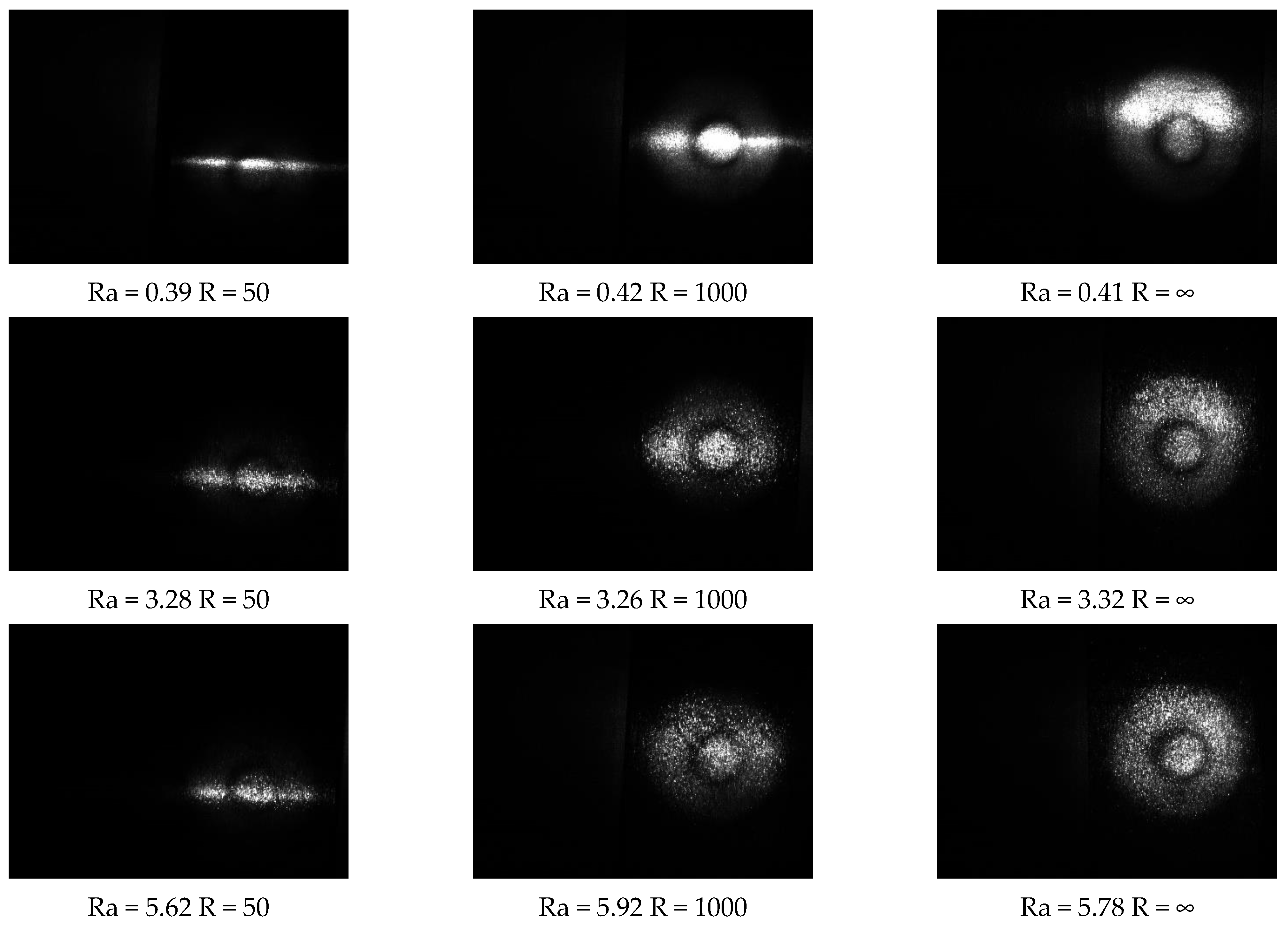
The radius of the curvature and roughness of the workpiece surface directly determine the refractive index of light, a factor which affects the imaging effect of the workpiece surface.
Therefore, 72 images of workpieces with different curvature radii and roughness were collected in this study. The 12 images with the roughest and smoothest surfaces were selected as the original training dataset for the GAN generator, with 6 smooth and 6 rough images, as shown in
Figure 4. However, the amount of data in the original dataset of 12 images was too small to be used directly for training the GAN discriminator, which would lead to severe overfitting of the discriminator. Therefore, the original images were first rotated and panned to generate a sufficient number of derived images (32,000 images were generated in the experiment).
3.2. GAN-Based Surface Roughness Discrimination Method
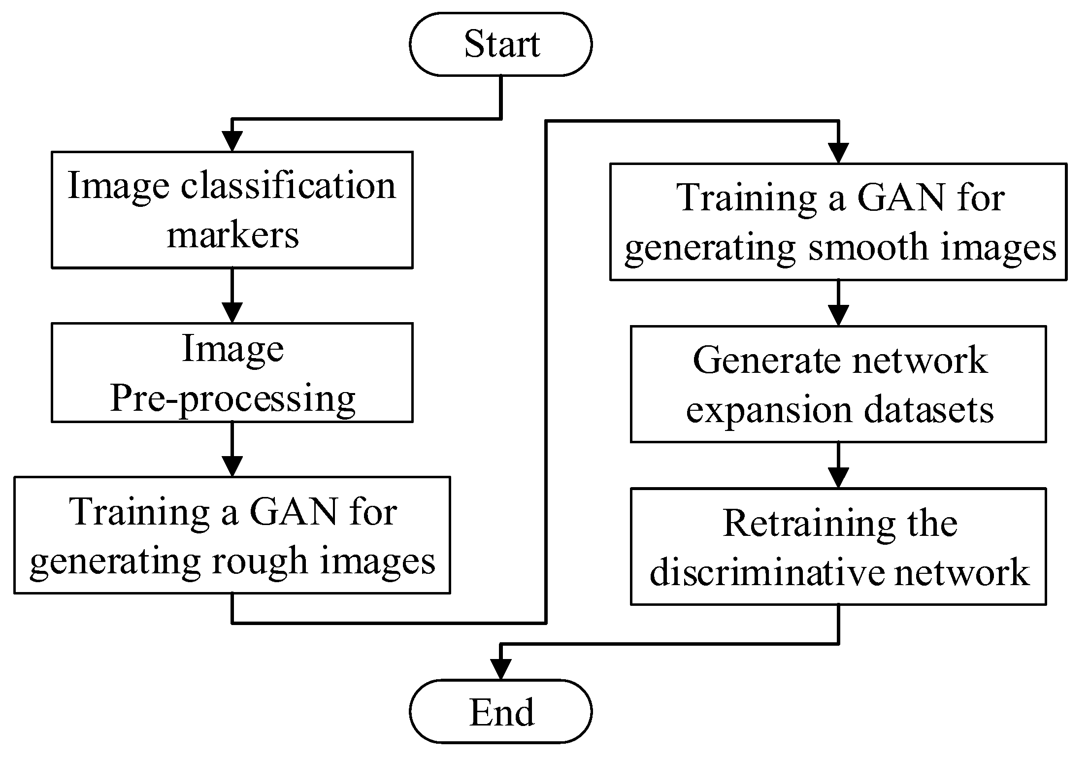
The generative network attempts to create images that the discriminant network cannot distinguish from real images during the training process, while the discriminant network is equivalent to a binary classification network to distinguish between the real training images and the images created by the generator. In this way, the model parameters are continuously optimized by the adversarial training between the two networks. Over multiple iterations, the images created by the generative network become closer to the real images, and the discriminant network increasingly understands the meaning of the roughness represented by the images, and finally gives the roughness value.
The process of training the GAN is shown in
Figure 5.
Step 1: The original datasets (surface roughness images) are classified in a binary fashion and labeled as “smooth” and “rough” according to a certain threshold.
Step 2: Real surface roughness images marked by the classification in step 1 are rotated and panned to expand datasets.
Step 3: The GAN is trained using the “rough” category data in the dataset in Step 2.
Step 4: The GAN is trained using the “smooth” category data in the dataset in Step 2.
Step 5: The image data is generated from the generation network trained in steps 3 and 4 to complete the data set expansion.
Step 6: The discriminative network is retrained for the expanded smooth and rough datasets generated by the generative network in step 5 to obtain the final roughness recognition network model.
3.3. Training Results
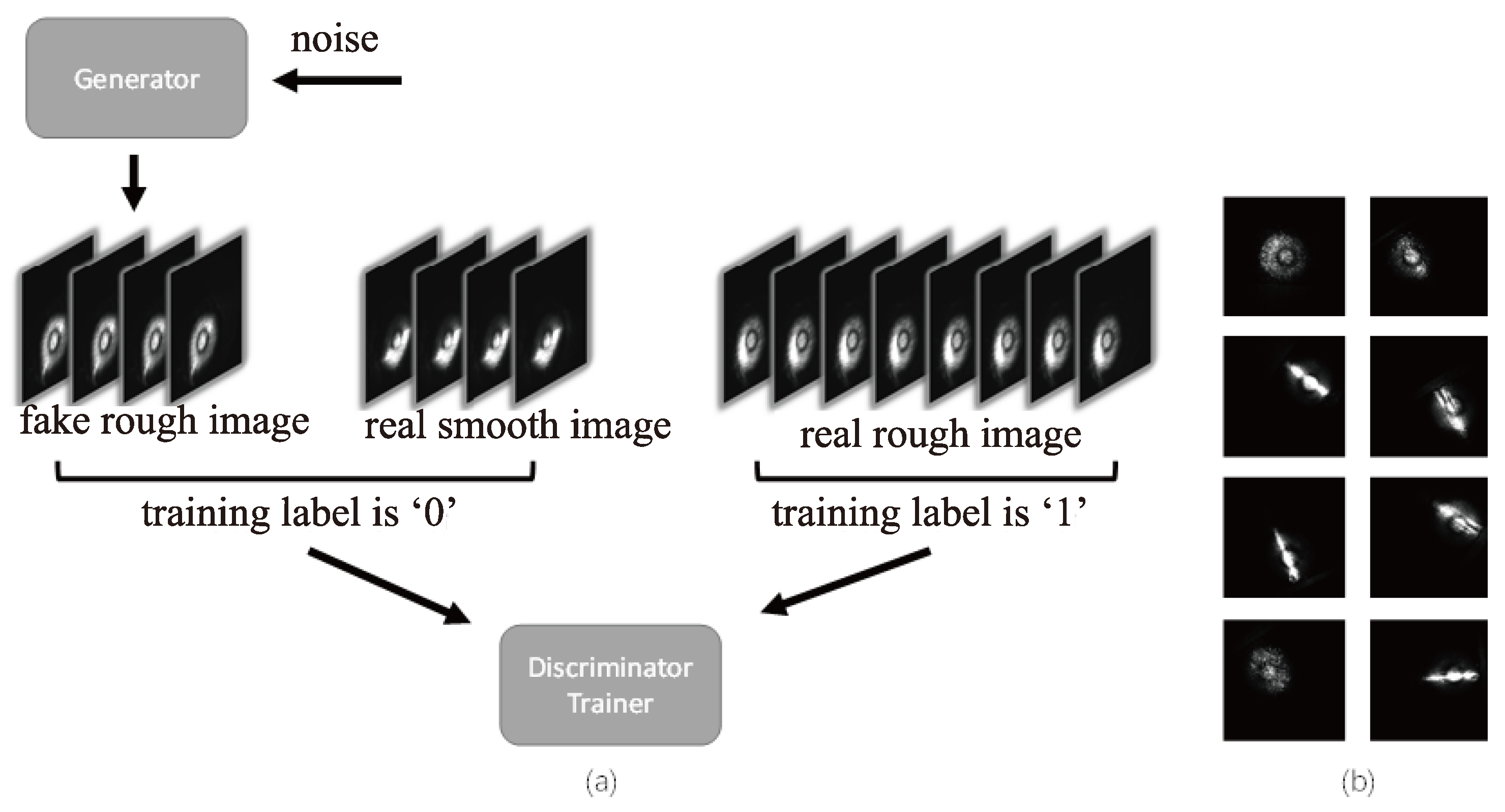
To teach the GAN the meaning of “rough,” real smooth images are added as fake data to train the discriminator along with the output of the generator, as shown in
Figure 6a.
Figure 6b shows examples of the surface roughness of workpieces generated by the GAN.
The GAN is trained using the expanded datasets, and then the GAN is able to generate a series of smooth and rough images as the training set. The problem is treated as a binary classification problem using the sigmoid function as the output activation function and the binary cross-entropy as the loss function for training, with the rough images labeled ‘1’ and the smooth images labeled ‘0’. In this method, the same network structure of the classifier with the discriminator of the GAN is used, as shown in
Table 1.
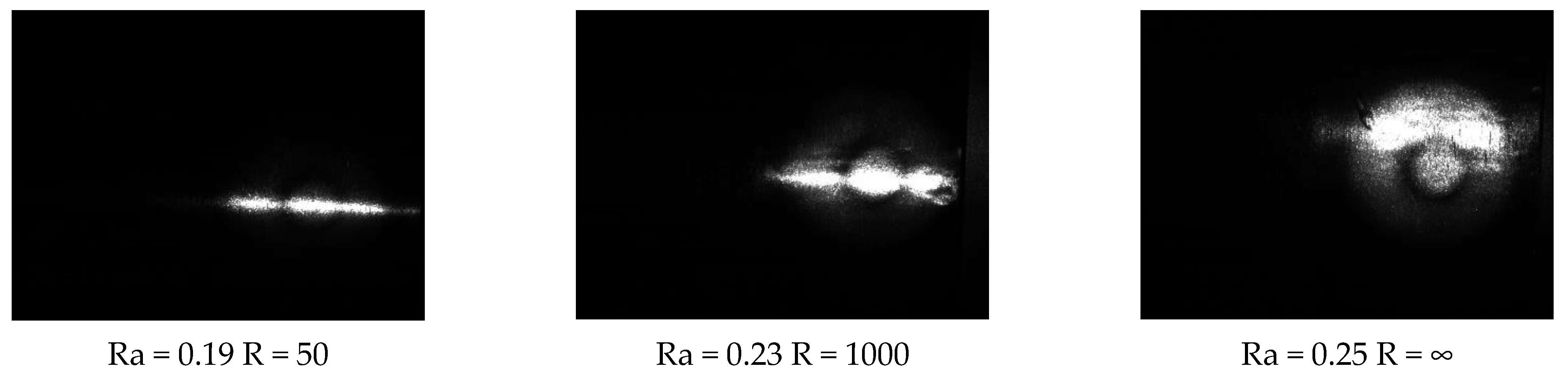
In the method described above, a dataset with only roughness Ra of 0.2, 0.4, 3.2, 6.3 and radius of curvature R of 50, 1000, and infinity are used as the training set. However, the dataset in the actual test contains more cases of roughness and radius of curvatures. A qualified classifier should be able to accurately distinguish the cases which are not encountered in the training set. Some of the actual test results are shown in
Table 2, which visually reflects the classifier’s scoring of images with different roughness levels. The smaller score means the smoother surface. The test results show that the method can accurately determine the untrained intermediate roughness (0.8 and 1.6 are the untrained cases), which indicates that the network can understand the concept of “roughness.”
4. Discriminating Method of Workpiece Surface Roughness
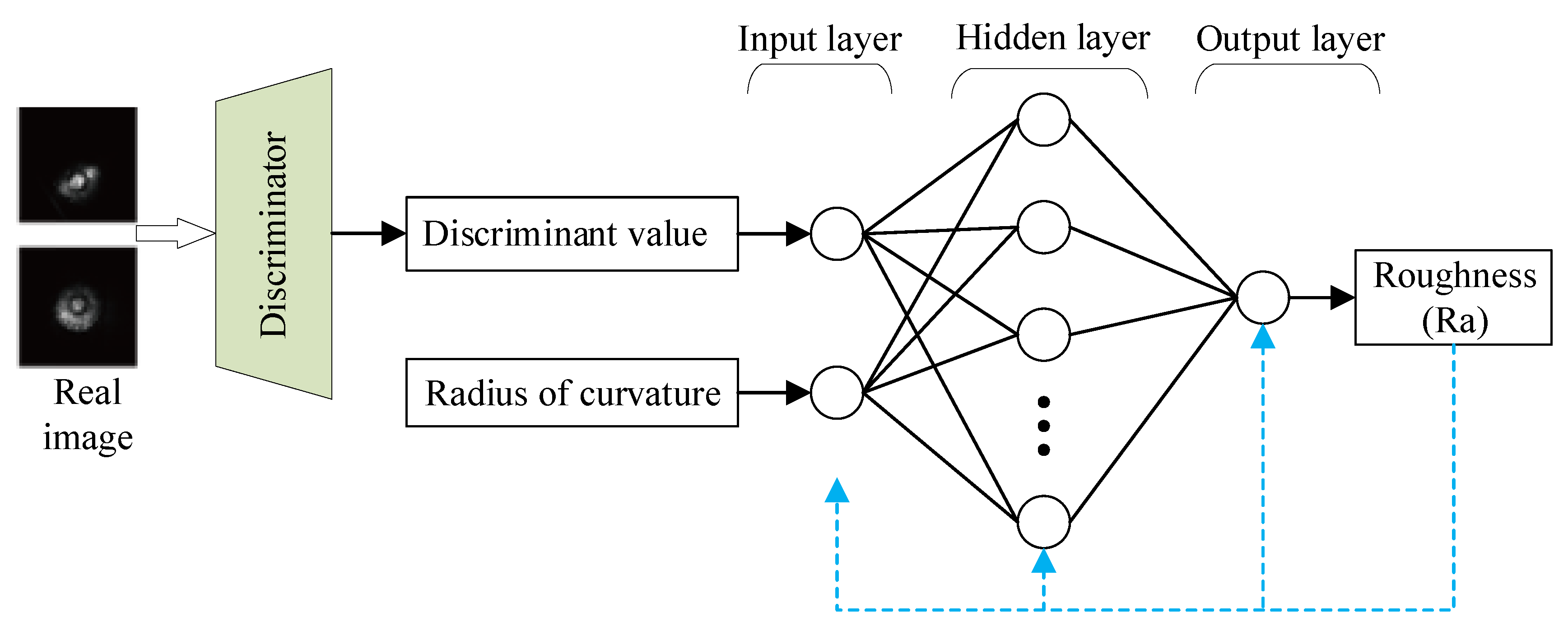
Roughness (Ra) is a small-distance (usually less than 1 mm) peak–valley that forms from a microgeometric shape error of the surface of the part. As shown above, the real surface image can obtain a discriminant value, nonlinearly related to roughness Ra through the trained GAN. In order to establish a mapping relationship between the discrimination value of GAN and surface roughness Ra, this paper proposes a surface roughness Ra discrimination method based on the BP neural network, which is shown in
Figure 7.
The input layer of the BP neural network for image discriminant value and radius of curvature is denoted as
, and the output surface roughness is denoted as
. The number of neurons in the hidden layer is
s, denoted as
. The bias value of the hidden layer is
, and the bias of the output layer is
.
denotes the connection weights from the input layer to the hidden layer,
denotes the connection weights from the hidden layer to the output layer, while
and
are the activation functions of the hidden and output layers, respectively. The forward propagation process of the BP neural network is expressed as:
Equation (8) completes the mapping from
to
.
denotes the target value of the output, and the error of the BP neural network is:
The error back-propagation process of the BP neural network is implemented by minimizing the objective function by Equation (9). The weights and biases of each layer are adjusted for each propagation as follows:
From Equation (8), it can be seen that the data transfer process between the layers is transformed and connected by the activation function. Meanwhile, in the error back-propagation process in the BP neural network in Equation (10), the derivatives of the activation function adjust the connection weights of each layer to reduce the error to the desired range. Considering the requirement that the activation function be continuously differentiable, the sigmoid function is chosen as the output layer activation function, and the tanh function is chosen as the output layer activation function.
To ensure accuracy of roughness estimation, this study determines the number of neurons in the hidden layer according to the Hecht–Nelson method [
29] because the hidden layer affects the stability of the network. The number of input layer neurons is n, while the number of hidden layer neurons is 2n + 1. That is, the number of hidden layer neurons in the network is 5. Networks with different numbers of neurons have also been tested, as shown in
Table 3.
After determining that there should be one hidden layer for the BP neural network model, the number of neurons in the hidden layer must be determined. For each neural network model in
Table 3, the average error between the actual and predicted values were recorded in 10 training sessions. It is clear from
Table 3 that as the number of neurons in the hidden layer increases, the accuracy does not necessarily follow. When the number of hidden layer neurons increases from 3 to 5, the average error decreases from 12.42% to 6.24%. However, as the number of hidden layer neurons continues to increase to 7, the average error increases from 6.24% to 14.63%. The 2-5-1 neural network structure has the smallest error, and so this network structure is used in the real-time surface roughness model in this study.
5. Experiments
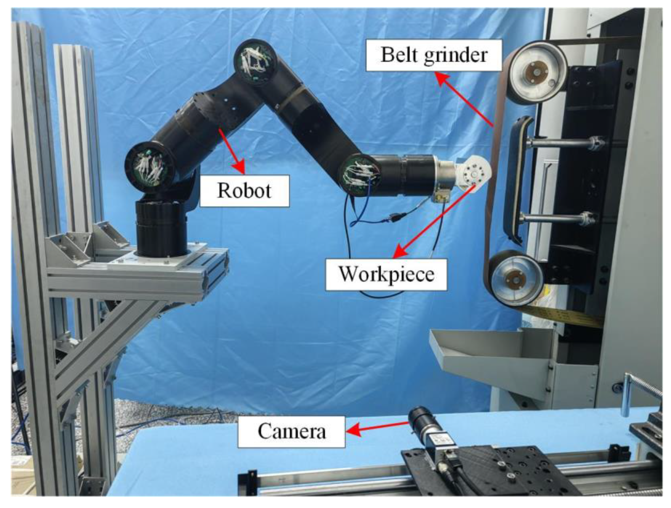
In this study, a robot is used to hold the workpiece while grinding a complex, curved item. The robotic grinding platform is built as shown in
Figure 8, consisting of a belt grinder, a lightweight robot with seven degrees of freedom and a camera.
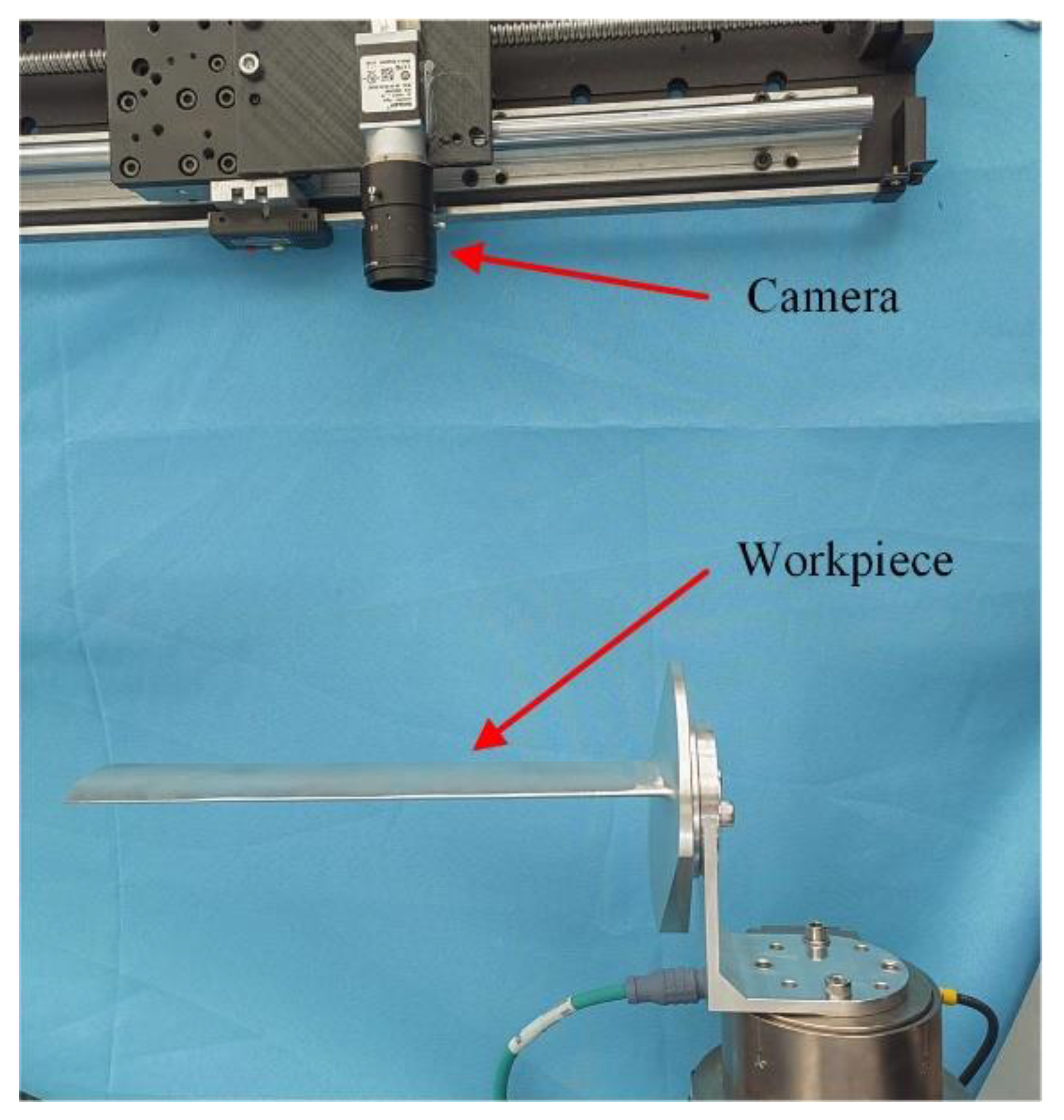
Surface roughness is a key feature of the surface texture of a workpiece because it has a significant impact on the service life and reliability of a mechanical product. This paper proposes a vision-based roughness measurement method for comprehensively considering the cost, usability, and efficiency. This method consists of three stages: image acquisition, self-supervised learning and result discrimination. A narrow-angle industrial camera is used to build a vision-based surface roughness measurement system, as shown in
Figure 9.
The narrow-angle Balser ace 2 industrial camera meets the needs of this method for surface roughness measurement of curved workpieces. Its detailed parameters are shown in
Table 4.
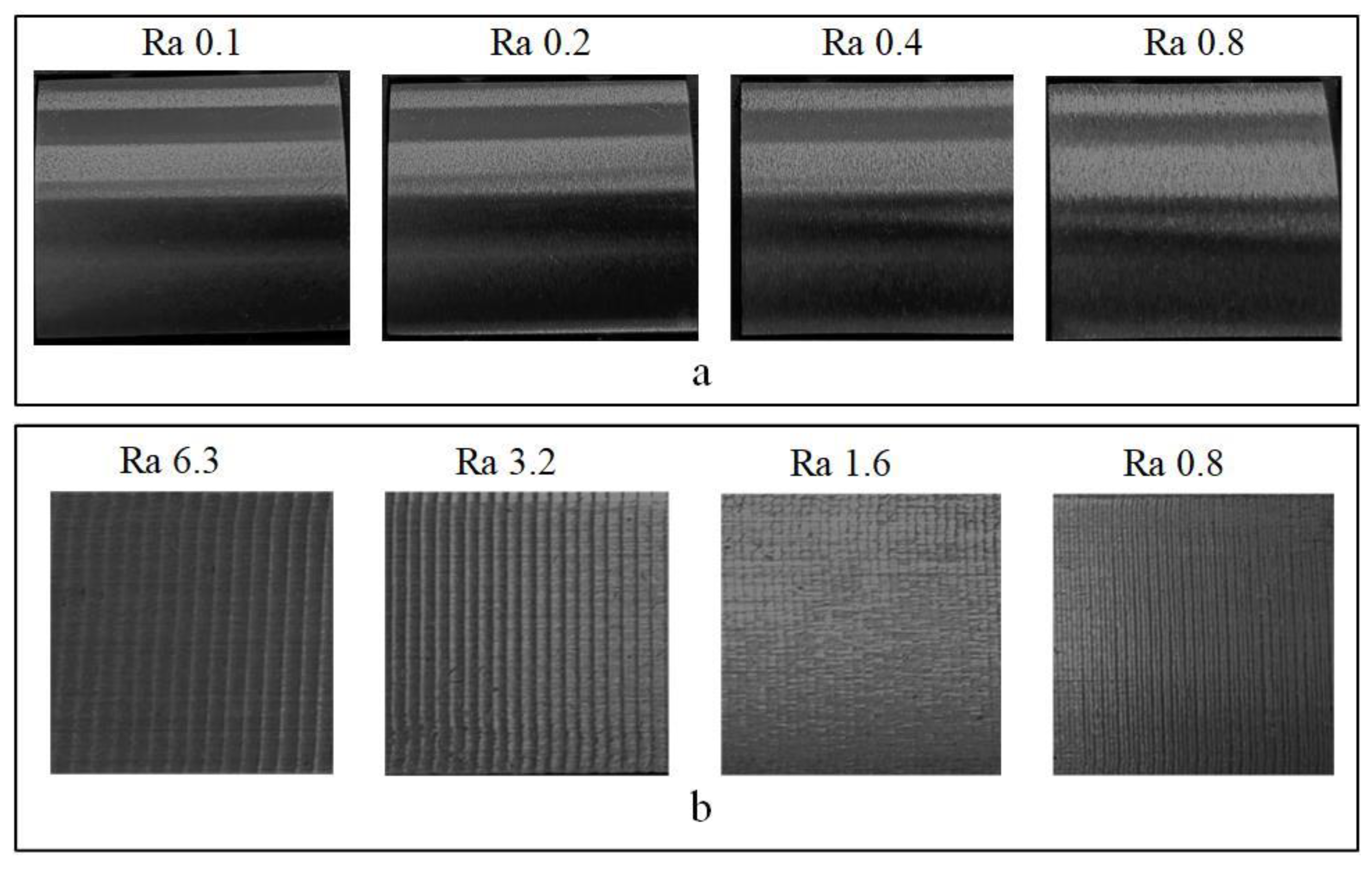
Balser ACE 2 samples images of standard grinding surface roughness contrasts as shown in
Figure 10a, and images of standard milled surface roughness contrasts as shown in
Figure 10b. There is no significant difference between images Ra 0.2 and Ra 0.1. The camera can distinguish surfaces with surface roughness Ra greater than 0.2. The image samples in
Figure 10 are added to the training set of the proposed GAN to enrich the samples and increase the measurement accuracy of the model.
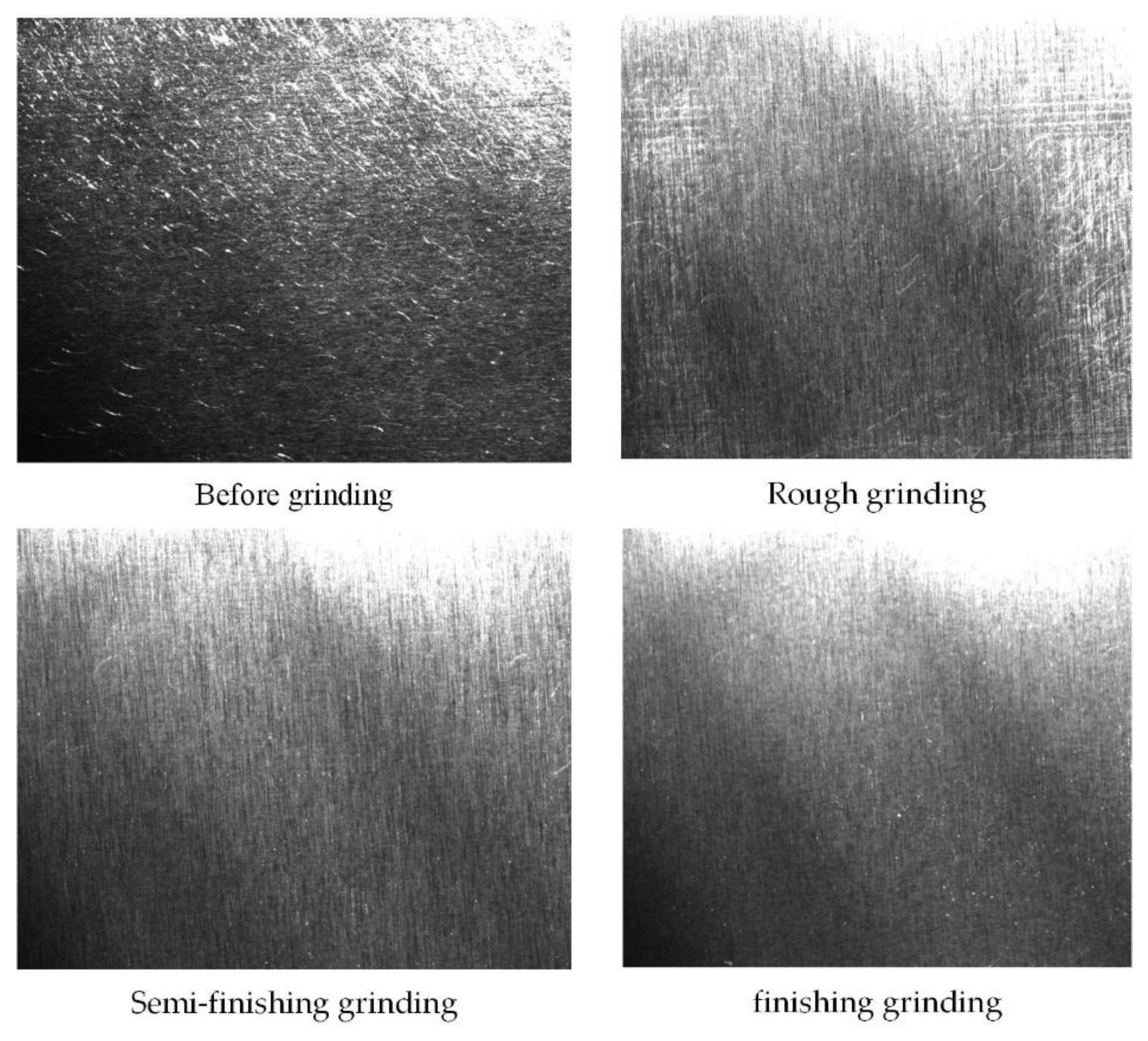
The blade-grinding process is divided into three processing stages according to the requirements of the grinding process: rough grinding, semi-finishing grinding and finishing grinding. The rough grinding stage removes a large amount of the material using the grinding parameters belt line speed 5 m/s, feed speed 3 mm/s, belt mesh 120 and contact force 15 N. The semi-finishing stage removes a small amount of material with the grinding parameters of belt line speed 5 m/s, feed speed 3 mm/s, belt mesh 320 and contact force 10 N. The finishing stage is mainly for finishing the surface of the workpiece with the grinding parameters belt line speed 5 m/s, feed speed 3 mm/s, belt mesh 320, and contact force 5 N. After each grinding stage, the surface roughness is measured and analyzed.
In this study, an industrial camera was used to take pictures of the workpiece surface under a specific light environment to measure the surface roughness conditions, as shown in
Figure 11. In order to compare the measurement accuracy of different learning algorithms, ANN and CNN are added to train the surface roughness measurement model in this paper. The GAN-BPNN, ANN, CNN were used to judge the smoothness of the polished processing surface in
Figure 11, as shown in
Table 5. The proposed GAN-BPNN has a margin of error of 10%. However, the prediction error of ANN and CNN were more than 10%.
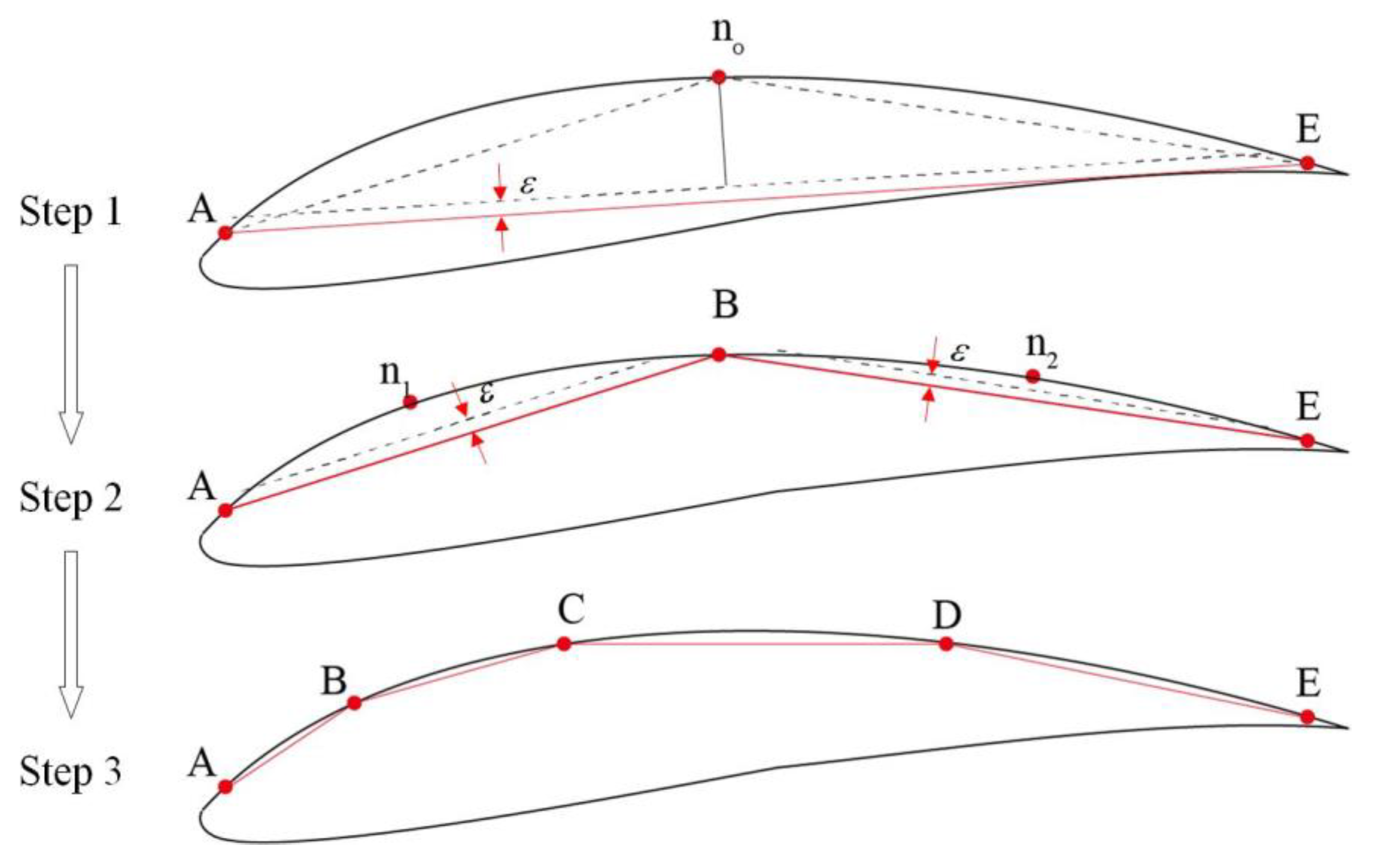
In order to measure blade surface roughness more accurately, this paper designs a sampling point distribution method based on constant chord height. The method realizes a dense distribution of sampling points in the region with a large curvature variation and a sparse distribution in the region with a small curvature variation, as shown in
Figure 12.
(1) Set a chord height .
(2) The baseline AE was obtained by connecting the end points of the curve.
(3) Determine whether there exists a point on the curve whose distance to the datum line is greater than . If there is a point on , whose distance from the datum line AE is the farthest point is , then delete the original datum line AE.
(4) Set to B and connect the AB and BE as the new datum line.
(5) Determine whether there exists a point on the curve whose distance to the datum line is greater than , and if there is a point on whose distance from the datum line AB is the farthest point is . Similarly, point on curve is obtained. Rewrite A, , B, , E as A, B, C, D, E.
Repeat the above process until all points on the curve to the datum line position are less than the threshold
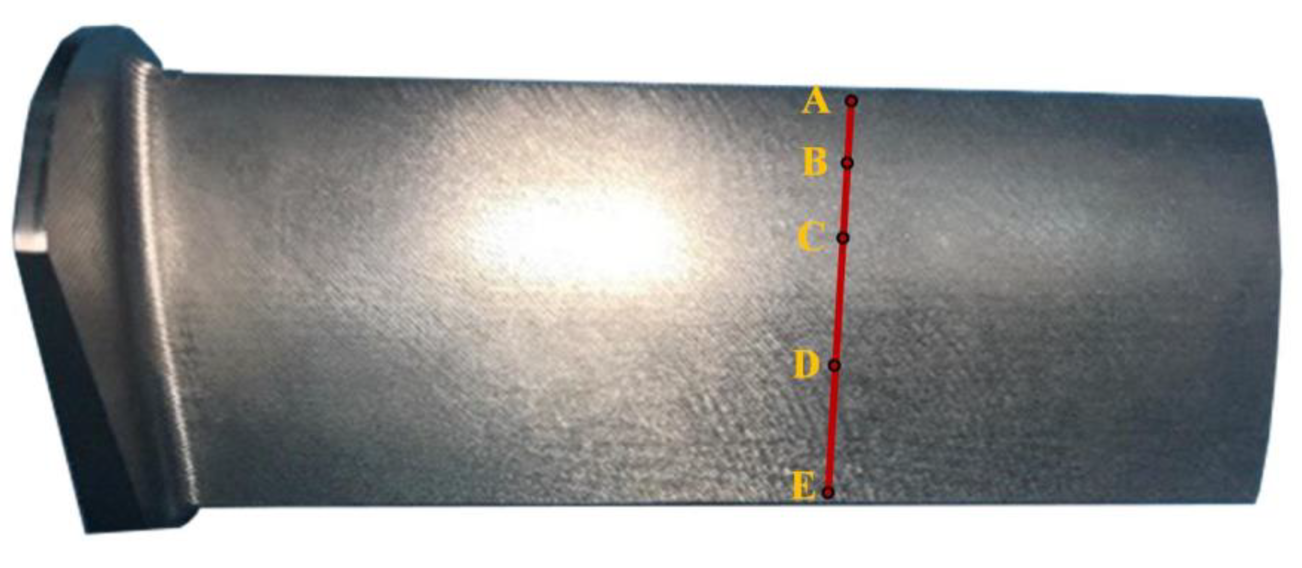
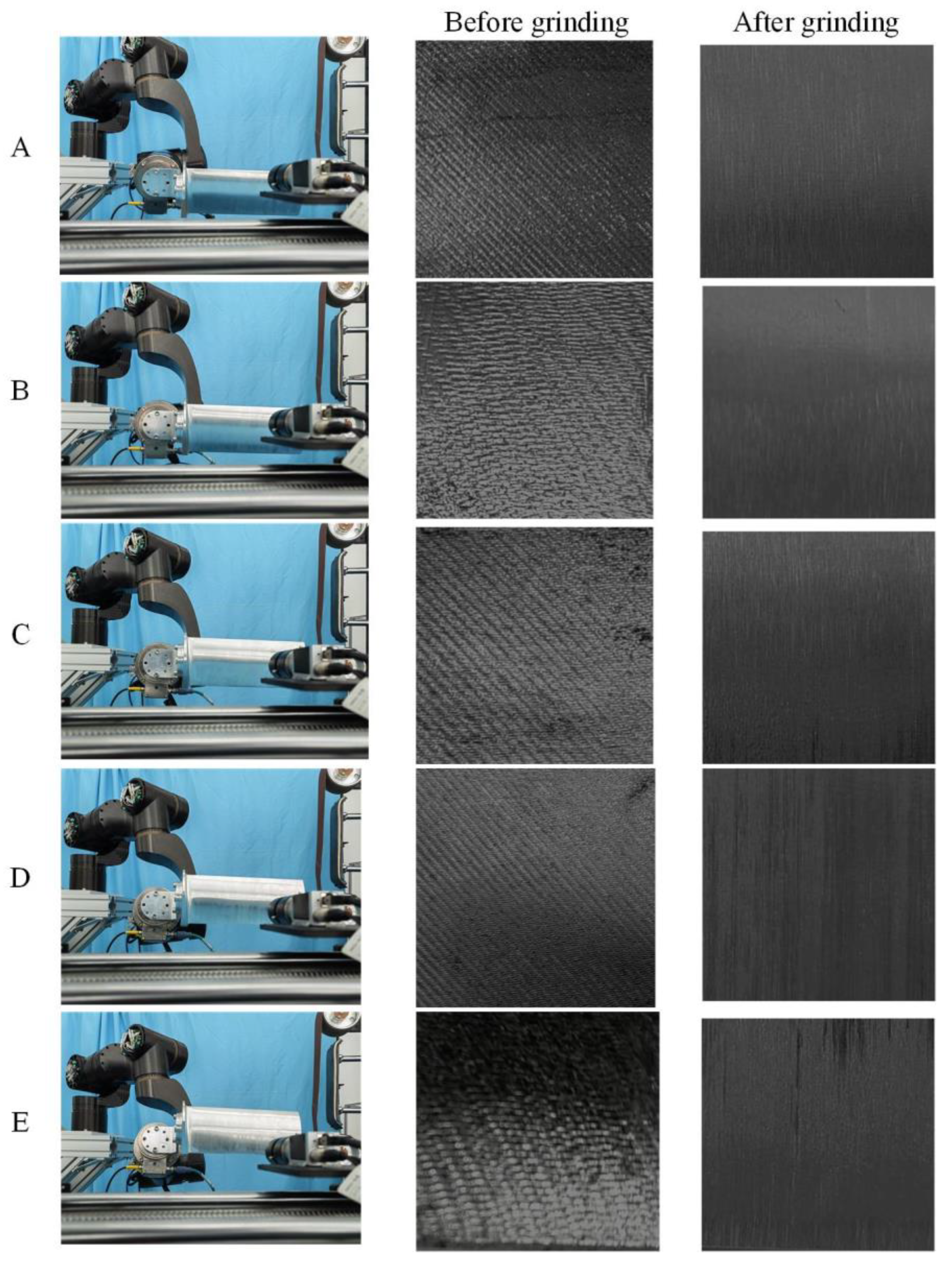
. In this paper, five sampling points (A,…, E) marked in the figure were taken as examples to compare the roughness changes of blades before and after grinding, as shown in
Figure 13. The robot planed the motion trajectory according to the position and curvature of the sampling points (20 mm × 20 mm area centered on this point), collecting images of the five sampling points in turn at the best angle, as shown in
Figure 14.
The image data of the sampling points before and after polishing can obtain the corresponding predicted value by the roughness discrimination model of the GAN + BP neural network, as shown in
Table 6. It can be seen that the relative error between the predicted roughness and the real roughness (measured by SJ-210) has a margin of error of 10%, which meets the needs of industrial detection.
6. Conclusions
In this paper, we propose a roughness evaluation method combining generative an adversarial network (GAN) and a BP neural network, which avoids the influence of surface image differences with different curvatures on the accuracy of roughness measurements. The method automatically learns features in the image by generators playing with discriminators, eliminating the independent feature extraction step. This does not merely shorten the prediction time but reduces the complexity of model training as well. Experiments show that the proposed method can measure a free-form surface with a minimum roughness of 0.2 µm, and measurement results have a margin of error of 10%. Since the proposed method does not require the operator to have the field knowledge of feature recognition, the method is easier to apply in a factory. However, the proposed roughness evaluation method using GAN takes a long time for model training due to its convolution process and depth structure characteristics. To overcome this problem, the adaptive model can be considered in future research to automatically adjust the hyperparameters.


