Mobile Robots—AHP-Based Actuation Solution Selection and Comparison between Mecanum Wheel Drive and Differential Drive with Regard to Dynamic Loads

Abstract

Mobile robots are increasingly used in industrial applications. There are many constructive solutions for mobile robots using various variants of actuation and control. The proposed work presents a low-cost variant of a mobile robot equipped with Mecanum wheels, which uses brushed DC motors, controlled by the PWM method as the actuation solution. In the first part, a multicriteria analysis based on the AHP method was performed for the selection of the actuation solution. Then, using the software tools Simscape Multibody, Matlab, and Simulink, models were developed that allowed the simulation of the operation of the proposed robot, based both on its kinematics and dynamics. Using these models, both the Mecanum wheel drive version and the differential drive version were studied by means of simulation. The simulations mainly aimed at identifying the way the currents vary through the wheel drive motors, in order to find methods to reduce them. The values obtained by the simulation were later compared with those obtained experimentally, and the corresponding conclusions with regard to the accuracy of the models were drawn.

1. Introduction

Industrial autonomous mobile robots are increasingly used in industrial applications [1]. The development of electric battery technology, as well as inexpensive control solutions based on microcontrollers have favored this.

The structure of mobile robots, mainly the use of Mecanum wheels to improve the maneuverability of the robotic structure, has been the subject of intensive research recently [2,3,4]. However, differential drive steering, which uses normal wheels, is still considered an efficient solution for mobile robots [5,6,7,8,9].

Path planning [10,11,12] and trajectory control (including obstacle avoidance) for mobile robots have also been considered as important research topics in the field of mobile robots. Classical PID algorithms [13] together with advanced control algorithms for this purpose are reported in the literature.

The work described in [14,15] used an internal terminal sliding mode algorithm for trajectory-tracking control of a mobile robot using Mecanum wheels. The research in [16] presented the implementation of a robust sliding mode controller on a Mecanum-wheeled robot to control the trajectory in the presence of uncertainties. Neural tracking control for the same type of mobile robot was presented in [17]. Advanced control methods have been used for mobile robots using differential drive steering, and the work presented in [18] introduced a fuzzy logic controller for this purpose.

Simulating the movement and behavior of mobile robots is also an important topic, which has been tackled by recent research. The work presented in [19] introduced a simulation using Unity3D of a mobile robot using Mecanum wheels.

However, the dynamic analysis [20] of mobile robots is not so often tackled in the literature.

With regard to the actuation solutions, the choice is limited by the fact that most mobile robots are also autonomous, so there is the matter of using DC batteries as the power source. Thus, the main solutions for actuating mobile robots are brushed DC motors, controlled by means of the PWM method [4,20], brushed DC servomotors [9], brushless DC servomotors [16,17], and stepping motors [21,22].

It can be concluded that most of the mobile robot solutions use complex constructive and actuation solutions, mainly oriented towards performance, without much consideration of the high prices they can reach. Advanced path planning and obstacle avoidance solutions coupled with advanced control algorithms can result in advanced performance that far exceeds real industry requirements. The present work aims to implement a low-cost mobile robot solution, but with average performance, capable of being expanded later. The research sought to justify the choice of a simple actuation solution, based on DC motors with brushes, controlled by the PWM method, using Arduino boards, as well as the development of models that allow the study through kinematic and dynamic simulation of the behavior of the proposed robot.

Mobile robot health monitoring and fault diagnosis of actuators have also been topics addressed by recent research. In the work presented in [23], actuator faults were considered as the loss of efficiency of actuators because of wear. However, there are no references on how the peak currents occurring during different operating regimes and different types of traveled trajectories can affect the lifetime of mobile robot actuators and how these current peaks can be reduced.

A study on the influence of the types of trajectories (linear or curved) on the energy consumption of mobile robots was presented in [24]. A theoretical model (validated experimentally) was proposed that allowed the evaluation of the energy consumption depending on the type of trajectory traveled. Even in this case, the maximum values of the current through the wheel drive motors and how the types of trajectories influence these maxima were not taken into account.

A fault-tolerant control scheme for a four-wheel Mecanum mobile robot was presented in [25]. It allowed controlling the robot while avoiding obstacles and taking into consideration the motor limits. However, the proposed scheme, tested by simulations, was not validated by experimental tests.

Another control algorithm, for differentially driven mobile robots, which took into consideration the motor limits, was presented in [26,27], but this was also tested only by simulation.

It can be noticed that many of the works presented in the literature use the MATLAB-Simulink software package as a tool for modelling and simulation [24,27]. However, the models used are not made available to the readers. Moreover, new tools have appeared in MATLAB (Simscape), which allow the integration of geometric CAD 3D models of robots with relations describing their kinematic and dynamic models, but their use has not yet been reported.

2. Materials and Methods

2.1. AHP Analysis for the Actuation Solution

The approach in this work was to develop a low-cost, yet efficient, autonomous mobile robot, suited for industrial applications. Thus, the developed platform will move inside a controlled environment, transferring parts between workplaces. Consequently, the paths are fixed, and the possibilities of obstacle occurrence are rather small. Therefore, path planning, trajectory accuracy, and obstacle avoidance are not so important for the proposed autonomous mobile robot.

In order to select the actuation solution for the proposed platform, a multi-criteria decision-making method, based on the analytic hierarchy process (AHP) [28,29,30], was used.

Three actuation solutions were considered:

• DCSERVO—a system using either a brushed or a brushless DC servomotor, with closed-loop control. This system includes main position feedback and secondary velocity feedback, with position and speed sensors. The control is based on PID algorithms (or more advanced ones), and the system controllers can be tuned by the user to optimize the behavior of the system;
• DCPWM—a system using a brushed DC motor, commanded through variable-width voltage pulses, by means of the pulse with modulation (PWM) method. This system does not include any feedback, and it allows the variation of the motor speed in a discrete manner (between standstill and maximum speed), without the possibility of setting a velocity profile;
• STEPPER—a system using a stepping motor, commanded by means of voltage pulses. The system does not include feedback devices, but allows the user to control both the position of the motor shaft (by controlling the number of pulses) and the speed (by controlling the pulse frequency).

The actuation solutions described above were analyzed using the following criteria:

• C1—control performance: This criterion considers the possibilities of compensating the system errors while the system is working (feedback), the overall accuracy of the system and how the user can improve it by tuning the system parameters, as well as the possibility of programming the velocity profiles in order to avoid high acceleration and to reduce the jerk phenomenon;
• C2—ease of implementation: This criterion considers the complexity of the system (how many components are required, how complex the control software is, how much expertise is required for implementation, and how much time is required for implementation);
• C3—costs: This criterion is self-explanatory; it considers the overall costs of the system;
• C4—energy efficiency: This criterion considers how much energy each actuation system requires during operation.

The AHP method involves the pairwise comparison of the selected criteria with each other. The judgement scale proposed in [28] was used for the comparisons: 1—equally important; 3—weakly more important; 5—strongly more important; 7—demonstrably more important; 9—absolutely more important. The values in between (2, 4, 6, and 8) represent compromise judgements.

Table 1. Preference matrix A.

	C1	C2	C3	C4
C1	1	1/3	1/3	1/2
C2	3	1	3	3
C3	3	1/3	1	3
C4	2	1/3	1/3	1

, also called according to the AHP methodology the preference matrix, gives the results of the comparisons.

For example, in Table 1, on the first line, the control performance (C1) was considered weakly more important than the ease of implementation (C2) and the costs (C3), while the same criterion (C1) was considered as slightly equal, but somewhat less than the criterion related to the energy efficiency.

Here, we considered the fact that mobile robots used for industrial applications are mostly used for the interoperation transfer of parts (moving parts form one workstation to another), along known (and mostly unchanged) trajectories; thus, the control performance of the mobile platform is not so important in this context.

Following the AHP methodology, it is necessary to normalize matrix A and transform it into matrix B, using the following relation:

$$B=[b_{ij}] where b_{ij}=\frac{a_{ij}}{{\displaystyle \sum _{i=1}^n{a}_{ij}}},$$

(1)

After that, the eigenvector w = [w_i] has to be calculated according to the following:

$$w_{ij}=\frac{{\displaystyle \sum _{i=1}^n{b}_{ij}}}{n},$$

(2)

Matrix B is presented in

Table 2. Matrix B normalized.

	C1	C2	C3	C4	w
C1	0.1111	0.1658	0.0708	0.0667	0.1036
C2	0.3333	0.5025	0.6438	0.4000	0.4699
C3	0.3333	0.1658	0.2146	0.4000	0.2784
C4	0.2222	0.1658	0.0708	0.1333	0.1481

, where, in the last column, the eigenvector w was introduced.

The pairwise comparisons have to be checked for consistency by calculating the maximum eigenvalue [23,24,25]:

$${\lambda }_{max}=\frac{1}{n}\sum _{i=1}^n\frac{{\left(Aw\right)}_i}{w_i}=4.2046andCI=\frac{{\lambda }_{max}-n}{n-1}=0.0766,$$

(3)

where λ_max is the matrix’s largest eigenvalue and CI the consistency index.

The following step involves the calculation of the consistency ratio, using

Table 3. Values of the consistency indexes [28].

Size of Matrix (n)	1	2	3	4	5	6	7	8	9	10
Random average CI (r)	0	0	0.52	0.89	1.11	1.25	1.35	1.40	1.45	1.49

, which is called the random consistency index table [28]. It can be noticed that for a 4-dimensional matrix, one has to choose 0.89 for the r coefficient.

$$CR=[({\lambda }_{max}-n)/\left(r\left(n-1\right)\right)]·100\%=7.66\%,$$

(4)

According to Relation (4), where CR is smaller than 10%, the consistency of the pairwise comparisons is confirmed. The next step of the AHP process involves the evaluation of the three actuation solutions with respect of the four proposed criteria. The result of the evaluation is presented in

Table 4. Pairwise comparison of the actuation solutions (criterion C1).

C1	DCSERVO	DCPWM	STEPPER	w
DCSERVO	1	5	3	0.6484
DCPWM	1/5	1	1/2	0.1223
STEPPER	1/3	2	1	0.2293

,

Table 5. Pairwise comparison of the actuation solutions (criterion C2).

C2	DCSERVO	DCPWM	STEPPER	w
DCSERVO	1	1/7	1/5	0.0733
DCPWM	7	1	3	0.6443
STEPPER	5	1/3	1	0.2824

,

Table 6. Pairwise comparison of the actuation solutions (criterion C3).

C3	DCSERVO	DCPWM	STEPPER	w
DCSERVO	1	1/5	1/3	0.1060
DCPWM	5	1	3	0.6340
STEPPER	3	1/3	1	0.2600

and

Table 7. Pairwise comparison of the actuation solutions (criterion C4).

C4	DCSERVO	DCPWM	STEPPER	w
DCSERVO	1	3	5	0.6340
DCPWM	1/3	1	3	0.2600
STEPPER	1/5	1/3	1	0.1060

. Each of the tables from 4 to 7 also gives in the last column the eigenvector values.

In Table 4, on the first line, considering the control performance (C1 criterion), the DCPWM solution is strongly more important than the DCPWM solution and weakly more important than the STEPPER solution. Remember that DCSERVO includes feedback loops and tunable controllers, which allow a much higher degree of control of the motor speed and position than DCPWM situation. Furthermore, the STEPPER solution allows the user to continuously command the speed and position of the motor by changing the frequency and number of voltage pulses fed to the motor, a solution not so performant as DCSERVO, but significantly better than DCPWM, from the control performance point of view.

In Table 5, on the first line, taking into consideration the ease of implementation (C2 criterion), the DCPWM solution is demonstrably more important than the DCSERVO solution and strongly more important than the STEPPER solution. Consider that DCSERVO is a much more complex solution, with a significantly higher number of components (due to the feedback loops), and its implementation requires, among others, the tuning of the controllers. Similarly, the STEPPER solution, while not so complex as DCSERVO, also requires an implementation process that is much complex than the one required by the DCPWM solution.

Using the data from Table 4, Table 5, Table 6 and Table 7, the C matrix was built. In its columns, the C matrix gives the eigenvectors of the pairwise comparisons of the proposed actuation solutions. It is here noticeable that the order of the columns of matrix C is imposed by the order of the criteria resulting from Table 2: C2, C3, C4, and C1. After building matrix C, it is multiplied by the preference vector w, thus obtaining the preference vector x of the actuation solutions:

$$x=Cw=\left[\begin{array}{c}0.0733 0.1060 0.6340 0.6484\\ 0.6443 0.6340 0.2600 0.1223\\ 0.2824 0.2600 0.1060 0.2293\end{array}\right]\left[\begin{array}{c}0.1036\\ 0.4699\\ 0.2784\\ 0.1481\end{array}\right]=\left[\begin{array}{c}0.3299\\ 0.4552\\ 0.2149\end{array}\right],$$

(5)

By analyzing Relation (5), the results of the AHP process indicate that DCPWM is the most advantageous solution, followed by DCSERVO and STEPPER.

Finally, again, the main purpose of the considered mobile robot is for industrial applications, a factor that favored the prevalence of a low-cost actuation solution.

2.2. The Mobile Robot

A mobile robot platform with Mecanum wheels was developed for this research and is presented in Figure 1.

Each wheel can be actuated independently using DC motors commanded through variable-width voltage pulses, by means of the pulse with modulation (PWM) method.

DCX 22 L DC motors from Maxon (Maxon Motor AG, Sachseln, Switzerland) were used as the actuation motors. Two Arduino Mega 2560 boards (Arduino AG, Italy) were used to handle the generation of the variable-width voltage pulses for the actuation motors. Two motor drivers dual, VNH5019, were used to command the drive motors of the wheels (Pololu, Las Vegas, NV, USA).

The platform was also equipped with various sensors, such as ultrasonic distance sensors and an infrared sensor module for obstacle avoidance, but these sensors were not used during the tests presented in this paper

2.3. Considered Kinematic Solutions

To test the operation of the mobile platform, two kinematic solutions were considered: four-wheel Mecanum and differential drive.

2.3.1. Four-Wheel Mecanum Kinematics

The kinematic solution for a four-wheel Mecanum mobile robot was taken from the work presented in [31] and provided in the Mobile Robotics Simulation Toolbox [32] within Matlab software package (The MathWorks Inc., Natick, MA, USA).

A schematic diagram of the four-wheel Mecanum mobile robot is presented in Figure 2.

According to [26,27], the inputs of the kinematic model are the wheel speeds, from ω₁ to ω₄ (in rad/s), while the outputs are the linear velocities v_x and v_y (in m/s) and the angular velocity ω (in rad/s).

The forward kinematics can be described by the following relation:

$$\left[\begin{array}{c}{v}_x\hfill \\ v_y\hfill \\ \omega \hfill \end{array}\right]=\frac{R}{4}\left[\begin{array}{cccc}1& 1& 1& 1\\ -1& 1& 1& 1\\ -2/\left(L_x+L_y\right)& 2/\left(L_x+L_y\right)& -2/\left(L_x+L_y\right)& -2/\left(L_x+L_y\right)\end{array}\right]\left[\begin{array}{c}{\omega }_1\hfill \\ {\omega }_2\hfill \\ {\omega }_3\hfill \\ {\omega }_4\hfill \end{array}\right],$$

(6)

The inverse kinematics can be described by the following relation:

$$\left[\begin{array}{c}{\omega }_1\hfill \\ {\omega }_2\hfill \\ {\omega }_3\hfill \\ {\omega }_4\hfill \end{array}\right]=\left[\begin{array}{ccc}\hfill 1& \hfill -1& \hfill -\left(L_x+L_y\right)/2\\ \hfill 1& \hfill 1& \hfill \left(L_x+L_y\right)/2\\ \hfill 1& \hfill 1& \hfill -\left(L_x+L_y\right)/2\\ \hfill 1& \hfill -1& \hfill \left(L_x+L_y\right)/2\end{array}\right]\left[\begin{array}{c}{v}_x\\ v_y\\ \omega \end{array}\right],$$

(7)

2.3.2. Differential Drive Kinematic

The kinematic solution for the differential mobile robot was taken from the one provided in the Mobile Robotics Simulation Toolbox [32] in the Matlab software package (The MathWorks Inc., Natick, MA, USA).

A schematic diagram of the differential drive mobile robot is presented in Figure 3.

According to [32], the inputs of the kinematic model are the left and right wheel speeds, ω_L and ω_R (in rad/s), while the outputs are the linear velocity v (in m/s) and the angular velocity ω (in rad/s).

The forward kinematics can be described by the following relation:

$$v=\frac{R}{2}\left({\omega }_R+{\omega }_L\right), \omega =\frac{R}{L}\left({\omega }_R-{\omega }_L\right),$$

(8)

The inverse kinematics can be described by the following relation:

$${\omega }_L=\frac{1}{R}\left(v-\frac{\omega L}{2}\right), {\omega }_R=\frac{1}{R}\left(v+\frac{\omega L}{2}\right),$$

(9)

2.4. Simulation

The Matlab software package (The MathWorks Inc., Natick, MA, USA), with the Simulink and Simscape Multibody modules, was used for the simulations. The Simscape Multibody module allows the user to integrate the 3D CAD model into the dynamic simulation of the system.

Consequently, the 3D model of the mobile robot, given in Figure 4, was built using the Solidworks software package (Dassault Systemes, Vélizy-Villacoublay, France).

The next step involved the exporting of the 3D CAD model (structured as an assembly of parts) of the mobile robot from Sollidworks to Simscape, by using the Simscape Multibody Link Plug-In provided by Mathworks and installed in the external CAD application (Solidworks). The result of this operation was an xml file, which was further imported into the Simscape Multibody, generating a combined Simulink/Simscape simulation diagram.

The simulation diagram of the mobile robot, considering the four-wheel Mecanum kinematic solution, is presented in Figure 5. The diagram also uses the block from the Mobile Robotics Simulation Toolbox [32] within Matlab. The mechanical dependencies between forces acting on the chassis of the robot and torques acting on the wheels, also considering the harmonic drive gear ratio of the motor/wheel, were introduced in the simulation diagram.

Table 8. Parameters of the system used for the simulation.

Parameter	Value
Motor parameters
Nominal voltage (V)	12
Nominal speed—n (rpm)	10,700
Nominal torque (mNm)	30.05
Nominal current (A)	3.21
Stall current (A)	35.8
Torque constant—Kt (Nm/A)	0.00973
Speed constant—Kv (Vs/rad)	0.00973
Harmonic drive gear ratio—N	200
Mobile robot parameters
Wheel radius (m)	0.05
Wheelbase (m)	0.2
Track (m)	0.2

presents the values of the physical parameters of the system used for the simulation.

Figure 6 presents the simulation diagram for the differential drive kinematic solution.

The Matlab function “Jacobian” transpose from the diagram presented in Figure 6 was introduced in order to calculate the torques acting on the mobile robot wheels, according to the relations presented below.

The overall force acting at the level of the planar joint can be expressed in the following matrix form:

$$F=\left[\begin{array}{c}{F}_x\\ F_y\\ M\end{array}\right],$$

(10)

where F_x and F_y are the forces acting on the X and Y axis and M is the torque acting around the Z axis of the planar joint.

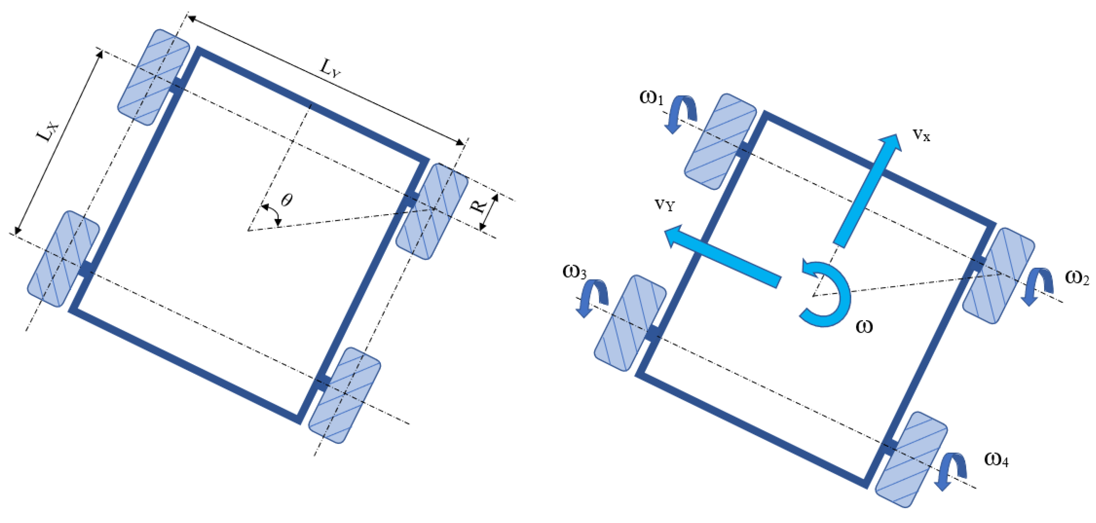
Thus, the transposed Jacobian matrix can be defined as:

$$J^T=\left[\begin{array}{cc}\frac{R_w}{2}\cos \theta & \frac{R_w}{2}\sin \theta \frac{R_w}{2}L\\ \frac{R_w}{2}\cos \theta & \frac{R_w}{2}\sin \theta -\frac{R_w}{2}L\end{array}\right],$$

(11)

where R_w is the radius of the wheel, L the wheelbase, and θ the orientation angle of the mobile robot.

Thus, the following relation can be written:

$$M_t=J^T·F,$$

(12)

where M_t is the overall torque acting on the mobile robot.

Taking into consideration that M_t is distributed on the wheels, on the left side and on the right side, the following relation can also be written:

$$M_t=\frac{1}{2}\left[\begin{array}{c}{M}_r\\ M_l\end{array}\right],$$

(13)

where M_l stands for the torque on the left-side wheels (wheels 1 and 3) and M_r stands for the torque on the right-side wheels (wheels 2 and 4). The 1/2 factor was introduced because the mobile platform has four wheels, instead of two.

Inputs and Simulation Results

The inputs of the simulation diagrams were the speed of the four wheels of the mobile robot. The inputs were generated by means of the pulse with modulation (PWM) method; thus, the speed of each motor varied in the form of pulses, with the maximum amplitude equal to the nominal speed of 10,700 rpm. Taking into account the gearbox transfer ratio between the motor and the wheel, the maximum speed of a wheel can be calculated as:

$$n_w=\frac{n}{N}=\frac{10700 rpm}{200}=53.5 rpm$$

(14)

The trajectory considered for the simulation was a square, with a side of approximately 900 mm. The accuracy of the length of the side is not so important, because the main goal of the simulations and the experiments was to determine the currents through the motors, which are influenced by the changes of direction, not by the length of the trajectory.

For the differential drive kinematic solution, two sub-cases were tackled. In the first sub-case, traversing the corners was achieved without generating a loop at the corner point, the mobile robot rotating around its center; see Figure 7a. The speed of the wheels on the left side (wheels 1 and 3), when traversing the corners, is equal and in the opposite direction to the rotation of the wheels on the right side (wheels 2 and 4). In the second case, cornering was achieved by generating a loop in the corner; see Figure 7b. In this situation, the rotation of the left-hand wheels is zero, with only the right-hand wheels turning.

The inputs for the three situations (four-wheel Mecanum, differential drive without a loop and differential drive with a loop) are presented in Figure 8, Figure 9 and Figure 10 and in

Table 9. Inputs for the four-wheel Mecanum kinematic solution—values.

	Wheel 1 Speed(rpm)	Wheel 2 Speed(rpm)	Wheel 3 Speed(rpm)	Wheel 4 Speed(rpm)
Line 1 (forward)	53.5	−53.5	−53.5	53.5
Line 2 (left)	53.5	53.5	−53.5	−53.5
Line 3 (backward)	53.5	53.5	−53.5	−53.5
Line4 4 (right)	53.5	−53.5	−53.5	53.5

,

Table 10. Inputs for the differential drive no-loop kinematic solution—values.

	Wheel 1 Speed(rpm)	Wheel 2 Speed(rpm)	Wheel 3 Speed(rpm)	Wheel 4 Speed(rpm)
Line 1 (forward)	53.5	53.5	53.5	53.5
Corner 1	−53.5	53.5	−53.5	53.5
Line 2 (left)	53.5	53.5	53.5	53.5
Corner 2	−53.5	53.5	−53.5	53.5
Line 3 (backward)	53.5	53.5	53.5	53.5
Corner 3	−53.5	53.5	−53.5	53.5
Lin4 4 (right)	53.5	53.5	53.5	53.5

and

Table 11. Inputs for the differential drive with loop kinematic solution—values.

	Wheel 1 Speed(rpm)	Wheel 2 Speed(rpm)	Wheel 3 Speed(rpm)	Wheel 4 Speed(rpm)
Line 1 (forward)	53.5	53.5	53.5	53.5
Corner 1	0	53.5	0	53.5
Line 2 (left)	53.5	53.5	53.5	53.5
Corner 2	0	53.5	0	53.5
Line 3 (backward)	53.5	53.5	53.5	53.5
Corner 3	0	53.5	0	53.5
Lin4 4 (right)	53.5	53.5	53.5	53.5

.

The simulation results (simulated trajectory) for the three cases considered are presented in Figure 11a–c, using The Robot Visualizer block from the Mobile Robotics Simulation Toolbox.

3. Comparison between Simulated and Experimental Values

One of the main goals of this approach was to determine the currents through the wheel motors, both by simulation and experimental measurement. The currents were measured using the CJMCU-219 INA219 sensor module (Texas Instruments, Dallas, TX, USA).

Figure 12, Figure 13 and Figure 14 present a comparison between the simulated and measured values of these currents, during the generation of the square trajectory for all three above-mentioned situations (four-wheel Mecanum, differential drive no-loop, and differential drive with loop).

We mention that friction was not considered for the simulation, while the measurements were influenced by it.

From Figure 12, Figure 13 and Figure 14, it can be seen that the highest values of the currents through the drive motors of the wheels appeared in the four-wheel Mecanum variant. Thus, in this case, the maximum values of the currents exceeded the value of 5A.

In the case of differential kinematics without a loop at the corner point, the maximum current values were lower, but exceeded 3A.

In the case of the differential kinematics with the loop at the corner point, the maximum values of the lowest currents, the maximum exceeding 1.5A, were four-times lower than in the first case and two-times lower than in the second case.

It was also observed that the simulated and measured values were very close, which largely validates the proposed simulation diagrams. The differences that appeared between the simulated and measured values were due, in the opinion of the authors, to the fact that the simulation did not take into account the phenomenon of friction.

One can see in the figure the appearance of current peaks at different times during the operation. These current peaks occurred when the robot started from a rest position or when suddenly changing the direction of rotation of the wheels to perform certain maneuvers. These current peaks mainly occurred during the rotational movements and changes of direction of the robot.

In Figure 12b,d,f,h, between seconds 3–7 and 10–14, respectively, small, but noticeable differences appeared between the currents measured at the motor terminals and the currents obtained by the simulation. As stated above, this can be attributed to the friction that occurred in the real system. This was present because, in the experimental model, the frictional forces made their presence felt. Thus, between seconds 3 and 7, respectively 10–14, in the case of the values measured from the real system, an additional current consumption occurred at the level of the electric motors, due to the frictional forces. The mathematical model did not take into account the phenomenon of friction, and thus, the simulated values did not take into account the currents that appeared in the mentioned time intervals (straight line travel intervals). However, it can be seen that the simulation managed to identify with a relatively good precision (both qualitatively and quantitatively) the current peaks that occurred when changing the travel direction.

In the case of Figure 13 and Figure 14, it can be observed that, in addition to the differences in values between the measured and simulated currents, oscillations of significant amplitudes (jitter) also appeared in some particular situations. Besides the effect of frictional forces (mentioned above), these oscillations (which occurred occasionally) could be explained by the fact that, in the case of the real system, the Mecanum wheels were used for differential traction. Differential traction is usually achieved with ordinary wheels; for Mecanum wheels, although possible, this regime is an unusual one. Thus, if differential traction is used, the rollers on the circumference of the Mecanum wheels, when changing direction, introduce vibrations, possibly causing the current oscillations, which do not occur with ordinary wheels. The proposed simulation diagrams take into account the kinematics of the Mecanum wheels, but not the dynamic phenomena (vibrations) that may occur due to their particular structure.

It was observed that if the Mecanum wheels were used according to the four-wheel Mecanum kinematic solution, the influence of the vibrational phenomena was negligible (Figure 12).

Although the simulation failed to capture the oscillatory phenomena in Figure 13 and Figure 14, also in this case, the evolution of the maximum values of the currents was similar (qualitatively and quantitatively), both in the case of the simulation and in the case of the experimental system. Moreover, the amplitude of the current oscillations (about 0.2 A) can be considered negligible, when compared to a peak of about 5 A, thus confirming the fact that the differential drive with loop kinematic solution could be a better solution when the lifetime of the drive motors of the wheels is considered.

4. Conclusions

The main objective of the research was to develop effective simulation tools that would allow the study of the behavior of autonomous mobile robot platforms.

The simulation diagrams developed considered:

• The geometric and constructive characteristics of the mobile robot, by integrating its 3D model in the simulation;
• The kinematics of the mobile robot, using blocks that allowed the implementation of the four-wheel Mecanum kinematics and differential kinematics. Furthermore, blocks were built that allowed the generation of the kinematic inputs for the two situations;
• The robot dynamics, both through specific Simscape blocks and through blocks created by the user (for example, the block for implementing the transposed Jacobian matrix);
• The simulation diagrams allowed the realistic 3D visualization of the robot’s movement, through the Mechanics Explorer interface in Simscape.

Of course, the proposed simulation diagrams also had disadvantages:

• They did not take into account the phenomenon of friction;
• They did not include the control part of the actuation system (for the chosen actuation solution, DCPWM, this was not relevant).

The validation of the proposed models was performed by comparing the simulation results with the experimental ones. For this comparison, the currents through the motors that actuate the wheels of the robot were chosen, mainly due to the ease with which they can be experimentally measured.

The comparison between the experimental and simulated values demonstrated the accuracy of the proposed simulation diagrams.

With the help of the proposed simulation diagrams, the behavior of the mobile robot during a square trajectory was studied. The simulations demonstrated that the advantages of Mecanum wheels come with high values of the currents through the drive motors of the wheels, in the variant using the actuation solution based on DC motors commanded by means of PWM voltage pulses.

The use of differential kinematics, which does not consider Mecanum-type wheels, led to the emergence of currents of lower values, which can be reduced even more if a loop was introduced when going through the corners, instead of rotating in place, around its own vertical axis.

The experimental tests validated the above conclusions, the measured values of the currents being close to the simulated ones.

Thus, it was established that, from the point of view of dynamic loads, a slightly modified version of the differential kinematics can significantly reduce the value of the currents through the drive motors of the wheels.

It should be considered once again that the studied mobile robot solution was intended for industrial applications, mainly for the transfer of parts from one workstation to another, so it was mainly aimed at reducing costs and increasing the robustness and lifetime of the mobile robot.

Reducing the peak currents through the drive motors of the wheels can also be beneficial when avoiding obstacles. Even if it was stated above that the working environment in which the robot is to be used is industrial, being stable and without obstacles, these situations can still occur in the environment, for example parts falling either from workstations or even during transport. Direction changes using the loop differential kinematic drive solution introduce significantly lower peak current values into the system than with other drive solutions, which positively influences the lifetime of the drive motors of the wheels.

The proposed simulation diagrams took into account both the geometry and kinematics aspects of the robot, as well as a large part of the dynamic aspects. Of course, as stated above, the simulation did not take into account the phenomena that occurred due to friction, as well as the vibrations that occurred in the system due to the particular construction of the Mecanum-type wheels. However, as can be seen from Figure 12, Figure 13 and Figure 14, the simulation allowed the precise evaluation, qualitatively, but also quantitatively, of the maximum values of the currents that occurred during operation. Thus, it can be stated that the robustness of the mobile robot system was increased, because the proposed simulation tools allowed identifying the maximum limits that the main quantities in the system can reach (torques and currents through the drive motors of the wheels). Of course, as already stated, the present study did not consider control strategies, but it can be stated that the proposed simulation tools can be used for their implementation, including those of robust control, which require precise knowledge of the limits between which the quantities in the system vary, while their accurate evolution is not so important.

Further research will have the following objectives:

• The use of the DCSERVO actuation solution, by adding sensors and closing the feedback loops;
• The use of advanced control algorithms (PID or others) and tuning of the controllers;
• Taking into account some obstacle avoidance algorithms.

References

1. Mišković, D.; Milić, L.; Čilag, A.; Berisavljević, T.; Gottscheber, A.; Raković, M. Implementation of Robots Integration in Scaled Laboratory Environment for Factory Automation. Appl. Sci. 2022, 12, 1228. [Google Scholar] [CrossRef]
2. Abd Mutalib, M.A.; Azlan, N.Z. Prototype development of mecanum wheels mobile robot: A review. Appl. Res. Smart Technol. 2020, 1, 71–82. [Google Scholar] [CrossRef]
3. Li, Y.; Dai, S.; Zhao, L.; Yan, X.; Shi, Y. Topological Design Methods for Mecanum Wheel Configurations of an Omnidirectional Mobile Robot. Symmetry 2019, 11, 1268. [Google Scholar] [CrossRef] [Green Version]
4. Piemngam, K.; Nilkhamhang, I.; Bunnun, P. Development of Autonomous Mobile Robot Platform with Mecanum Wheels. In Proceedings of the First International Symposium on Instrumentation, Control, Artificial Intelligence, and Robotics (ICA-SYMP), Bangkok, Thailand, 6–18 January 2019; pp. 90–93. [Google Scholar] [CrossRef]
5. Wang, J.; Wang, Q.; Jin, L.; Song, C. Independent wheel torque control of 4WD electric vehicle for differential drive assisted steering. Mechatronics 2011, 21, 63–76. [Google Scholar] [CrossRef]
6. Martins, F.N.; Sarcinelli-Filho, M.; Carelli, R.A. Velocity-Based Dynamic Model and Its Properties for Differential Drive Mobile Robots. J. Intell. Robot. Syst. 2017, 85, 277–292. [Google Scholar] [CrossRef]
7. Valbuena, L.; Tanner, H.G. Hybrid Potential Field Based Control of Differential Drive Mobile Robots. J. Intell. Robot. Syst. 2012, 68, 307–322. [Google Scholar] [CrossRef]
8. Yang, D.; Bi, S.; Wang, W.; Yuan, C.; Wang, W.; Qi, X.; Cai, Y. DRE-SLAM: Dynamic RGB-D Encoder SLAM for a Differential-Drive Robot. Remote Sens. 2019, 11, 380. [Google Scholar] [CrossRef] [Green Version]
9. Iqbal, J.; Xu, R.; Halloran, H.; Li, C. Development of a Multi-Purpose Autonomous Differential Drive Mobile Robot for Plant Phenotyping and Soil Sensing. Electronics 2020, 9, 1550. [Google Scholar] [CrossRef]
10. Sánchez-Ibáñez, J.R.; Pérez-del-Pulgar, C.J.; García-Cerezo, A. Path Planning for Autonomous Mobile Robots: A Review. Sensors 2021, 21, 7898. [Google Scholar] [CrossRef]
11. Patle, B.K.; Babu L, G.; Pandey, A.; Parhid, D.R.K.; Jagadeesh, A. A review: On path planning strategies for navigation of mobile robot. Def. Technol. 2019, 15, 582–606. [Google Scholar] [CrossRef]
12. Luo, Q.; Wang, H.; Zheng, Y.; He, J. Research on path planning of mobile robot based on improved ant colony algorithm. Neural Comput. Appl. 2020, 32, 1555–1566. [Google Scholar] [CrossRef]
13. Khac Tiep, D.K.; Lee, K.; Im, D.-Y.; Kwak, B.; Ryoo, Y.-J. Design of Fuzzy-PID Controller for Path Tracking of Mobile Robot with Differential Drive. Int. J. Fuzzy Log. Intell. Syst. 2018, 18, 220–228. [Google Scholar] [CrossRef]
14. Sun, Z.; Hu, S.; He, D.; Zhu, W.; Xie, H.; Zheng, J. Trajectory-tracking control of Mecanum-wheeled omnidirectional mobile robots using adaptive integral terminal sliding mode. Comput. Electr. Eng. 2021, 96, 107500. [Google Scholar] [CrossRef]
15. Sun, Z.; Xie, H.; Zheng, J.; Man, Z.; He, D. Path-following control of Mecanum-wheels omnidirectional mobile robots using nonsingular terminal sliding mode. Mech. Syst. Signal Process. 2021, 147, 107128. [Google Scholar] [CrossRef]
16. Alakshendra, V.; Chiddarwar, S.S. Adaptive robust control of Mecanum-wheeled mobile robot with uncertainties. Nonlinear Dyn. 2017, 87, 2147–2169. [Google Scholar] [CrossRef]
17. Szeremeta, M.; Szuster, M. Neural Tracking Control of a Four-Wheeled Mobile Robot with Mecanum Wheels. Appl. Sci. 2022, 12, 5322. [Google Scholar] [CrossRef]
18. Štefek, A.; Pham, V.T.; Krivanek, V.; Pham, K.L. Optimization of Fuzzy Logic Controller Used for a Differential Drive Wheeled Mobile Robot. Appl. Sci. 2021, 11, 6023. [Google Scholar] [CrossRef]
19. Li, Y.; Dai, S.; Shi, Y.; Zhao, L.; Ding, M. Navigation Simulation of a Mecanum Wheel Mobile Robot Based on an Improved A* Algorithm in Unity3D. Sensors 2019, 19, 2976. [Google Scholar] [CrossRef] [Green Version]
20. Zeidis, I.; Zimmermann, K. Dynamics of a four-wheeled mobile robot with Mecanum wheels. ZAMM-J. Appl. Math. Mech./Z. Angew. Math. Mech. 2019, 99, e201900173. [Google Scholar] [CrossRef] [Green Version]
21. Maulana, E.; Muslim, M.A.; Hendrayawan, V. Inverse kinematic implementation of four-wheels mecanum drive mobile robot using stepper motors. In Proceedings of the 2015 International Seminar on Intelligent Technology and Its Applications (ISITIA), Surabaya, Indonesia, 20–21 May 2015; pp. 51–56. [Google Scholar] [CrossRef]
22. Robins, M.; Hiremath, S.S. Control of Velocity-Constrained Stepper Motor-Driven Hilare Robot for Waypoint Navigation. Engineering 2018, 4, 491–499. [Google Scholar] [CrossRef]
23. Mellah, S.; Graton, G.; El Adel, E.M.; Ouladsine, M.; Planchais, A. Health State Monitoring of 4-mecanum Wheeled Mobile Robot Actuators and its Impact on the Robot Behavior Analysis. J. Intell. Robot. Syst. 2021, 102, 86. [Google Scholar] [CrossRef]
24. Jaramillo-Morales, M.F.; Dogru, S.; Gomez-Mendoza, J.B.; Marques, L. Energy estimation for differential drive mobile robots on straight and rotational trajectories. Int. J. Adv. Robot. Syst. 2020, 17, 1729881420909654. [Google Scholar] [CrossRef] [Green Version]
25. Karras, G.C.; Fourlas, G.K. Model Predictive Fault Tolerant Control for Omni-directional Mobile Robots. J. Intell. Robot. Syst. 2020, 97, 635–655. [Google Scholar] [CrossRef]
26. Kim, Y.; Kim, B.K. Efficient time-optimal two-corner trajectory planning algorithm for differential-driven wheeled mobile robots with bounded motor control inputs. Robot. Auton. Syst. 2015, 64, 35–43. [Google Scholar] [CrossRef]
27. Khai, T.Q.; Ryoo, Y.J.; Gill, W.R.; Im, D.Y. Design of Kinematic Controller Based on Parameter Tuning by Fuzzy Inference System for Trajectory Tracking of Differential-Drive Mobile Robot. Int. J. Fuzzy Syst. 2020, 22, 1972–1978. [Google Scholar] [CrossRef]
28. Saaty, T.L. The Analytic Hierarchy Process: Planning, Priority Setting, Resource Allocation; McGraw-Hill: New York, NY, USA, 1980; p. 287. [Google Scholar]
29. Saaty, T.L. Decision Making for Leaders: The Analytic Hierarchy Process for Decisions in a Complex Word; RWS Publication: Pittsburgh, PA, USA, 1990. [Google Scholar]
30. Alonso, J.; Lamata, T.M. Consistency in the analytic hierarchy process: A new approach. Int. J. Uncertain. Fuzziness Knowl. Based Syst. 2006, 14, 445–459. [Google Scholar] [CrossRef] [Green Version]
31. Taheri, H.; Qiao, B.; Ghaeminezhad, N. Kinematic Model of a Four Mecanum Wheeled Mobile. Robot. Int. J. Comput. Appl. 2015, 113, 6–9. [Google Scholar] [CrossRef]
32. MathWorks Student Competitions Team. Mobile Robotics Simulation Toolbox. 2022. GitHub. Available online: https://github.com/mathworks-robotics/mobile-robotics-simulation-toolbox (accessed on 1 August 2022).
Figure 1. The mobile robot with Mecanum wheels: (a) first view; (b) second view.
Machines 10 00886 g001
Figure 2. Schematic diagram of the four-wheel Mecanum mobile robot.
Machines 10 00886 g002
Figure 3. Schematic diagram of the differential drive mobile robot.
Machines 10 00886 g003
Figure 4. The 3D CAD model of the mobile robot: (a) first view; (b) second view.
Machines 10 00886 g004
Figure 5. Simulation diagram for the four-wheel Mecanum kinematic solution.
Machines 10 00886 g005
Figure 6. Simulation diagram for the differential drive kinematic solution.
Machines 10 00886 g006
Figure 7. Generating corners—differential drive kinematic solution: (a) without generating a loop; (b) generating a loop.
Machines 10 00886 g007
Figure 8. Inputs for the four-wheel Mecanum kinematic solution (speed of the wheels).
Machines 10 00886 g008
Figure 9. Inputs for the differential drive no-loop kinematic solution (speed of the wheels).
Machines 10 00886 g009
Figure 10. Inputs for the differential drive with loop kinematic solution (speed of the wheels).
Machines 10 00886 g010
Figure 11. Simulation results: (a) trajectory for four-wheel Mecanum; (b) trajectory for differential drive, no-loop; (c) trajectory for differential drive with loop; (d) screenshot from Mechanics Explorer–Simscape.
Machines 10 00886 g011
Figure 12. Comparison between simulated (a,c,e,g) and measured (b,d,f,h) currents through the wheel motors for the four-wheel Mecanum kinematic solution: (a,b) wheel 1; (c,d) wheel 2; (e,f) wheel 3; (g,h) wheel 4.
Machines 10 00886 g012
Figure 13. Comparison between simulated (a,c,e,g) and measured (b,d,f,h) currents through the wheel motors for the differential drive no-loop kinematic solution: (a,b) wheel 1; (c,d) wheel 2; (e,f) wheel 3; (g,h) wheel 4.
Machines 10 00886 g013
Figure 14. Comparison between simulated (a,c,e,g) and measured (b,d,f,h) currents through the wheel motors for the differential drive with loop kinematic solution: (a,b) wheel 1; (c,d) wheel 2; (e,f) wheel 3; (g,h) wheel 4.
Machines 10 00886 g014