An Effective Dynamic Path Planning Approach for Mobile Robots Based on Ant Colony Fusion Dynamic Windows

Abstract

To further improve the path planning of the mobile robot in complex dynamic environments, this paper proposes an enhanced hybrid algorithm by considering the excellent search capability of the ant colony optimization (ACO) for global paths and the advantages of the dynamic window approach (DWA) for local obstacle avoidance. Firstly, we establish a new dynamic environment model based on the motion characteristics of the obstacles. Secondly, we improve the traditional ACO from the pheromone update and heuristic function and then design a strategy to solve the deadlock problem. Considering the actual path requirements of the robot, a new path smoothing method is present. Finally, the robot modeled by DWA obtains navigation information from the global path, and we enhance its trajectory tracking capability and dynamic obstacle avoidance capability by improving the evaluation function. The simulation and experimental results show that our algorithm improves the robot’s navigation capability, search capability, and dynamic obstacle avoidance capability in unknown and complex dynamic environments.

1. Introduction

Mobile robots have various applications in various fields, and their autonomous navigation in ambient space is crucial [1]. When robots have a priori information about the environment, they can plan a global path from the starting point to the endpoint and optimize some certain goals, an ability which has received much attention [2]. However, it is difficult for robots to have a priori environmental information, especially about the dynamically changing factors, such as climatic conditions [3], unknown obstacles [4], and unfamiliar terrain [5]. The robot needs to detect the surrounding environment in real-time and make multiple plans to obtain a feasible, safe path. Good results have been achieved in path planning research for solving unknown static environments [6,7,8,9], while the unknown dynamic factors [3,4,5,10] constrain the reliable and robust motion of the robot in general environments and present a significant challenge.

As the complexity of the environment and the difficulty of robot tasks increase, traditional path planning methods are challenging to achieve the desired results. Ant colony optimization (ACO) has strong robustness and adaptability for solving global path planning problems [11]. In recent years, related scholars have proposed many improvement strategies and methods. Luo et al. [12] introduced optimal and worst solutions in pheromone updating to expand the influence of high-quality ants and weaken the power of worst ants, which accelerates the algorithm’s convergence. Dai et al. [13] proposed a smoothing ACO that optimizes the number of path turns and path length. You et al. [14] designed a new heuristic operator to improve the diversity and convergence of the population search. To improve the solution accuracy of the algorithm, Xu et al. [15] proposed a mutually collaborative two-layer ant colony algorithm, using the outer ant colony for global search and the inner ant colony for local search. Ao et al. [16] took the motion characteristics of the USV into account for smoothing the paths, the continuous functions in orientation and curvature achieved, which reduced the fuel consumption and space-time overhead of USV to a certain extent.

In theory, such algorithms ensure an optimal global path obtained, but it may not be of high practical value due to the unpredictability of local information. Local path planning based on real-time sensor information is efficient and highly adaptable to local environments, such as the BUG algorithm [9], DWA [10], the fuzzy logic algorithm [11], and the artificial potential field algorithm [17]. Due to the lack of global information, it is challenging to guarantee accessibility and path optimality. Hybrid path planning methods have received extensive research and attention [6], with global paths as guides and local planning executed online. The fusion algorithms A*–DWA [7,18,19] and Dijkstra–DWA [20,21,22] are the most widely studied hybrid algorithms. To achieve global path tracking and local unknown obstacle avoidance for the robot in complex and unfamiliar environments, Chi et al. [7] use the improved A* algorithm to plan the robot’s navigation path and the DWA for local obstacle avoidance. Some scholars [18] also considered obstacles with motion properties in the fusion algorithm. The mechanism of Dijkstra-DWA studied by Liu et al. [22] is similar to Chi et al. [7]. Differently, Liu et al. [22] take the mobile objects interfering robot’s motion and verify the algorithm’s obstacle avoidance performance in a natural environment. Some scholars [23,24] have recently fused ACO with DWA for dynamic obstacle avoidance studies. Shao et al. [23] exploit improved ACO to plan the robot’s path and use DWA for dynamic obstacle avoidance. Still, the robot uses a priority strategy for obstacle avoidance where obstacle passage is prioritized. If there are many mobile obstacles in the environment, the robot’s safety cannot be guaranteed. Jin et al. [24] consider a variety of motion states obstacles to interfere with the robot’s motion without assuming their volume and size. Although a good obstacle avoidance effect has been achieved, it is impractical. In addition, the hybrid algorithm for Rapidly-exploring Random Trees (RRT)–DWA has been investigated by several scholars [25].

With the rise of artificial intelligence, this type of path planning has received much attention. Chen et al. [26] proposed a bidirectional neural network to solve the path planning problem in an unknown environment. Wu et al. [27] transformed the path planning task into an environment classification task, using Convolutional Neural Network (CNN) to perform path planning. Reinforcement learning is a class of algorithms applied to unknown environments. As one of the three major branches of machine learning, reinforcement learning [28] does not need to provide data, unlike supervised and unsupervised learning. All the learning material will be obtained from the environment. By continuously exploring the environment and learning the model based on the other feedback generated by various actions, the intelligence will eventually complete the task in the specified environment with the optimal strategy. Since V. Mnih et al. [29] proposed Deep Q-Network (DQN), deep reinforcement learning has continued to make breakthroughs, and some researchers now try to solve path planning problems by deep reinforcement learning. In the grid environment, Piotr Mirowski et al. [30] exploit multimodal perceptual information as input and make decisions by reinforcement learning to accomplish navigation tasks in grid space. Panov et al. [31] utilize the Neural Q-Learning algorithm to achieve the path planning task. Lei et al. [32] combined CNN with DDQN to investigate path planning in dynamic environments. Lv et al. [33] proposed an improved DQN-based learning strategy that builds an experience-valued evaluation network in the beginning phase and uses a parallel exploration structure when the path roaming phenomenon occurs. The study also considered exploring other points than the roaming points to improve the experience pool’s breadth further.

Robots in unknown and complex dynamic environments require global navigation and dynamic obstacle avoidance capabilities. This paper proposes an effective ACO hybrid DWA dynamic path planning algorithm, and the planning ability and dynamic obstacle avoidance ability of the hybrid algorithm in complex environments have been further enhanced by the following improvements:

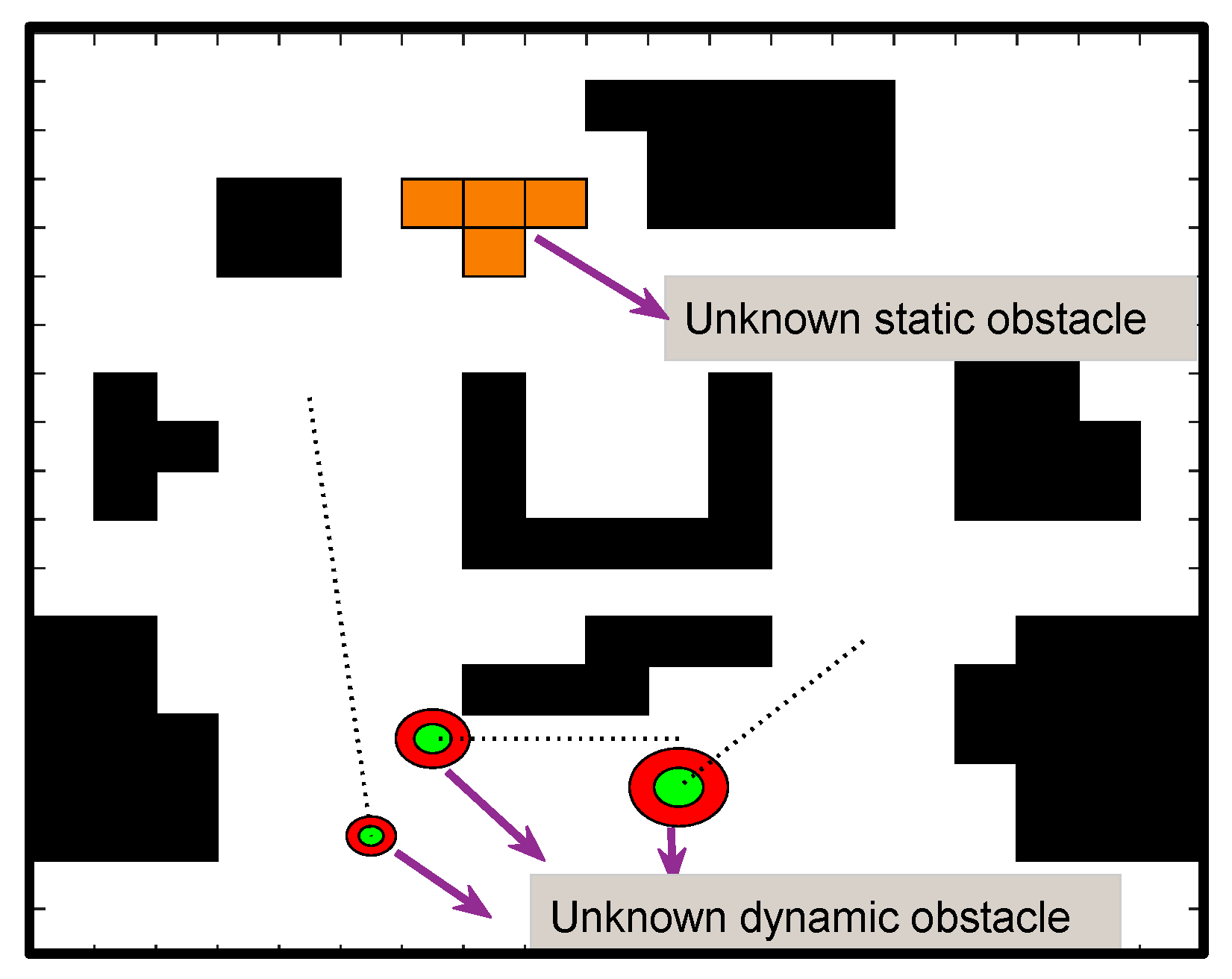
• A new dynamic environment construction method is proposed to address the lack of practical dynamic factors in current path planning research.
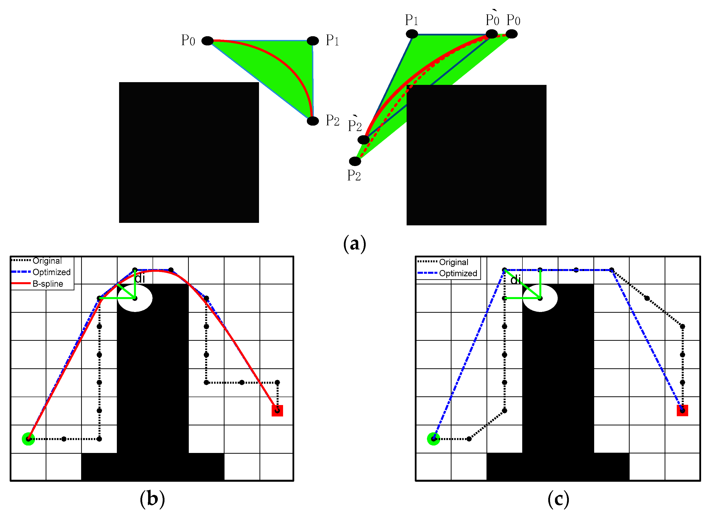
• The robot’s navigation trajectory is planned by the improved ACO, which improves the robot’s adaptability to complex environments in the grid map. We propose a non-uniform initial pheromone method to avoid the blindness of the ants’ initial search and improved heuristic functions using corner suppression factors to enhance the smoothing ability of the ants’ paths of exploration. To improve the algorithm’s convergence, we updated the pheromone hierarchically according to the quality of the ants. In addition, the deadlock problem is solved by the retraction mechanism we designed. Considering the actual path requirements of the robot, we smoothed and optimized the paths.
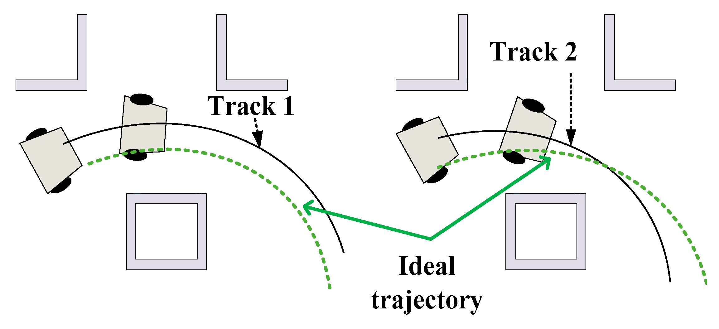
• Constructing the robot model based on improved DWA, our primary focus is to utilize the global path planned by IACO as the robot’s navigation information, then analyze and improve the robot’s sampling window and evaluation function to enhance the path tracking capability, dynamic obstacle avoidance capability, and motion stability. Finally, we have verified the effectiveness of the fusion algorithm through extensive simulation experiments.

2. Environmental Model Construction

Current research on mobile robot path planning is usually based on more ideal environments that lack consideration of certain dynamic environmental factors. This paper proposes a new approach to environment model construction to further extend the research on dynamic path planning.

2.1. Modelling of the Known Environment

A standard method for describing the working environment of a mobile robot is the grid method, which divides the environment into a grid of Mrows and Ncolumns, with the black grids representing the obstacle areas that make the robot impassable and a white grid representing the areas where the robot can pass. Based on the previous ideal environment, this paper will add the dynamic factor environment shown in Figure 1, including unknown static obstacle (the orange grid) and unknown dynamic obstacle (the circular mobile obstacle), after the global path planning process has been implemented.

2.2. Modeling of the Unknown Environment

The robot’s movement is usually disturbed by other unknown obstacles in its environmental space. Better research results on unknown environments focus on unknown static obstacles [7,8]. In contrast, research on unknown dynamic environments [19,24,25] contains problems such as lack of consideration of moving objects’ speed and volume size and unreasonable obstacle avoidance mechanisms in the robots themselves. Considering the above issues, a new dynamic environment modeling requirement is proposed, and a better approach to the robot’s obstacle avoidance strategy will be presented following.

To facilitate the expansion of the volume size of the mobile obstacles, we will consider a circular obstacle instead of a square obstacle [23] limited by the grid method and build a red threat circle with a size of n times the radius $R\_ob$ of the mobile obstacle, which can significantly improve the robot’s recognition area of blocks and enhance obstacle avoidance (we verify with the corresponding experiments). Where: $R\_Sob=nR\_ob$, the absolute velocity vector is $\left(v_{b}cos\theta ,v_{b}sin\theta \right)$, and $\theta$ is the directional angle of the velocity vector $v_b$. The model of the mobile obstacle is shown in Figure 2.

For the ensuing study, we define the mobile robot and its dynamic environment as follows:

(1)

The starting point, endpoint, and global environmental information are known.

(2)

The mobile robot has sensors that can acquire external information and sense the actual volume size and speed of movement of the moving obstacle.

(3)

The mobile robot is based on a two-wheel differential model with the dynamics constraints considered. It has a well-developed power system and sufficient energy to accelerate, decelerate, and avoid obstacles.

(4)

Considering the uncontrollable action of mobile barriers, this paper will focus on the uniform velocity motion and set its movement speed as less than the maximum linear speed of the robot.

(5)

The route of the mobile obstacles motion can be obtained by the security A* algorithm [34], and the dynamic environmental factors are ignored in the planning process. Based on this, we will set the corresponding motion speed for the mobile obstacles and obtain the position information for each moment in advance for the robot to collect data and execute the obstacle avoidance strategy.

3. Global Path Planning

3.1. Ant Colony Optimization (ACO)

Ant colony optimization is an efficient heuristic algorithm that uses distributed computation. The ants choose the direction of movement mainly based on the accumulated pheromones on the path. Assuming that the ant $k$ is located at the node $i$ at time $t$, the probability of selecting the next node $j$ is determined by Equation (1).

$$p_{ij}^k(t)=\{\begin{array}{l}\frac{{[{\tau }_{ij}(t)]}^a{[{\eta }_{ij}\left(t\right)]}^{\beta }}{{\displaystyle \sum _{j\in allowedi}{[{\tau }_{ij}(t)]}^a{[{\eta }_{ij}\left(t\right)]}^{\beta }}},j\in allowedi\hfill \\ 0,otherwise\hfill \end{array}$$

(1)

$${\eta }_{ij}\left(t\right)=1/d_{jE}$$

(2)

where $allowedi$ denotes the set of optional adjacent grids of ant $k$ in grid $i$; ${\tau }_{ij}$ is the pheromone concentration;${\eta }_{ij}$ is the heuristic function and $d_{jE}$ denotes the Euclidean distance from grid $j$ to the endpoint $E$; and $\alpha$ and $\beta$ denote the relative importance degree of ${\tau }_{ij}$ and ${\eta }_{ij},$ respectively. The ant’s search for the optional path is influenced by the pheromone update strategy, which is traditional.

$$\Delta {\tau }_{ij}^k(t)=\{\begin{array}{l}\frac{Q}{L_k},j\in allowedi\\ 0,otherwise\end{array}$$

(3)

$${\tau }_{ij}\left(t+1\right)=\left(1-\rho \right){\tau }_{ij}\left(t\right)+{\displaystyle \sum _{k=1}^m\Delta }{\tau }_{ij}^k\left(t\right)$$

(4)

where $Q$ is the pheromone intensity; $\Delta {\tau }_{ij}^k$ denotes the pheromone increment of the path; $L_k$ denotes the total length of the path traveled by the ant $k; \rho$ is the pheromone volatility factor; and $m$ denotes the total number of ants.

3.2. Improved Ant Colony Optimization (IACO)

3.2.1. Initial Non-Uniform Pheromone

The initial pheromone of the traditional ACO is constant, and the ants tend to move to the grid closer to the endpoint, which may lead the ants in a wrong direction and then continue searching. To improve the quality of the ants’ search paths and to prevent them from falling into dead ends effectively, this paper proposes a method for non-uniformly assigning pheromones based on obstacle density concerning the non-uniform initial pheromone strategy proposed by Luo et al. [12] based on the distance relationship as follows:

$${\tau }_{i,j}(0)=C\cdot f(i)$$

(5)

$$f(i)=card\left(allowedi\right)/8$$

(6)

where $C$ is an amplification factor of the feasibility function, which is taken as needed;$f\left(i\right)$ is the feasibility function; and $card$ indicates the number of feasible neighborhood grids for the grid $i$, with more selectable grids demonstrating greater path feasibility, more pheromones are allocated, and conversely, to a lesser extent. In addition, the pheromone concentration at the map boundary is set to a small constant. Figure 3 shows the initial pheromone concentration of one map, where $C$ is a constant 10 and the boundary pheromone concentration is set to 2, the brighter-colored areas indicate higher pheromone concentrations and more excellent path selectivity.

3.2.2. Design of Heuristic Functions

The traditional heuristic function is shown in Equation (2), which guides the ant to explore the path by the distance relationship from the ant’s current position to the endpoint. The attraction effect becomes more pronounced as the ants get closer to the endpoint. Conversely, the attraction effect is insignificant for parts far from the endpoint. Ant may suffer severe deadlocks and produce more redundant turning points due to the lack of guidance from favorable inspirational information [35]. For this reason, we considered both the heuristic effects of the starting point, the current node, and the endpoint, and then we added a corner suppression factor as shown in Equation (8) to enhance the smoothing ability during ant exploration to reduce redundant nodes. The heuristic function we designed is shown in Equation (7).

$${\eta }_{ij}=\frac{d_{Sj}}{d_{ij}+d_{jE}}\cdot Eturn$$

(7)

$$Eturn=\{\begin{array}{l}{u}_1/Lgrid,turn(J)=turn(J-1)\hfill \\ u_1/\sqrt{2} Lgrid, otherwise \hfill \end{array}$$

(8)

where $d_{Sj}$ is the distance from the starting point $S$ to the next node $j$; $d_{ij}$ is the distance from the current node $i$ to the point $j$; $d_{jE}$ is the distance from the point $j$ to the endpoint $E$; $Eturn$ is the corner suppression factor; $Lgrid$ is the side length of the grid, and we default to 1; $u_1$ is the smoothness weight, taken according to the actual situation; and $turn\left(J\right)$ and $turn\left(J-1\right)$ are the current and previous directions to be transferred by the ant $k$ in the eight-neighborhood range, respectively. The most beneficial effect of our heuristic function is that when $turn\left(J\right)$ is the same as $turn\left(J-1\right)$, it will increase the probability of ant $k$ choosing this path, thus reducing the number of redundant turning points and improving the smoothness of the path. To further demonstrate the effectiveness of the improved initial pheromone strategy and the designed heuristic function, we analyzed it in Section 6.1.1 using first-generation ant populations with no pheromone update disturbance.

3.2.3. Improving Pheromone Updates

Pheromone update refers to accumulation and volatilization, mainly local and global update processes. This paper improves the pheromone update rule by the optimal-worst ant system and the elite ant system. After each round of iteration, we will divide the optimal layer ants, the worst layer ants, and the ordinary layer ants by path length. Then, perform local pheromone updating based on Equations (10)–(12) to increase the role of the optimal solution in guiding and weakening the part of the worst solution. We have also introduced the enhancement factor of the elite ant of Equation (14) into the global pheromone update to speed up the algorithm’s convergence further.

$$\Delta {\tau }_{ij}^k(t)=\{\begin{array}{l}\Delta {\tau }^{best}+\Delta {\tau }^{worst}+\Delta {\tau }^{other},j\in allowedi\hfill \\ 0, otherwise\hfill \end{array}$$

(9)

$$\Delta {\tau }^{best}=\frac{Q_1}{L_{best}},Q_1=bQ$$

(10)

$$\Delta {\tau }^{worst}=\frac{Q_2}{L_{worst}},Q_2=Q/w$$

(11)

$$\Delta {\tau }^{other}=\frac{Q_3}{L},Q_3=Q$$

(12)

where $\Delta {\tau }^{best}, \Delta {\tau }^{worst}, \Delta {\tau }^{other}$ are the local pheromone increments of the optimal, worst and other paths in the current iteration, respectively;$L_{best}, L_{worst}, L$ correspond to the lengths of the three tracks, respectively; $b$ and $w$ are the number of optimal ants and worst ants in the current iteration, respectively; and $Q_1, Q_2, Q_3$ are the pheromone intensity of three types of ants, respectively.

AS the decisions of the ants in the current iteration will be influenced by the previous ants, if the path obtained by the aforementioned method is not optimal, it will mislead the following ants. Therefore, we select elite ants from within $i$ iterations according to Equation (14) and introduce an increase factor in the global pheromone update to amplify the influence of the elite ants, which speeds up the convergence of the algorithm to some extent. The improved global pheromone update is as follows.

$${\tau }_{ij}\left(t+1\right)=\left(1-\rho \right){\tau }_{ij}\left(t\right)+{\displaystyle \sum _{k=1}^m\Delta {\tau }_{ij}^k}\left(t\right)+q\left(t\right)$$

(13)

$$q(t)=\{\begin{array}{l}\delta \frac{N{C}_{\max }}{NC\cdot L^{\ast }(i)},L^{\ast }(i)=min(L)\\ 0,other\end{array}$$

(14)

where $m$ denotes the total number of ants;$\delta$ is the influence value of elite ants; $NC$ and $N{C}_{max}$ are the current and maximum number of iterations, respectively; $min\left(L\right)$ is the optimal path length of the current iteration; and $L^{*}\left(i\right)$ is the path length of the elite ants within $i$ iterations.

3.2.4. Improving the Pheromone Volatility Factor

The optimal-worst ant system and the elite ant system speed up the algorithm’s convergence. To avoid the positive feedback mechanism of the ant colony leading to the optimum local problem, we improve the pheromone volatility factor $\rho$ to enhance the global searchability. If there is no new elite ant, the pheromone volatilization factor is adjusted; otherwise, it is a constant ${\rho }_0$. The improvement strategy is as follows:

$$\rho (t+1)=\{\begin{array}{l}\rho (t)(1+NC/N{C}_{max}),L^{*}(i)=min(L)\\ {\rho }_0,otherwise\end{array}$$

(15)

3.2.5. Deadlock Handling Strategy

When the robot’s environment is complex (e.g., an environment with U-shaped obstacles), the presence of the forbidden table mechanism may lead to a deadlock situation where ants do not have a suitable grid to move. Ant retraction and ant death strategies are common approaches to solving this problem [36]. However, when the environment consists of many or large traps, the ant retraction strategy causes the ants to constantly mark and judge their surroundings, with forwarding and backward situations, resulting in algorithm inefficiency. Similarly, the ant death strategy causes ants with deadlock to die naturally, which means the pheromone is updated inefficiently and poorly in algorithm accuracy.

In this paper, a deadlock measure is proposed based on the ant retreat strategy. As shown in Figure 4, when an ant falls into a deadlocked state at grid D, it is allowed to retreat to the previous path grid T3 and fill the grid D with a virtual obstacle (the blue grid). If the ant is still in a deadlocked state, we continue the backtracking and filling operations until the ant is outside the trap entirely. The beneficial effects of the strategy are (1) ensuring the diversity of the ant colony and improving the adaptability of the algorithm effectively to complex environments and (2) using virtual obstacles to fill in the deadlocked region and then prevent subsequent ants from falling into that part again, improving the algorithm’s solution speed effectively.

3.2.6. Path Smoothing Optimisation

Paths obtained by both the ACO and A* algorithm consist of path nodes in the grid center. The paths, in this case, have more invalid nodes, and the curvature is also discontinuous, which does not satisfy the actual path requirements of the robot. To this, we design a new path smoothing method shown in Figure 5, where the initial path consists of a concatenation of grid centroids, and the original route is a black dashed line with many redundant nodes. We optimize the tracks which no longer limit the grid’s center and take the safety distance $d$ into account, as follows:

• Iterate through all nodes of the path. If the current node is on the same line with two adjacent nodes, the current node is removed;
• Iterate through the starting point and the turning point. From the starting point, each node will be connected to the following turning point as the alternative path in succession and judge the relationship between the distance $di$ of each path to the obstacle grid and the safety distance $d$. If $di\le d$, the alternative path is ignored; if $di>d$ the redundant nodes of the original route are removed to generate this optimized path (the blue dashed line). In this paper, the safety distance $d$ for the paths of the robot and mobile obstacles are 0.707 and 1.414, respectively.
• The three-time B-sample curve has second-order continuity, which can better satisfy the continuity of the mobile robot in terms of velocity and acceleration (the kinetic characteristics are not considered).

  (1)

  Extract the critical nodes as control nodes $P_i\left(i=0,1,\dots ,n\right)$ after removing the redundant nodes.

  (2)

  According to Equation (16), the segmental B-sample smoothing [37] is performed on the turning point to generate the B-sample curve.

  (3)

  To control the B-spline curve to avoid crossing obstacles, Huang et al. [38] adjusted the curve based on the convexity of the curve wrapping. The B-spline curve is retained when the barrier is outside the characteristic triangle formed by the control point $P_i$. Suppose the obstacle intersects the characteristic triangle, and the B-spline curve crosses the obstacle. In that case, a set of triangles with a similarity ratio $k$ is selected within the characteristic triangle ($k$ from 1 to 0, the scale is chosen according to the experiment). This triangle is utilized to generate new control points to determine the shortest B-spline curve that will not cross the obstacle.

  $$C_{0,3}(u)=\frac{1}{6}\left[\begin{array}{cccc}1& u& u^2& u^3\end{array}\right]\left[\begin{array}{cccc}1& 4& 1& 0\\ -3& 0& 3& 0\\ 3& -6& 3& 0\\ -1& 3& -3& 1\end{array}\right]\left[\begin{array}{c}{P}_0\\ P_1\\ P_2\\ P_3\end{array}\right],0\le u\le 1$$

  (16)

Figure 5a is a schematic diagram of control point selection, in which the characteristic triangle consists of control points $\left\{p_0, p_1,p_2\right\}$. There is no collision between the characteristic triangle and the obstacle in the left figure, save the curve. In the right figure, there are collisions, and the measure is to generate new B-sample curves based on control points $\left\{\grave{p_0}, p_1,\grave{p_2}\right\}$ determined by similar triangles until there are no further collisions. Figure 5b is the mobile robot path planning diagram, where IACO planned the black path, the route marked in blue is optimized by steps 1 and 2, and the red trace is obtained by step 3. Figure 5c shows the dynamic obstacle motion path diagram, where the black dashed line is received by the security A* algorithm [34], and the blue dashed line is optimized by steps 1 and 2.

4. Local Path Planning

4.1. Dynamic Window Approach (DWA)

DWA is a local path planning method for predictive control that samples multiple velocities (linear and angular velocities) in the velocity space and simulates the robot’s trajectory at these velocities within a specific time interval. Based on the evaluation metrics, we selected the best speed from multiple sets of simulated trajectories to drive the robot’s motion [19].

4.1.1. Kinematics Model

The two-wheel differential speed model of the mobile robot is shown in Figure 6, where: L is the width of the robot. In the experiment, we can ensure the safety of the robot movement by setting the safety radius $R_{safe}$; $v\left(t\right)$ and $\omega \left(t\right)$ are the linear and angular velocities, respectively. The motion state of the robot during the time interval of the sampling period $\Delta t$ is:

$$\{\begin{array}{l}x(t)=x(t-1)+v(t)\Delta t\cos (\theta (t-1))\hfill \\ y(t)=y(t-1)+v(t)\Delta t\sin (\theta (t-1))\hfill \\ \theta (t)=\theta (t-1)+w(t)\Delta t\hfill \end{array}$$

(17)

where $x\left(t\right), y\left(t\right),\theta \left(t\right)$ denote the position and angle of the robot in the $x,y$ directions at the time $t$, respectively; the linear velocity $v\left(t\right)$ range of variation depends on the nearest distance to the obstacle and the maximum linear deceleration; the content of angular velocity $\omega \left(t\right)$ variation is determined by both the closest distance to the obstruction and the maximum angular deceleration.

4.1.2. Determination of Robot Motion Velocity Range

In the velocity space, DWA describes the robot’s obstacle avoidance problem as an optimization problem with constraints, including incomplete motion constraint on the differential robot, dynamics constraint on the robot structure, and environmental constraints.

(1)

The maximum and minimum speed constraints for the robot are:

$$v_s=\left\{\left(\begin{array}{l}v,w\hfill \end{array}\right)\mid v\in \left[v_{min},v_{max}\right],w\in \left[w_{min},w_{max}\right]\right\}$$

(18)

(2)

Motor acceleration and deceleration constraints: as different motors have different performances, the acceleration of the robotis also different, and the robot is constrained by the speed that can be reached in the nexttime interval.

$$v_d=\{(v,w)\mid v\in \left[v_c-a_v{}^{\min }\Delta t,v_c+a_v{}^{\max }\Delta t\right], w\in \left[w_c-a_w{}^{\min }\Delta t,w_c+a_w{}^{\max }\Delta t\right]\}$$

(19)

where $v_c , w_c$ are the linear velocity and angular velocity of robot at the current moment, respectively; $a_v^{min}, a_w^{min}$ are the minimum linear deceleration and minimum angular deceleration, respectively;$a_v^{max}, a_w^{max}$ are the maximum linear acceleration and maximum angular acceleration, respectively; and $\Delta t$ is the sampling time.

(3)

Braking distance constraint: the entire robot trajectory can be subdivided into several linear or circular motions. To ensure the robot’s safety, the current speed should decelerate to 0 before hitting the obstacle in the maximum deceleration conditions.

$$v_a=\{(v,w)\mid v⩽\sqrt{2dist(v,w)a_v{}^{\min }},w⩽\sqrt{2dist(v,w)a_w{}^{\min }}\}$$

(20)

where $dis\left(v,w\right)$ is the distance between the simulated trajectory and the nearest obstacle. From the expression $0-v_a^2=-2dist\left(v,w\right)a_v^{min}$ and $0-w_a^2=-2dist\left(v,w\right)a_w^{min},$ the simulated velocity must satisfy the condition of Equation (20) to ensure the safety of the robot moves to a greater extent.

The above constraints limit the robot to a certain speed of motion, which we can represent by a velocity set $\left\{V_r\right|V_r=v_s{\displaystyle \cap }{v}_d{\displaystyle \cap }{v}_a\}$.

4.1.3. Evaluation Function

We sampled multiple velocities from the velocity space and then selected the optimal trajectory from them by designing an appropriate evaluation function. The essential criteria are that the robot in local navigation should efficiently avoid obstacles and move quickly and steadily towards the target. The conventional evaluation functions as follows:

$$G(v,w)=\sigma [xheading(v,w)+ydist(v,w)+zvel(v,w)]$$

(21)

where $heading\left(v,w\right)$ is the azimuth evaluation function and to evaluate the azimuth deviation between the end direction of the simulated trajectory and the target at the current speed; $dist\left(v,w\right)$ is the function to evaluate the distance from the trajectory to the obstacle; $vel\left(v,w\right)$ is the current speed magnitude evaluation function; $\sigma$ is the normalization operation, and $x,y,z$ are the weighting factor of each evaluation function.

4.2. Improved Dynamic Window Approach (IDWA)

Conventional DWA lacks global path guidance and is prone to local optimality, for which IACO planned the navigation path. Conventional DWA has good robustness and good obstacle avoidance in static environments, but it may be ineffective when highly moving obstacles arise in the motion space. To enhance the effectiveness of dynamic path planning, the following improvements are made to the evaluation function.

4.2.1. Modifying the $heading\left(v,w\right)$ Function

This function is a navigation function. Considering the situation shown in Figure 7, it is clear that the turning trend of trajectory 1 is more desirable. However, according to the original evaluation function to calculate the angle by the end position of the trajectory, we find $\lambda 1>\lambda 2$, which shows that trajectory 2 has a higher rating than trajectory 1, which is not realistic [39]. In this paper, we changed the navigation target point of the robot after several time intervals on the predicted trajectory we found $\theta 1 < \theta 2$, with trajectory 1 receiving a higher rating.

Most scholars have optimized the global path and extracted key nodes as the navigation points of the robot, but most of them have not considered that the selection of navigation points is not significant if the navigation points are too far from the current position of the robot. In this paper, the heading function is improved according to the robot’s state of motion so that the navigation points are selected concerning the robot’s current position. First, the average distance $\Delta s$ between adjacent path nodes after three B-sample optimizations is calculated by Equation (22), and the desired move-out distance $ds$ is determined, then the navigation point $tar$ is estimated by Equation (24):

$$\Delta s=\frac{length(B\_spline)}{size(B\_spline)}$$

(22)

$$n_{ds}=floor(\frac{ds}{\Delta s})$$

(23)

$$tar=B\_spline(n+n_{ds})$$

(24)

where $length()$ is the path length of the $B\_spline$ curve; $size()$ is the number of nodes for calculating the path;$floor$ is the downward rounding function; $n$ is the sequence of nodes of the current navigation point in the original global path, and the information about the robot’s present moment of navigation point $tar$ is obtained by the expected increase in the number of nodes $n_{ds}$.

As shown in Equation (25), the modified $heading\left(v,w\right)$ function will calculate the deviation angle in terms of the position of the predicted trajectory after several node intervals $n_{ds}$ and give a score accordingly. The robot’s trajectory tracking and navigation capabilities have been improved to a certain extent.

$$headin{g}^{\prime }(v,\omega )={180}^{\circ }-\left|\Theta \left(r,tar\right)-\Theta \left(r\right)\right|$$

(25)

where $\Theta \left(r,tar\right)$ is the predicted angle at which the robot’s position $r$ at the next moment points to the navigation target point $tar$, obtained with its current linear velocity $v$ and angular velocity $\omega$;$\mathrm{and} \Theta \left(r\right)$ is the predicted direction of the robot’s motion.

To ensure the stability of the robot movement and to avoid acceleration and deceleration of the robot wandering between navigation points, the following navigation point $ta{r}^{*}$ information is obtained from Equations (22)–(25) when the robot is moving towards the current navigation point $tar$ and the condition of Equation (26) is satisfied.

$$\begin{array}{ll}ta{r}^{*}=& B\_spline(n+2n_{ds}), dis(r,tar)<d_1\\ & \left|\right|\left[min(dis(r,obs))<d_2\&dis(tar,min\_obs)<d_3\right]\end{array}$$

(26)

where $dis\left(r,tar\right)$ is the distance from the predicted position $r$ to the target point $tar$; $min\left(dis\left(r,obs\right)\right)$ is the shortest distance from the expected position $r$ to the obstacle $obs$ in the robot motion space, and the obstacle is noted as $min\_obs$; $dis\left(tar,min\_obs\right)$ is the distance from the target point $tar$ to the obstacle $min\_obs$; and $d_1, d_2$ and $d_3$ are the reference distances, respectively, and taken as needed.

4.2.2. Modifying the $dist\left(v,\omega \right)$ Function

The function is an obstacle avoidance function. The traditional obstacle list information [40] is shown in Equation (27), including global known obstacles $obs\_closed$ and unknown static obstacles $obs\_static,$ which lacks the consideration of unknown dynamic obstacles $obs\_dynamics\left(t\right)$. For this reason, this paper optimizes the $obs$ to update dynamically over time, as shown in Equation (28):

$$obs=[obs\_closed,obs\_static]$$

(27)

$$obs(t)=[obs(t-1),obs\_dynamics(t)]$$

(28)

Considering the situation shown in Figure 8, it is clear that the trend of obstacle avoidance for trajectory 1 is more desirable. The robot needs to estimate the state information of the mobile obstacle after $\Delta t$ seconds in advance to simulate a path in velocity space that will avoid the obstacle. Based on the line velocity $vo{b}_i \left(i=1,2,\dots ,n\right)$ of the mobile barriers and the current speed $v$ of the robot, we define the prediction time $\Delta t$ as follows:

$$\Delta t=k_{1}int(\frac{v}{vob})+k_2$$

(29)

$$vob=min(vo{b}_1,vo{b}_2,\dots ,vo{b}_n)$$

(30)

where $int$ is an upward rounding function; $k_1, k_2$ are the correction factors, to be taken as required; and $vob$ is the minimum perceived velocity of the mobile obstacle in the robot’s motion space.

The modified $dist\left(v,w\right)$ function will calculate the distance from the current simulated trajectory point to the predicted movement of the moving obstacles after $\Delta t$ time, and discard those trajectories whose shortest distance from the obstacle is less than or equal to the robot’s safety radius $R_{safe}$. In addition, the function has an upper limit on the obstacle distance $D_{max}$, which ignores barriers that are too far from the robot, as shown in Equation (31).

$$dis{t}^{\prime }(v,\omega )=\{\begin{array}{l} min\left[D_{min}\left(r,obs(t+\Delta t)\right),D_{max}\right],D_{min}(r,obs(t+\Delta t))>R_{safe}\\ discarded, D_{min}(r,obs(t+\Delta t))\le R_{safe}\end{array}$$

(31)

where $D_{min}$ is the shortest distance from the robot’s simulated trajectory $r$ to all obstacles, and the calculation of the motion state of all moving obstacles is advanced by $\Delta t$ seconds.

4.2.3. Modifying the $vel\left(v,w\right)$ Function

The function makes the robot move fast, and the score is only related to the robot’s linear velocity. In general, fluctuations in angular momentum tend to cause oscillations, and excessive volatility in angular velocity can affect the stability of the robot’s motion [41]. Considering the situation shown in Figure 9, we assume that the linear speeds of trajectories 1 and 2 are the same. Trajectory 1 has a more uniform angular variation and a more desirable turning trend. Referring to the heuristic function improvement of IACO in this paper, the speed score and $vel\left(v,w\right)$ function are improved as follows:

$$p=\{\begin{array}{l}{u}_2, \omega 1\le \left|({\omega }_{t-2}-{\omega }_{t-1})-({\omega }_{t-1}-{\omega }_t)\right|\le \omega 2\\ u_2/\sqrt{2}, otherwise\end{array}$$

(32)

$$velocit{y}^{\prime }(v,\omega )=v+p$$

(33)

where $P$ is the angular velocity score; ${\omega }_{t-2}, {\omega }_{t-1}$ and ${\omega }_t$ are the angular velocity of the robot at the first two moments, first one moment and the current moment, respectively; and $u_2,\omega 1$ and $\omega 2$ are the correction factor.

5. Hybrid Path Planning

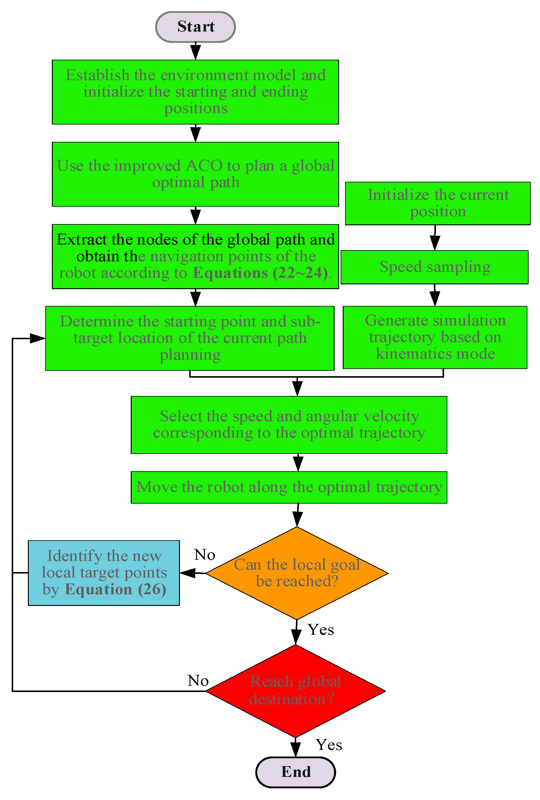
In this paper, ACO and DWA are fused to obtain the robot’s global navigation path using IACO and construct a robot’s kinematic model for dynamic path planning using IDWA. The basic process of the hybrid path planning method is as follows:

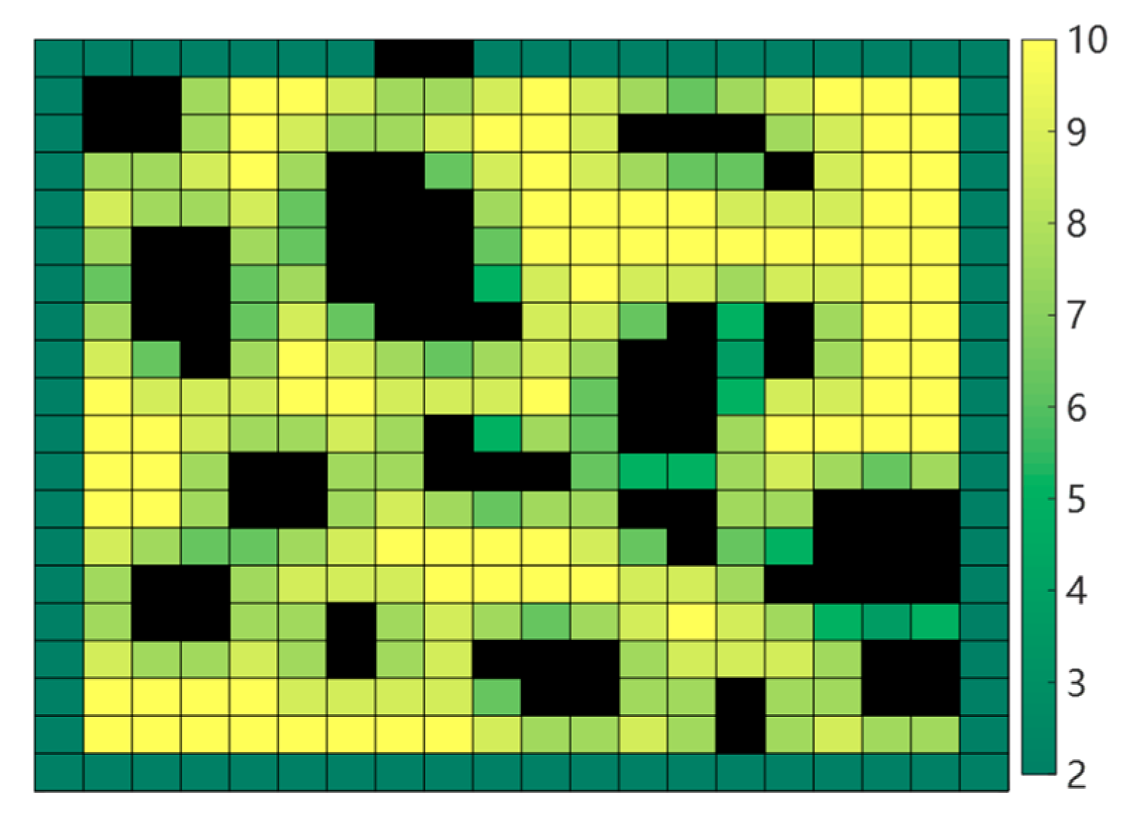
Step 1. Build a grid map for the mobile robot.

Step 2. Plan a global path based on the IACO with smoothing optimization.

Step 3. Extract the nodes of the global path and obtain the navigation points of the robot according to Equations (22)–(24). The distance and azimuth angle from the current position to the local target will be calculated in the IDWA.

Step 4. When the robot moves towards the position of the local target point, once a new obstacle appears in the environment and is within the detection range of the robot, the information (position, volume size, and speed of movement) will be sensed by the robot and the corresponding strategy will be executed to avoid the obstacle.

Step 5. When the robot approaches the local target point, or a new obstacle appears on the original path that prevents the robot from approaching the local target point, a new target point will be reacquired according to Equation (26).

Step 6. The path planning and movement process will stop when the mobile robot reaches the global target point or when the global target point is unreachable due to obstacles occupying.

A flow chart of the hybrid path planning algorithm is shown as Figure 10:

6. Simulation Experimental Analysis

This paper uses Matlab 2016a software to conduct experiments on a Windows 10 computer with a 2.2 GHz processor and 8 GB of RAM.

6.1. Performance Analysis of the IACO

6.1.1. Initial Population Validity Analysis

We propose an initial pheromone approach considering smoothness and a heuristic function with a corner suppression factor, making the paths be fewer turning points and higher smoothness in a natural environment. To exemplify the effects of population diversity and path smoothing, we conduct experimental analyses in a conventional environment through the first generation of ant colonies without pheromone update disturbances. The number of ants is 50; the initial pheromone concentration of the traditional ACO is 10; the initial pheromone concentration in this paper is assigned according to Equations (5) and (6), with C set to 20 and the pheromone concentration on the boundary set to 2. The experimental results are shown in

Table 1. Initial population algorithm performance comparison table.

Evaluation Criteria	Traditional ACO	This Paper
Average path length /m	47.9479	42.9443
Worst path length /m	82.0760	64.8660
Optimal path length /m	32.0380	32.1400
Number of turns for optimal path	12	4
Number of ants dead	15	0
Optimal search time /s	0.3287	0.1822

and Figure 11 and Figure 12.

The experimental simulation results show that the first generation of traditional ACO finds paths based on heuristic functions under the same conditions of pheromone concentration, resulting in more concentrated paths with poor population diversity, which is not conducive to the exploration ability of the algorithm. In this paper, IACO has a better guiding effect on the first generation of ants, and the distribution of ants in the whole space is more uniform. The population diversity is better, which is more likely to guide the subsequent ants to achieve the globally optimal path. From Table 1, we can see that our initial population pathfinding effectiveness is significantly better than the traditional ACO. In subsequent experiments, we will utilize the improved pheromone update strategy to further demonstrate our algorithm’s effectiveness in solving the contradictory population diversity and convergence speed.

6.1.2. Analysis of the Effectiveness of Deadlock Solutions

To verify the effectiveness of the deadlock problem-solving strategies in this paper, the traditional ant-death strategy and the retraction strategy are chosen to conduct comparative experiments in a specific large-scale deadlock map environment. After extensive experiments in this environment, the following parameters are selected for the retraction and death strategies, respectively: $\alpha =1, \beta =7, \rho =0.7,Q=10,m=50$; $\alpha =1,\beta =15,\rho =0.9,Q=10,m=50$. The parameters in this paper are shown in

Table 2. Main parameters of the simulation experiment.

Algorithm	$\mathit{\alpha }$	$\mathit{\beta }$	$\mathit{Q}$	$\mathit{\rho }$	$\mathit{c}$	${\mathit{u}}_1$	$\mathit{\delta }$
Traditional ACO	1	10	100	0.3	-	-	-
Luo et al. [12]	1.1	7	100	0.2	-	-	-
Dai et al. [13]	1	10	50	0.3	-	-	-
You et al. [14]	1	2	1	0.2	-	-	-
This paper	1	7	10	0.7	20	1	10

. The path and iteration diagram of all ants are added to reflect the level of pathfinding for different strategies, and the results of the simulation experiments are shown in

Table 3. Performance comparison table of algorithms for deadlock environment.

Evaluation Criteria	Retraction Strategy	Death Strategy	This Paper
Length of path/m	125.1840	37.2100	32.7260
Number of turns for optimal path	25	19	3
Number of iterations	——	13	5
Number of ant deaths before the algorithm reaches convergence	0	108	0
Optimal search time /s	24.5955	2.4646	1.3852

and Figure 13, Figure 14 and Figure 15.

The simulation results show that the retraction strategy preserves all the ants’ solutions. Still, the ants move forward and backward repeatedly in the deadlocked region, leaving a large amount of interference pheromone for subsequent ants. The pathfinding ability of ants becomes worse and worse as the iteration progresses, showing that the retraction strategy is not suitable for the large-scale trap environment. Although the death strategy is more effective than the retraction strategy in terms of path length and iteration, the number of ants that died due to deadlock before the algorithm achieved convergence is as high as 35.8%, negatively impacting the ability to solve the optimal solution. The death strategy can achieve better paths than the retraction strategy, but it is trapped in a local optimum and cannot be improved by changing the pheromone volatility factor anymore. This paper enhances the algorithm based on the advantage of the retraction strategy, which can preserve ants’ survival and improve the solution effect. From the experimental results, the ants in this paper retreat from the deadlocked region in time and add a virtual barrier grid to the deadlocked area to prevent subsequent ants from falling into this part, which improves the path search quality of the following ants. Our strategy can obtain better paths in large-scale deadlock environments, and the search time is also shorter, which is more suitable for path planning of mobile robots in a complex environment.

6.2. Simulation Experiment Analysis of IACO

A general environment of 20 × 20 scale and a U-shaped environment are chosen for comparison experiments, with a population of 50 ants and the number of iterations set to 50.

6.2.1. General Environment

To verify the effectiveness and superiority of our IACO, the traditional ACO, algorithms from Luo et al. [12], and Dai et al. [13] are selected for comparative experimental analysis in a conventional environment that is based on Luo et al. [12]. The results of the simulation experiments are shown in

Table 4. General environment algorithm performance comparison table.

Evaluation Criteria	This Paper			Luo et al. [12]	Dai et al. [13]	Traditional ACO
	Original	Optimized	Spline
Path length/m	33.3137	33.0226	32.1817	30.9680	34.4840	30.9680
Number of turns for optimal path	7	7	0	15	8	15
Number of iterations	3	——	——	6	9	28
Optimal search time /s	1.772	0.603	0.380	1.816	1.619	2.084

and Figure 16, where: the black dashed line in Figure 16a is the initial path of our algorithm, the blue dashed line is the path after optimizing the redundant nodes, and the solid red line is the path of three times B-sample smoothing; the paths in Figure 16b marked with black, purple and blue are implemented by Dai et al. [13], Luo et al. [12], and traditional ACO, respectively.

As shown in Figure 16, both the traditional ACO and the Luo et al. [12] can find the shortest path of 30.9690 m, where the Luo et al. [12] algorithm converges faster, and the number of turns for both is 15, which is more than this paper and Dai et al. [13]. Too many turns for the mobile robot will inevitably consume more energy and time. In this paper and Dai et al. [13], the path length and smoothing factors are considered as the objective of the search, where the length and the number of turning points of the initial path obtained by our algorithm are 33.3137 m and 7, respectively, which are slightly better than the 34.4840 m and 8 of Dai et al. [13]. The B-spline curve is obtained by optimizing the initial path with 2.3023 m shorter than Dai et al. [13], and it is significantly better than the other three algorithms in terms of smoothness and curvature continuity suitable for the robot. We consider hierarchical optimization for our pheromone update strategy, so the convergence of our algorithm is the fastest, as can be seen in Figure 16c. The downside is that as we consider the optimization path twice, the total program run time is 2.755 s, slightly more than others.

6.2.2. U-Shaped Environment

To verify the effectiveness and superiority of our algorithm in a U-shaped environment, the traditional ACO, Dai et al. [13], and You et al. [14] algorithms are chosen for comparative experimental analysis, with the map environment based on You et al. [14]. The results of the simulation experiments are shown in

Table 5. Performance comparison table for U-shaped environment algorithms.

Evaluation Criteria	This Paper			Dai et al. [13]	You et al. [14]	Traditional ACO
	Original	Optimized	B_Spline
Path length/m	28.6274	28.1842	27.9103	29.2100	28.6557	29.4520
Number of turns for optimal path	4	4	0	5	7	8
Number of iterations	6	——	——	23	12	22
Optimal search time /s	1.494	0.543	0.255	1.299	1.355	2.047

and Figure 17, where: the blue grid in Figure 17a is the virtual obstacle grid used to handle the deadlock strategy in this paper; the paths in Figure 17b are marked with black, purple and blue are implemented by Dai et al. [13], You et al. [14], and traditional ACO, respectively.

From Figure 17, we can see that some ants in the pathfinding process of traditional ACO in the deadlocked region have a death situation, making the optimal path is caught in the local optimum. The algorithm in this paper obtains the optimal path in the current environment, which is slightly better than the algorithms of Dai et al. [13], and You et al. [14] in terms of path length, where: our initial path length is 28.6274 m, 28.1842 m after removing redundant nodes, and the final B-sample curve is 27.9103 m, which is 4.4% and 2.6% reduced compared to the path length of Dai [13] et al. and You [14] et al., respectively. More importantly, the initial path planned by our algorithm has only four turns, which is better than the algorithms of Dai et al. [13], and You et al. [14] with five and seven turns, respectively. At a particular time cost, the quality of our paths is much better after two smoothing operations. In addition, we perform a hierarchical optimization of the pheromone update, and as seen in Figure 17c, our algorithm converges in the 6th generation, outperforming other algorithms.

6.3. Experimental Analysis of the IACO-IDWA

To validate the performance of our improved ACO fusion improved DWA, the A* fusion DWA algorithm [7], which is currently widely studied for hybrid path planning, is chosen for experimental analysis of algorithm comparison in unknown static and unknown dynamic environments. Chi et al. [7] use the improved A* to plan global paths with a high degree of safety (maintaining a safe distance from obstacles), combined with the traditional DWA for local path planning. The standard parameters of our DWA and the DWA of Chi et al. [7] are: the maximum velocity is $1 \mathrm{m}/\mathrm{s}$; the maximum angular velocity is ${20}^{\mathrm{o}}/\mathrm{s}$; the velocity resolution is $0.01 \mathrm{m}/\mathrm{s}$; the angular velocity resolution is $1^{\mathrm{o}}/\mathrm{s}$; the acceleration is $0.2 \mathrm{m}/{\mathrm{s}}^2$; the angular acceleration is ${50}^{\mathrm{o}}/{\mathrm{s}}^2$; the parameters of the evaluation function are: $x=0.1,y=0.05,z=0.2$; the prediction period is 3s; the safety radius $R_{safe}$= 0.7 m; the desired displacement distance $ds$ is 5m; the navigation point reference distance $d_1, d_2$ and $d_3$ are 2m; the prediction time (moving obstacle) parameter: $k_1$ is 10, $k_2$ is 0; and the angular velocity scoring parameter: $u_2$ is 0.1 $,\omega 1$ is 0, and $\omega 2$ is 0.1 rad.

6.3.1. Unknown Static Obstacle Environments

Our algorithm is compared with Chi et al. [7], and the results are shown in Figure 18, Figure 19 and Figure 20 and

Table 6. IACO- IDWA path planning performance table.

Number of Unknown Static Obstacles	Path Length/m		Optimal Search Time/s
	Chi et al. [7]	This Paper	Chi et al. [7]	This Paper
1	36.6681	35.8240	402.3918	409.8574
2	37.1823	36.1200	419.0973	417.4700
3	37.7814	36.5060	447.5673	422.6949

. In this case, the black dotted line represents the global path of each algorithm, where the original path length planned by Chi et al. [7] is 36.5210 m, and this paper is 35.4772 m. After the global path planning is completed, we add unknown static obstacles to the common part of the path, where: the paths marked with blue and purple represent local paths of Chi et al. [7] and our algorithm, respectively.

In Simulation Experiment 1, when a random obstacle is added to the map, both Chi et al. [7] and our algorithm can plan a path from the starting point (top left corner) to the target point (bottom right corner). The actual path length of the robot driving in this paper is 35.8240m, which is 2.2% optimized compared to Chi et al. [7]. As the initial path of Chi et al. [7] maintains a safe distance from the obstacles and reduces the constraints of barriers on the robot pathfinding space, the algorithm takes lesser time than our algorithm. As shown in Table 6, the robot still could avoid the obstacles better and more safely to reach the target point by increasing the number of random obstacles, with the driving path length also growing, but the path length of our algorithm is always better than Chi et al. [7].

In Simulation Experiments 2 and 3, the algorithm of Chi et al. [7] has more seek time than our algorithm as the new random obstacle is placed at a more critical location on the global path, then the robot is influenced by the more enormous spatial constraints of the environment. The DWA used in Chi et al. [7] is based on the turning point of the global path as the key navigation point, and when the navigation point is less helpful in guiding the robot, it is costly for the robot to search for a path that can bypass this obstacle. Therefore, in Figure 19c and Figure 20c, we can observe that the movement speed of the robot in Chi et al. [7] varies dramatically and more persistently than our robot between 200–300 and 400–600 control nodes. The algorithm in this paper calculates the deviation angle with the desired trajectory node position by a modified $heading\left(v,w\right)$ function, which is not limited to the traditional DWA that only considers the path turning point case. Moreover, in this paper, when the robot moves towards the current navigation point and satisfies the condition of Equation (26), the following navigation point is obtained in advance, which avoids the acceleration and deceleration situation where the robot wanders between local target points, and the stability of robot motion more than Chi et al. [7]. In summary, the hybrid algorithm in this paper can achieve obstacle avoidance in an unknown environment and better fit the globally optimal path.

6.3.2. Unknown Dynamic Obstacle Environments

In the previous section, we verified the effect of the hybrid path planning of the improved algorithm. Still, due to the difference in the path planned by the global algorithm, the obstacle avoidance effect of our algorithm cannot be fully explained. Therefore, in this section, we verify the dynamic obstacle avoidance effect of the algorithm by a mobile obstacle in the 10 × 10 obstacle-free environment. Consider three types of moving blocks with different characteristics (size, speed), as shown in

Table 7. Mobile obstacle movement states.

Simulation Experiment	$\mathbf{Actual} \mathbf{Radius} \mathit{R}\_\mathit{o}\mathit{b} /\mathbf{m}$	$\mathbf{Radius} \mathit{R}\_\mathit{S}\mathit{o}\mathit{b}$$\mathbf{of} \mathbf{Threat} \mathbf{Circle}$	Speed of Movement of m/s
1	0.15	0.3	0.1
2	0.3	0.6	0.1
3	0.3	0.6	0.4

. In the experiment, the actual radius of the mobile obstacle is extended twice to generate a threat circle which expanded threat circle can increase the robot’s recognition range of barriers and play a certain degree of buffering effect on the robot’s braking. The start point coordinates of the mobile robot are (3.5, 7.5), and the endpoint coordinates are (6.5, 2.5). The start point coordinates of the mobile obstacle are (6.5, 4.5), and the endpoint coordinates are (3.5, 6.5).

To facilitate the study, we modify the obstacle list of the function in Chi et al. [7] to be dynamic through Equation (28). Usually, most scholars study DWA in a way similar to Chi et al. [7], that is, for the detection distance $D_{min}$ in Equation (31) taken as the distance from the robot to the geometric center of the obstacle. A reasonable safety radius $R_{safe}$ is set for the robot, so the predicted trajectory will not consider those areas where the detection distance is less than the safety radius $R_{safe}.$ Considering the limited space for robot movement, if the volume of mobile obstacles is too large, a more effective safety radius $R_{safe}$ needs to be chosen to ensure the simulated trajectory process, for which we improved it and added a set of experiments based on Chi et al. [7]. The detection distance considered in the improved algorithm [7] and this paper will be the distance from the robot to the surface of the obstacle threat circle.

The mobile obstacle in Simulation Experiment 1 is considered smaller in size and lower in motion speed. From

Table 8. Performance analysis of IACO-IDWA for path planning.

Simulation Experiment		Chi et al. [7]	Improved Algorithm [7]	This Paper
1	Length of the robot’s driving path/m	5.8415	5.9656	6.0727
	Optimal search time /s	73.3436	89.7258	81.2701
2	Length of the robot’s driving path/m	5.8415	6.0905	6.2377
	Optimal search time /s	106.3393	125.5351	76.1026
3	Length of the robot’s driving path/m	5.9284	6.4851	7.0157
	Optimal search time /s	82.5480	99.0592	124.8771

and Figure 21, we can see that all three methods avoid the obstacles, and the robot also travels a similar path length, with the algorithm in Chi et al. [7] taking the least time to avoid the obstacle. In Simulation Experiment 2, the volume size of the moving obstacle is double that of Experiment 1, and the robot in Chi et al. [7] collides with the threat circle shown in Figure 22a, but after improving the obstacle detection method of Chi et al. [7], its can successfully avoid the obstacle safely. The algorithm in this paper predicts the motion of the moving block for $\Delta t$ periods and pre-avoids the obstacle at position (4, 6.2), with better safety in obstacle avoidance than the improved algorithm [7]. Simulation Experiment 3 further increased the speed of obstacle motion to 0.4 m/s. From Figure 23, we can see that in a dynamic environment with a larger volume and more enormous motion speed mobile obstacle, the robot in Chi et al. [7] collided with it, and the improvement crossed the threat circle, nearly colliding with the mobile obstacle. The theoretical maximum linear velocity of 1 m/s that we set for the robot is not achieved due to the robot receiving motion constraints, dynamics constraints, and obstacle constraints. Hence, our robot successfully searched for a path to avoid the obstacle at the cost of time for path search. From the above experiments, it is clear that our algorithm is suitable for a wide range of dynamic environments, and the following experiments will validate the algorithm in more complex dynamic environments.

6.3.3. Complex Dynamic Environments

The above experiments have verified the effectiveness of IACO global path planning and the obstacle avoidance capability of IDWA. This simulation further demonstrates the dynamic obstacle avoidance feasibility of the fusion algorithm in complex environments by setting up different levels of unknown complex environments, illustrated by a simulation example below.

In this example, firstly, a static environment for the robot is established in a 40 × 40 grid environment, and the optimal global path with a path length of 55.5667m from the starting point (1.5, 40.5) to the endpoint (40.5, 1.5) is planned based on IACO, as shown by the black dashed line in Figure 24. Next, setting unknown dynamic obstacles in this environment, the robot moves along the global path, judges the surrounding environment in real-time, and avoids obstacles according to their conditions. The experimental results are shown in

Table 9. Comparison table of robot paths.

		Path Length/m	Number of Robot Control Nodes	Optimal Search Time/s
Static path planning		55.5667	——	2.2415
Dynamic path planning	Simulation Experiment 1	56.2028	1206	357.1979
	Simulation Experiment 2	56.6224	1215	417.6458
	Simulation Experiment 3	57.3136	1228	437.0259
	Simulation Experiment 4	58.4793	1248	524.4448

and Figure 24, Figure 25 and Figure 26, and due to the difference in computer performance, the algorithm running time does not represent the actual robot movement time. In this case, the number of control nodes of the robot represents its motion time, and every ten nodes simulate 1s in natural environments.

In Simulation Experiment 1, the robot performs real-time path planning along the global path, and the path is essentially the same as the original. Once again, IDWA’s track tracking capability is proven. The robot passed safely under this path without colliding any obstacles, and the final path length is 56.2028 m, taking 120.6 s.

Simulation Experiment 2 is based on Experiment 1. We set up a mobile obstacle with an actual radius $R\_ob$ of 0.3 m, a threat circle $R\_Sob$ of 0.6 m, and an unknown static block. We designed the mobile barrier to move in opposite directions to the robot, where: the starting point coordinates are (10.5, 33.5); the endpoint coordinates are (3.5, 38.5); the movement speed is 0.16 m/s; and the trajectory is marked in black dashed. At the moment of process 1, the robot finds the mobile obstacle moving towards itself with a speed of 0.16 m/s through the sensor, executes the obstacle avoidance strategy, and completes the obstacle avoidance at the moment of process 2. An unknown static obstacle is sensed at position (14.5, 29.5) during the movement towards the local target point, and the obstacle avoidance strategy is executed again. By the improved $heading\left(v,w\right)$ function, the robot eventually moves to the endpoint, and the final path length is 56.6224 m, taking 121.5 s.

Simulation Experiment 3 added a further mobile obstacle 2 with an actual radius $R\_ob$ of 0.2 m and a threat circle radius $R\_Sob$ of 0.4 m and larger volumes of unknown static obstacles to Experiment 2. We designed the mobile obstacle 2 to move in the same direction as the robot, where: the starting coordinates are (7.5, 34.5), the ending coordinates are (15.5, 27.5), and the speed of movement is 0.08 m/s. After avoiding the mobile obstacle 1, the robot detects a mobile obstacle 2 ahead occupying the original path at a rate of 0.08 m/s and again executes the obstacle avoidance strategy and overtakes it at the moment of process 3. The unknown static obstacles are sensed at position (25, 20), which occupies the robot’s path, and the robot executes the obstacle avoidance strategy until the end. The final path length is 57.3136 m, and the time taken is 122.8 s.

Simulation Experiment 4 further builds on Experiment 3 by adding two mobile obstacles and several unknown static obstacles, where: mobile obstacle 3 has an actual radius $R\_ob$ of 0.4 m and a threat circle radius $R\_Sob$ of 0.8 m, and we designed it to come from the side of the robot with starting coordinates of (39.5, 18.5) and ending coordinates of (16.5, 25.5), moving at a speed of 0.288 m/s; the actual radius $R\_ob$ of mobile obstacle 4 is 0.375 m and a threat circle radius $R\_Sob$ of 0.75 m, and we design it in the robot’s global path, with the starting point coordinates are (38.5, 13.5) and the ending point coordinates are (34.5, 9.5), moving at a speed of movement is 0.09 m/s. After avoiding mobile obstacle 1 and mobile obstacle 2, the robot detects a mobile obstacle 3 coming towards itself at 0.288 m/s on its side at process 4 and executes an obstacle avoidance strategy to avoid it after process 5 and 6 successfully. During the local exploration process, mobile obstacle 4 is detected to have stopped moving, and the robot treated it as an unknown static obstacle to avoid and eventually moved safely to the end position. The final path length is 58.4793 m, and the time taken is 124.8 s.

The changes in linear velocity, angular velocity, and attitude angle of the robot in the Simulation Experiment 4 have been recorded in Figure 25. We can see that the robot’s motion is generally stable after improving the evaluation function, and it can maintain a uniform speed throughout the motion, and the change of angular velocity is relatively smooth.

7. Conclusions and Future Work

This paper investigates a new hybrid algorithm for dynamic path planning in view of the ant colony algorithm’s excellent robustness and search capability and the dynamic window approach’s local obstacle avoidance advantages. To further refine the dynamic factors of the robot in the natural environment, a new dynamic environment construction method is proposed. The robot obtains a global reference trajectory based on an improved ant colony algorithm in unknown territory and uses mounted sensors to gain information about the strange environment for dynamic obstacle avoidance.

We are taking into account the poor adaptability of traditional ACO to complex environments and the difference between the path and the actual requirements of the robot. We propose a non-uniform initial pheromone method to avoid the blindness of the ant’s initial search. Then, the smoothing heuristic function with corner suppression and the improved retraction strategy is used to optimize the ant’s ability to explore paths in complex environments. To address the inefficiencies of the ACO, pheromones are updated in layers. Moreover, we present a path smoothing method to satisfy the motion requirements of the robot better in a grid environment.

Considering the poor navigation capability and poor dynamic obstacle avoidance capability of the traditional DWA, we construct the robot model with kinematic constraints using IDWA and utilize the global path planned by IACO as the robot’s navigation information. Then we improve the sampling window and evaluation function, which eventually enhances the robot’s path tracking capability, dynamic obstacle avoidance capability, and motion stability. The experiment shows that the proposed method enables the robot to efficiently and safely navigate in global static environments and better dynamic obstacle avoidance in complex dynamic environments.

In this paper, the robot is kinematically constrained, but this is neglected when planning global paths, and we will consider it in path planning and path smoothing processes in the subsequent studies. Moreover, the dynamic environment considered in this paper is limited to a two-dimensional environment, and it is hoped that our proposed approach will be of some use to subsequent researchers in studying three-dimensional dynamic environments.

References

1. Pandey, A.; Parhi, D.R. Optimum path planning of mobile robot in unknown static and dynamic environments using Fuzzy-Wind Driven Optimization algorithm. Def. Technol. 2017, 13, 47–58. [Google Scholar] [CrossRef]
2. Pandini, M.M.; Spacek, A.D.; Neto, J.M.; Ando, O.H. Design of a didatic workbench of industrial automation systems for engineering education. IEEE Lat. Am. Trans. 2017, 15, 1384–1391. [Google Scholar] [CrossRef]
3. Sidoti, D.; Avvari, G.V.; Mishra, M.; Zhang, L.; Nadella, B.K.; Peak, J.E.; Hansen, J.A.; Pattipati, K.R. A multiobjective path-planning algorithm with time windows for asset routing in a dynamic weather-impacted environment. IEEE Trans. Syst. Man Cybern. Syst. 2016, 47, 3256–3271. [Google Scholar] [CrossRef]
4. Roy, D.; Chowdhury, A.; Maitra, M.; Bhattacharya, S. Geometric Region-Based Swarm Robotics Path Planning in an Unknown Occluded Environment. IEEE Trans. Ind. Electron. 2020, 68, 6053–6063. [Google Scholar] [CrossRef]
5. Josef, S.; Degani, A. Deep Reinforcement Learning for Safe Local Planning of a Ground Vehicle in Unknown Rough Terrain. IEEE Robot. Autom. Lett. 2020, 5, 6748–6755. [Google Scholar] [CrossRef]
6. Montiel, O.; Orozco-Rosas, U.; Sepúlveda, R. Path planning for mobile robots using Bacterial Potential Field for avoiding static and dynamic obstacles. Expert Syst. Appl. 2015, 42, 5177–5191. [Google Scholar] [CrossRef]
7. Chi, X.; Li, H.; Fei, J.Y. Research on random obstacle avoidance method for robots based on the fusion of improved A~* algorithm and dynamic window method. Chin. J. Sci. Instrum. 2021, 42, 132–140. [Google Scholar] [CrossRef]
8. Qi, J.; Yang, H.; Sun, H. MOD-RRT*: A sampling-based algorithm for robot path planning in dynamic environment. IEEE Trans. Ind. Electron. 2020, 68, 7244–7251. [Google Scholar] [CrossRef]
9. Sivaranjani, S.; Nandesh, D.A.; Raja, R.K.; Gayathri, K.; Ramanathan, R. An Investigation of Bug Algorithms for Mobile Robot Navigation and Obstacle Avoidance in Two-Dimensional Unknown Static Environments. In Proceedings of the 2021 International Conference on Communication information and Computing Technology (ICCICT), Mumbai, India, 25–27 June 2021; pp. 1–6. [Google Scholar] [CrossRef]
10. Lee, D.H.; Lee, S.S.; Ahn, C.K.; Shi, P.; Lim, C.-C. Finite Distribution Estimation-based Dynamic Window Approach to Reliable Obstacle Avoidance of Mobile Robot. IEEE Trans. Ind. Electron. 2021, 68, 9998–10006. [Google Scholar] [CrossRef]
11. Yang, L.; Fu, L.; Li, P.; Mao, J.; Guo, N.; Du, L. LF-ACO: An effective formation path planning for multi-mobile robot. Math. Biosci. Eng. 2022, 19, 225–252. [Google Scholar] [CrossRef] [PubMed]
12. Luo, Q.; Wang, H.; Zheng, Y.; He, J. Research on path planning of mobile robot based on improved ant colony algorithm. Neural Comput. Appl. 2020, 32, 1555–1566. [Google Scholar] [CrossRef]
13. Dai, X.; Long, S.; Zhang, Z.; Gong, D.W. Mobile robot path planning based on ant colony algorithm with A* heuristic method. Front. Neurorobotics 2019, 13, 15. [Google Scholar] [CrossRef] [PubMed]
14. You, X.; Liu, S.; Zhang, C. An improved ant colony system algorithm for robot path planning and performance analysis. Int. J. Robot. Autom. 2018, 33, 527–533. [Google Scholar] [CrossRef] [Green Version]
15. Xu, K.; Lu, H.; Huang, Y.; Hu, S.J. Robot path planning based on double-layer ant colony optimization algorithm and dynamic environment. Acta Electonica Sin. 2019, 47, 2166. [Google Scholar] [CrossRef]
16. Ao, B.Q.; Yang, S.; Ye, Z.H. Improved ant colony algorithm for unmanned surface vehicle smooth path planning. Control. Theory Appl. 2021, 38, 1006–1014. [Google Scholar] [CrossRef]
17. Lazarowska, A. Discrete artificial potential field approach to mobile robot path planning. IFAC-PapersOnLine 2019, 52, 277–282. [Google Scholar] [CrossRef]
18. Zhong, X.; Tian, J.; Hu, H.; Peng, X.F. Hybrid Path Planning Based on Safe A* Algorithm and Adaptive Window Approach for Mobile Robot in Large-Scale Dynamic Environment. J. Intell. Robot. Syst. 2020, 99, 65–77. [Google Scholar] [CrossRef]
19. Yuan, X.; Yuan, X.; Wang, X. Path Planning for Mobile Robot Basedon Improved Bat Algorithm. Sensors 2021, 21, 4389. [Google Scholar] [CrossRef]
20. Chen, T.J.; Sun, Y.; Dai, W.; Tao, W.; Liu, S. On the Shortest and Conflict-Free Path Planning of Multi-AGV System Based on Dijkstra Algorithm and the Dynamic Time-Window Method. Adv. Mater. Res. 2013, 645, 267–271. [Google Scholar] [CrossRef]
21. Zhang, H.; Zhang, C.; Yang, W.; Chen, C.-Y. Localization and navigation using QR code for mobile robot in indoor environment. In Proceedings of the IEEE International Conference on Robotics & Biomimetics, Zhuhai, China, 6–9 December 2015; pp. 2501–2506. [Google Scholar] [CrossRef]
22. Liu, L.-S.; Lin, J.-F.; Yao, J.-X.; He, D.-W.; Zheng, J.-S.; Huang, J.; Shi, P. Path Planning for Smart Car Based on Dijkstra Algorithm and Dynamic Window Approach. Wirel. Commun. Mob. Comput. 2021, 2021, 1–12. [Google Scholar] [CrossRef]
23. Shao, L.; Li, Q.; Li, C.; Sun, W.T. Mobile Robot Path Planning Based on Improved Ant Colony Fusion Dynamic Window Approach. In Proceedings of the 2021 IEEE International Conference on Mechatronics and Automation (ICMA), Takamatsu, Japan, 8–11 August 2021; pp. 1100–1105. [Google Scholar] [CrossRef]
24. Jin, Q.; Tang, C.; Cai, W. Research on Dynamic Path Planning Based on the Fusion Algorithm of Improved Ant Colony Optimization and Dynamic Window Method. IEEE Access 2021. [Google Scholar] [CrossRef]
25. Zhang, X.; Chen, X. Path Planning Method for Unmanned Surface Vehicle Based on RRT* and DWA. In Proceedings of the International Conference on Multimedia Technology and Enhanced Learning, Virtual Event, 8–9 April 2021; pp. 518–527. [Google Scholar] [CrossRef]
26. Chen, Y.-W.; Chiu, W.-Y. Optimal robot path planning system by using a neural network-based approach. In Proceedings of the 2015 International Automatic Control Conference (CACS), Yilan, Taiwan, 18–20 November 2015; pp. 85–90. [Google Scholar] [CrossRef]
27. Wu, P.; Cao, Y.; He, Y.Q.; Li, D.C. Vision-based robot path planning with deep learning. In International Conference on Computer Vision Systems; Springer: Cham, Switzerland, 2017; pp. 101–111. [Google Scholar] [CrossRef]
28. Wu, Q.; Zhang, Y.; Guo, K.; Wang, X. LSTM combined with reinforcement learning dynamic environment path planning algorithm. J. Chin. Comput. Syst. 2021, 42, 334–339. [Google Scholar] [CrossRef]
29. Mnih, V.; Kavukcuoglu, K.; Silver, D.; Graves, A.; Antonoglou, L.; Wierstra, D.; Riedmiller, M. Playing atari with deep reinforcement learning. arXiv 2013, arXiv:1312.5602. [Google Scholar]
30. Mirowski, P.; Pascanu, R.; Viola, F.; Soyer, H.; Ballard, A.J.; Banino, A.; Denil, M.; Goroshin, R.; Sifre, L.; Kavukcuoglu, K.; et al. Learning to navigate in complex environments. arXiv 2016, arXiv:1611.03673. [Google Scholar]
31. Panov, A.I.; Yakovlev, K.S.; Suvorov, R. Grid path planning with deep reinforcement learning: Preliminary results. Procedia Comput. Sci. 2018, 123, 347–353. [Google Scholar] [CrossRef]
32. Lei, X.; Zhang, Z.; Dong, P. Dynamic path planning of unknown environment based on deep reinforcement learning. J. Robot. 2018, 2018, 1–10. [Google Scholar] [CrossRef]
33. Lv, L.; Zhang, S.; Ding, D.; Wang, Y.X. Path planning via an improved DQN-based learning policy. IEEE Access 2019, 7, 67319–67330. [Google Scholar] [CrossRef]
34. Chen, R.N.; Wen, C.C.; Peng, L.; You, C.Z. Application of improved A~* algorithm in robot indoor path planning. Comput. Appl. 2019, 39, 1006–1011. [Google Scholar] [CrossRef]
35. Wu, X.; Wei, G.; Song, Y.; Huang, X. Improved ACO-based path planning with rollback and death strategies. Syst. Sci. Control. Eng. 2018, 6, 102–107. [Google Scholar] [CrossRef] [Green Version]
36. Zhang, H.; He, L.; Yuan, L.; Ran, T. Path planning for mobile robots based on improved two-layer ant colony algorithm. Control. Decis. Mak. 2021, 1–10. [Google Scholar] [CrossRef]
37. Yang, H.; Qi, J.; Miao, Y.; Sun, H.; Li, J. A New Robot Navigation Algorithm Based on a Double-Layer Ant Algorithm and Trajectory Optimization. IEEE Trans. Ind. Electron. 2019, 66, 8557–8566. [Google Scholar] [CrossRef] [Green Version]
38. Huang, D.J.; Lei, X.; Jiang, C.F.; Chen, Y.M.; Ding, Y.D. Global path planning for film group animation based on improved JPS algorithm. J. Shanghai Univ. Nat. Sci. Ed. 2018, 24, 694–702. [Google Scholar] [CrossRef]
39. Chang, L.; Shan, L.; Dai, Y.W.; Qi, Z.D. Improved DWA-based multi-robot formation control in unknown environments. Control. Decis. Mak. 2021, 1–10. [Google Scholar] [CrossRef]
40. Liu, Z.; Liu, H.; Lu, Z.; Zeng, Q. A Dynamic Fusion Pathfinding Algorithm Using Delaunay Triangulation and Improved A-Star for Mobile Robots. IEEE Access 2021, 9, 20602–20621. [Google Scholar] [CrossRef]
41. Chang, L.; Shan, L.; Jiang, C.; Dai, Y.W. Reinforcement based mobile robot path planning with improved dynamic window approac h in unknown environment. Auton. Robot. 2021, 45, 51–76. [Google Scholar] [CrossRef]
Figure 1. The natural working environment of the robot.
Machines 10 00050 g001
Figure 2. Mobile obstacle.
Machines 10 00050 g002
Figure 3. Diagram of initial pheromone allocation.
Machines 10 00050 g003
Figure 4. Deadlock handling strategy diagram; (a) Ant deadlock diagram; (b) Improved fallback strategy.
Machines 10 00050 g004
Figure 5. Schematic diagram of path smoothing optimisation; (a) Editable node determination; (b) The path of mobile robot; and (c) The path of mobile obstacle.
Machines 10 00050 g005
Figure 6. Robot kinematics model.
Machines 10 00050 g006
Figure 7. h e a d i n g ( v , w ) mechanistic analysis.
Machines 10 00050 g007
Figure 8. d i s t ( v , ω ) mechanistic analysis.
Machines 10 00050 g008
Figure 9. v e l ( v , w ) mechanistic analysis.
Machines 10 00050 g009
Figure 10. Flowchart of the hybrid algorithm.
Machines 10 00050 g010
Figure 11. Diagram of the optimal path of ACO; (a) Optimal path diagram; (b) All ants’ paths diagram.
Machines 10 00050 g011
Figure 12. Diagram of the optimal path of this paper; (a) Optimal path diagram; (b) All ants’ paths diagram.
Machines 10 00050 g012
Figure 13. Retraction strategy optimisation path diagram; (a) Optimal path diagram; (b) All ants’ paths diagram; (c) Iterative diagram of the optimal path; and (d) Iterative diagram of ants’ paths.
Machines 10 00050 g013
Figure 14. Death Strategy Optimisation Path Diagram; (a) Optimal path diagram; (b) All ants’ paths diagram; (c) Iterative diagram of the optimal path; and (d) Iterative diagram of ants’ paths.
Machines 10 00050 g014
Figure 15. Diagram of the optimal path of this paper; (a) Optimal path diagram; (b) All ants’ paths diagram; (c) Iterative diagram of the optimal path; and (d) Iterative diagram of ants’ paths.
Machines 10 00050 g015
Figure 16. Comparison diagram of path planning; (a) Optimal path diagram of this paper; (b) Optimal path diagrams of other algorithms; and (c) Optimal path iteration diagram.
Machines 10 00050 g016
Figure 17. Comparison diagram of path planning; (a) Optimal path diagram of this paper; (b) Optimal path diagrams of other algorithms; and (c) Optimal path iteration diagram.
Machines 10 00050 g017
Figure 18. Comparison of path planning results for unknown static environment 1; (a) Local path planning [7] (b) This paper; and (c) Line speed comparison diagram.
Machines 10 00050 g018
Figure 19. Comparison of path planning results for unknown static environment 2; (a) Local path planning [7] (b) This paper; and (c) Line speed comparison diagram.
Machines 10 00050 g019
Figure 20. Comparison of path planning results for unknown static environment 3; (a) Local path planning [7] (b) This paper; and (c) Line speed comparison diagram.
Machines 10 00050 g020
Figure 21. Comparison of path planning results for unknown dynamic environment 1; (a) Chi et al. [7]; (b) Improved algorithm [7]; and (c) This paper.
Machines 10 00050 g021
Figure 22. Comparison of path planning results for unknown dynamic environment 2; (a) Chi et al. [7]; (b) Improved algorithm [7]; and (c) This paper.
Machines 10 00050 g022
Figure 23. Comparison of path planning results for unknown dynamic environment 3; (a) Chi et al. [7]; (b) Improved algorithm [7]; and (c) This paper.
Machines 10 00050 g023
Figure 24. Global optimal path of the robot.
Machines 10 00050 g024
Figure 25. Variation of robot motion parameters in a dynamic environment 4; (a) Diagram of the robot’s linear and angular velocity variation; (b) Diagram of the robot’s angular variation.
Machines 10 00050 g025
Figure 26. Robot path planning process in a dynamic environment; (a) Simulation Experiment 1; (b) Simulation Experiment 2; (c) Simulation Experiment 3; and (d) Simulation Experiment 4.
Machines 10 00050 g026aMachines 10 00050 g026b