
A CNN-Based Method for Counting Grains within a Panicle

School of Mechanical Engineering, Shanghai Jiao Tong University, Shanghai 200240, China
*
Author to whom correspondence should be addressed.
Machines 2022, 10(1), 30; https://doi.org/10.3390/machines10010030
Submission received: 15 November 2021
/
Revised: 18 December 2021
/
Accepted: 19 December 2021
/
Published: 1 January 2022
(This article belongs to the Special Issue Recent Advances in Computer Vision Technology and Its Agricultural Application)
Abstract
:The number of grains within a panicle is an important index for rice breeding. Counting manually is laborious and time-consuming and hardly meets the requirement of rapid breeding. It is necessary to develop an image-based method for automatic counting. However, general image processing methods cannot effectively extract the features of grains within a panicle, resulting in a large deviation. The convolutional neural network (CNN) is a powerful tool to analyze complex images and has been applied to many image-related problems in recent years. In order to count the number of grains in images both efficiently and accurately, this paper applied a CNN-based method to detecting grains. Then, the grains can be easily counted by locating the connected domains. The final error is within 5%, which confirms the feasibility of CNN-based method for counting grains within a panicle.
1. Introduction
With the global population growth, the demand for high-yield crop is increasing [1]. Rice, as the most common food, has become the research object of many researchers. Generally, genotype and phenotype are combined to study rice cultivation [2,3], and how to calculate the yield is one of the core questions. Phenotypic studies usually include traits such as leaves, grains, spikes, etc. [4] Grains’ number within a panicle can directly reflect the yield. Manual phenotypic analysis is a time-consuming and laborious task. Studies show that introducing computer vision technology to the field of phenotypic analysis can greatly increase plant productivity [5]. To meet the needs of automation in phenotypic research [6,7,8], methods of image pattern recognition, such as image segmentation based on the OTSU algorithm and GA (Genetic Algorithm) [9], is applied to the grain counting, which can also be used to get the number of internodes and primary branches. However, the result is not accurate, due to the excessive image patterns of the grains.
In recent years, many intelligent algorithms have started to be applied in agriculture [10,11,12]. The approach that has achieved many remarkable results in the field of agricultural image processing is deep learning [13]. The convolutional neural network (CNN) is one of the main methods of deep learning in the field of computer vision [14]. CNN is widely used for tasks such as image recognition [15], target detection [16], image segmentation [17], and image reconstruction [18], and performs better than traditional methods or even humans in many fields [19]. This is mainly because CNN can effectively extract the features of images [20,21], and some improved CNN structures perform well in target detecting [22,23,24]. A deep neural network has better capability of mining the features of an image with respect to the general neural network. It is suitable for establishing nonlinear and complex mapping relationship. However, the disadvantage is the explosive growth of parameters, especially in image processing. CNN is such a kind of deep neural network designed to reduce the number of parameters, but it maintains the ability to extract complex features of images. A typical CNN structure is (LeNet5) [25].
CNN mainly consists of three kinds of layers: the convolution layer, the pooling layer, and the fully connected layer. The convolution layer is the core part of CNN, using the convolution kernel to share parameters [26]. The size of a convolution kernel is generally no larger than 7 × 7, and the number of convolution kernels depends on that of channels of input and output in each layer. The pooling layer further reduces the number of parameters [27]. Generally, the maximum or average pooling method is adopted. The fully connected layer is the same as that in traditional neural network, which connects each “pixel” in the input map with that in output map, playing a role of integration.
Because CNN has a strong feature extraction capability, it is possible to use CNN for grain counting. There are precedents for using CNN for the segmentation and counting of granular objects. In 2015, Olaf Ronneberger used U-Net to segment a variety of biological cell microscopic images, and the IOU of the segmentation results were all above 70%, which was significantly improved compared to the suboptimal algorithm [28]. Reza Moradi Rad used U-Net to count and centroid the human embryonic cells (blastomeres), which has an average accuracy of 88.2% for embryos of –one to five cells [29]. Jian Chen used U-Net to segment and count aphids on plant leaves, achieving an accuracy of 95.63% and a recall rate of 96.50% [30]. Thorsten Falk developed a suite of software for cell detection, segmentation, counting, and morphometry using U-Net and 3D U-Net for easy use by more researchers [31]. J. Luo proposed an Expectation Maximization (EM)-like self-training method that makes it possible to train U-Net cell counting networks with a small number of samples [32]. Yue Guo combines U-Net and the Self-Attention module to propose a new network structure SAU-Net, which reduces the generalization gap for small datasets [33]. Sambuddha Ghosal designed a deep learning framework for sorghum head detection and counting, which is based on weakly supervised method [34]. However, until now, no scholar has applied U-Net to count grains within a panicle.
This article is aimed at the grain count problem. The method of sample labeling was designed. The software of sample labeling was developed. The appropriate sample expansion method was proposed. Based on numerous panicle image samples, a method of labeling and a fully convolutional network [35] based on U-Net were designed to achieve the goal of detecting grains within a panicle. The appropriate loss function was selected to train the model. Combining with the method of detecting the connected domain, the counting of grains within a panicle was finally realized. Finally, the counting effect was evaluated. The results show that the error of this algorithm was within 5%.
2. Samples Generation
2.1. Image Acquisition Instrument
In order to perform genotypic–phenotypic analysis on rice, our laboratory has designed a seed and panicle phenotyping instrument, as shown in Figure 1. The main modules of this platform include a tablet computer, electronic weighing module, embedded Bluetooth control module, top light board, backlight board, transparent tray, box, etc. This instrument can perform wind selection, weighing, and imaging on seeds and panicles. The panicle samples are taken from the rice RIL (recombinant inbred lines) population in this study, which was derived by single-seed descents from a cross between Oryza sativa ssp. Indica variety JP69 and Oryza sativa ssp. japonica variety Jiaoyuan5A, which show high yield heterosis in hybridized combination and are widely planted in Shanghai, China. All plants were planted in a paddy field in Minhang (31.03° N, 121.45° E), Shanghai, during the summer seasons in 2017–2020. The experimental design was a randomized complete block design (including one row of each inbred line and eight plants in each row).
The main function of the phenotyping instrument in this article is to collect images. The related internal structure is shown in Figure 2. When collecting images, the whole earhead is fixed by several magnetic pressers, and the camera of the tablet computer is facing the center hole of the top light board to complete the image acquisition.
2.2. Image Annotation and Preprocessing
As the number of grains within a panicle is large, the accuracy will be low if the grains’ number is directly selected as the output of the network. A better way is to transform this counting problem into semantic segmentation and connected region counting, realized by CNN, of which the input is the original image and the output is a binary image. The pixels of grains are marked as 1, and the remaining pixels are marked as 0. It is difficult to separate some connected regions when two or more grains are stuck together if the outline of the grain is marked. Therefore, this paper used spots to mark the grains’ locations, and this process is supported by a specific software developed in this paper. It is important that, if a grain is severely blocked, it will not be labeled. The diameter of the spot is 16 pixels.
Figure 3 shows the interface of the marking program. The left button can be clicked to mark the location of a grain, and the right button can be clicked to delete the mark. The final result is as shown in Figure 4.
The size of the original panicle image is 3264 × 2448, and it is reduced by a ratio of 0.77. Then, it is cut into many 160 × 160 (pixels) blocks. Generally, a block contains 10 or fewer grains. Random rotation, flip, and scaling are applied to the original samples to enrich the samples. The range of random rotating angle is from 0 to 360 degrees, and the proportion of random scaling is from 0.8 to 1.2.
More than 80% of the region in a panicle image is background. A distribution unbalance of effective and ineffective samples will arise if training samples are directly generated by a sliding window, which affects the speed and accuracy of the training process. Thus, the ratio of the number of images containing grains to that of pure background is controlled to about 5:1, as shown in Figure 5. The sixth image contains no grain, marked as pure background.
This paper has taken 120 pictures of panicles, of which 80 are chosen as the parents of the training set. After processing, more than 40,000 samples were generated.
3. Design of Neural Network
The input of the network is a RGB image, and the output is a probability image of single channel. The value of each pixel represents the probability of whether the location belongs to the center of the grain. The size of output image is in accordance with that of the input image. The overall structure is shown in Figure 6.
This network consists of the input, nine convolution cells (from C1 to C9), and the output. Each rectangle represents a set of feature maps. The height of the rectangle stands for the size of feature maps. The width stands for the number of channels. The input is a RGB image, having three channels. The output is an image of probability, only having one channel. C1, C2, …and C9 are complex convolution cells, each containing two convolution layers, and the sizes of convolution kernels are all 3 × 3. The number of convolution kernels depends on the channels of feature maps. The blue arrows represent the pooling layers, of which the sizes are all 2 × 2, and the number of channels remains the same after the pooling process. The green arrows represent the up-sampling layers, using the interpolation algorithm to double the size of feature maps. The grey arrows represent the copying and merging process, which reduces the loss of original information caused by up-sampling. The activation functions are all Rectified Linear Units (ReLUs), except the last layer, of which the activation function is the sigmoid function. The size of the input image is marked as H × H, where H should be greater than 48 and divided by 16. The number of channels in C1 is K, and the remaining parameters are as shown in Table 1.
The loss function is similar to the crossing entropy loss function. For each pixel p,
where represents the label (1 or 0) and represents the output of network (floating-point number, from 0 to 1). In this paper, the positive samples refer to the center region of the grains, which means the positive samples are much fewer than the negative samples. To reduce the influence of this unbalance, a coefficient is necessary. In this paper, is taken as 5, which is equivalent to supplementing the positive samples.
The overall loss function, L, is the sum of the loss of each pixel (Euclidean distance) in each batch of images. N represents the number of a batch of images. M represents the number of pixels in an image.
In this paper, the Jaccard Similarity Coefficient (IoU) is used to evaluate the convergence of the network.
where represents the labeling image, and represents the output image processed by a threshold of 0.5. The operator means the multiplication of pixels at the same location. To avoid the denominator being 0, .
4. Training Process
To compare the influence of different sizes of input image and number of channels on the prediction accuracy and testing speed, four groups of parameters are selected to train the networks. (H, K) are, respectively, selected as (48, 10), (80, 16), (112, 24), and (160, 32). A total of 36,000 samples were selected as the training set and the remaining 4000 as the validation set. The number of training samples per batch was 32. The total number of training iterations was 10,000.
As shown in Figure 7, at the beginning, especially the first 2000 steps, the IoU rises faster and then converges. The network reaches the optimal convergence state. In addition, the larger H of the input image, the higher the obtained IoU.
Table 2 compares the occupied size of the models with different training parameters.
5. Result
A sliding window is used to intercept the image and evaluate it. The actual input of the network is a sub region of the original image. The boundary error may rise due to the lack of information from neighboring pixel. In this paper, image splicing is carried out by the way of boundary overlap. In the stitching process, the sliding step is slightly smaller than the length of the clipping image.
The boundary trimming offset is set to u pixels, and the width of overlapping region is set to v pixels. The sliding step(Sub) in sampling process is
The sliding step(Step) in stitching process is
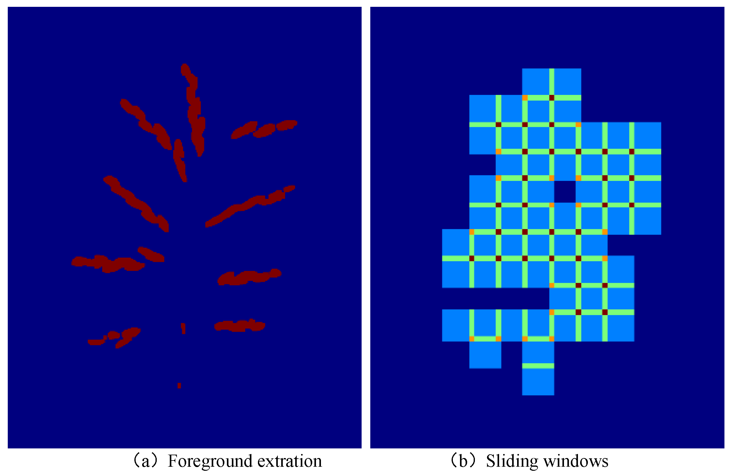
Most pixels in one image belong to the background. If the sliding window skips the region that does not contain grains, it will reduce much computation. In this paper, the color space was conversed from RGB to the HSV, followed by segmentation in the S channel. Then, the small debris was removed by operating morphological opening. The background was filtered based on the obtained foreground. As shown in Figure 8, the foreground was clipped. This method reduces the amount of calculation by 70%.
The result of the grain counting algorithm can be visualized by Figure 9.
6. Analysis
In this paper, four networks with different parameters are tested, and three evaluation criteria are compared.
Mean absolute error (MAE) is a conventional measure of absolute error, which is robust to outliers, as shown in Equation (6):
Mean squared error (MSE) is an important indicator for regression problems, which is more sensitive to outliers than MAE:
Mean relative error (MRE) is dimensionless and usually used to measure the relative error
where represents the predicted grain number, represents the actual grain number, and represents the number of test samples.
Figure 10 shows the result under different parameters. The blue points represent the actual value, and the red points represent the predicted value. The abscissa represents the image index, and the ordinate represents the grain number.
The performance comparison of models with different parameters is shown in Rows 1 to 4 of Table 4. Generally speaking, the larger H and K, the higher the accuracy. However, all of these four networks obtain high accuracies. All the MAEs are lower than 5.0%, which meets most requirements. The fourth network can be applied to a device with high performance, and the first network can be applied to a mobile device. Model 1 is chosen to be deployed on the Xiaomi Tablet 2 of our phenotype instrument, which took 4.6 s to process an entire image of rice panicle.
The performance comparison between the proposed model and classical algorithms such as wavelet [36] and P-trap [37] is shown in Rows 5 to 6 of Table 4. From the results, it can be seen that the method proposed in this paper shows lower MAE and MRE than the wavelet method, and the model with parameters H = 160 and K = 32 outperforms the wavelet method in terms of MSE metrics. The model we proposed also outperforms the P-trap method with respect to MAE, MSE, and MRE. Meanwhile, the computational time is logged to show the real-time performance of different algorithms. Typically, the processing times of different algorithms are evaluated on the platform of 2.0 GHz Intel Core Duo CPU, 2.0 G RAM, MATLAB environment, and WIN10 OS, which shows the computational workloads of the deep neural-network-based models are comparable to those of analytic models in their real-time performance. Since all the CNN-based models are fast enough, even for large size batch samples, the precision factor dominates the final practice of applications, and hereby, Model 4 with 89.8 M memory occupation and 264.90 ms computation time is the optional pre-installed software for the instrument. In conclusion, the method proposed in this paper has better performance than the classical method.
7. Conclusions
In this paper, a marking method for the grain counting within a panicle is designed based on the features of a panicle image, and a convolution neural network is designed and trained. In the prediction stage, the acceleration technique based on the foreground extraction is proposed, and different parameters are compared. The final MAEs are all lower than 5.0%, overcoming the difficulty of counting grains within a panicle.
Author Contributions
Conceptualization L.G., methodology, L.G. and S.F.; software, S.F.; validation, L.G. and S.F.; formal analysis, L.G. and S.F.; investigation, L.G. and S.F.; resources, L.G.; data curation, L.G. and S.F.; writing—original draft preparation, L.G. and S.F.; writing—review and editing, L.G. and S.F.; visualization, S.F.; supervision, L.G.; project administration, L.G.; funding acquisition, L.G. All authors have read and agreed to the published version of the manuscript.
Funding
This work was supported by the Project of UK Royal Society Challenge-led Project/Global Challenge Research Fund (CHL\R1\180496).
Institutional Review Board Statement
Not applicable.
Informed Consent Statement
Not applicable.
Data Availability Statement
Not applicable.
Acknowledgments
The authors will thank Zhihong Ma and Wei Wu for their involvement in conceptualization of this paper.
Conflicts of Interest
The authors declare no conflict of interests.
References
- Zhang, Q.F. Strategies for developing green super rice. Proc. Natl. Acad. Sci. USA 2007, 104, 16402–16409. [Google Scholar] [CrossRef] [Green Version]
- Han, B. Genome-Wide Assocation Studies (GWAS) in Crops. In Proceedings of the Plant and Animal Genome Conference (PAG XXIV), San Diego, CA, USA, 10–15 January 2014. [Google Scholar]
- Zhu, Z.H.; Zhang, F.; Hu, H.; Bakshi, A.; Robinson, M.R.; Powell, J.E.; Montgomery, G.W.; Goddard, M.E.; Wray, N.R.; Visscher, P.M.; et al. Integration of summary data from GWAS and eQTL studies predicts complex trait gene targets. Nat. Genet. 2016, 48, 481–487. [Google Scholar] [CrossRef] [PubMed]
- Xing, Y.Z.; Zhang, Q.F. Genetic and Molecular Bases of Rice Yield. Annu. Rev. Plant Biol. 2010, 61, 421–442. [Google Scholar] [CrossRef] [PubMed]
- Mochida, K.; Koda, S.; Inoue, K.; Hirayama, T.; Tanaka, S.; Nishii, R.; Melgani, F. Computer vision-based phenotyping for improvement of plant productivity: A machine learning perspective. Gigascience 2019, 8, giy153. [Google Scholar] [CrossRef] [Green Version]
- Reuzeau, C. TraitMill (TM): A high throughput functional genomics platform for the phenotypic analysis of cereals. In Vitro Cell. Dev. Biol. Anim. 2007, 43, S4. [Google Scholar]
- Neumann, K. Using Automated High-Throughput Phenotyping using the LemnaTec Imaging Platform to Visualize and Quantify Stress Influence in Barley. In Proceedings of the International Plant & Animal Genome Conference XXI, San Diego, CA, USA, 12–16 January 2013. [Google Scholar]
- Golzarian, M.R.; Frick, R.A.; Rajendran, K.; Berger, B.; Roy, S.; Tester, M.; Lun, D.S. Accurate inference of shoot biomass from high-throughput images of cereal plants. Plant Methods 2011, 7, 2. [Google Scholar] [CrossRef] [PubMed] [Green Version]
- Hao, H.; Chun-bao, H. Research on Image Segmentation Based on OTSU Algorithm and GA. J. Liaoning Univ. Technol. 2016, 36, 99–102. [Google Scholar]
- Huang, P.; Zhu, L.; Zhang, Z.; Yang, C. Row End Detection and Headland Turning Control for an Autonomous Banana-Picking Robot. Machines 2021, 9, 103. [Google Scholar] [CrossRef]
- Cao, X.; Yan, H.; Huang, Z.; Ai, S.; Xu, Y.; Fu, R.; Zou, X. A Multi-Objective Particle Swarm Optimization for Trajectory Planning of Fruit Picking Manipulator. Agronomy 2021, 11, 2286. [Google Scholar] [CrossRef]
- Wu, F.; Duan, J.; Chen, S.; Ye, Y.; Ai, P.; Yang, Z. Multi-Target Recognition of Bananas and Automatic Positioning for the Inflorescence Axis Cutting Point. Front. Plant Sci. 2021, 12, 705021. [Google Scholar] [CrossRef] [PubMed]
- Greenspan, H.; Ginneken, B.v.; Summers, R.M. Guest Editorial Deep Learning in Medical Imaging: Overview and Future Promise of an Exciting New Technique. IEEE Trans. Med. Imaging 2016, 35, 1153–1159. [Google Scholar] [CrossRef]
- Voulodimos, A.; Doulamis, N.; Doulamis, A.; Protopapadakis, E. Deep Learning for Computer Vision: A Brief Review. Comput. Intell. Neurosci. 2018. [Google Scholar] [CrossRef]
- He, K.M.; Zhang, X.; Ren, S.; Sun, J. Deep Residual Learning for Image Recognition. In Proceedings of the 2016 IEEE Conference on Computer Vision and Pattern Recognition (Cvpr), Las Vegas, NV, USA, 27–30 June 2016; pp. 770–778. [Google Scholar]
- Redmon, J.; Divvala, S.; Girshick, R.; Farhadi, A. You Only Look Once: Unified, Real-Time Object Detection. In Proceedings of the 2016 IEEE Conference on Computer Vision and Pattern Recognition (Cvpr), Las Vegas, NV, USA, 27–30 June 2016; pp. 779–788. [Google Scholar]
- Wu, H.; Zhang, J.; Huang, K.; Liang, K.; Yu, Y. FastFCN: Rethinking Dilated Convolution in the Backbone for Semantic Segmentation. arXiv 2019, arXiv:1903.11816. [Google Scholar]
- Gupta, H.; Jin, K.H.; Nguyen, H.Q.; McCann, M.T.; Unser, M. CNN-Based Projected Gradient Descent for Consistent CT Image Reconstruction. IEEE Trans. Med. Imaging 2018, 37, 1440–1453. [Google Scholar] [CrossRef] [PubMed] [Green Version]
- Chen, L.; Wang, S.; Fan, W.; Sun, J.; Naoi, S. Beyond Human Recognition: A CNN-Based Framework for Handwritten Character Recognition. In Proceedings of the 3rd Iapr Asian Conference on Pattern Recognition Acpr, Kuala Lumpur, Malaysia, 3–6 November 2015; pp. 695–699. [Google Scholar]
- Jingying, Q.; Xian, S.; Xin, G. Remote sensing image target recognition based on CNN. Foreign Electron. Meas. Technol. 2016, 8, 45–50. [Google Scholar]
- Yunju, J.; Ansari, I.; Shim, J.; Lee, J. A Car Plate Area Detection System Using Deep Convolution Neural Network. J. Korea Multimed. Soc. 2017, 20, 1166–1174. [Google Scholar]
- Girshick, R. Fast R-CNN. In Proceedings of the 2015 IEEE International Conference on Computer Vision (Iccv), Santiago, Chile, 7–13 December 2015; pp. 1440–1448. [Google Scholar]
- Ren, S.Q.; He, K.; Girshick, R.; Sun, J. Faster R-CNN: Towards Real-Time Object Detection with Region Proposal Networks. IEEE Trans. Pattern Anal. Mach. Intell. 2017, 39, 1137–1149. [Google Scholar] [CrossRef] [PubMed] [Green Version]
- He, K.M.; Gkioxari, G.; Dollár, P.; Girshick, R. Mask R-CNN. In Proceedings of the 2017 IEEE International Conference on Computer Vision (Iccv), Venice, Italy, 22–29 October 2017; pp. 2980–2988. [Google Scholar]
- Lecun, Y.; Bottou, L.; Bengio, Y.; Haffner, P. Gradient-based learning applied to document recognition. Proc. IEEE 1998, 86, 2278–2324. [Google Scholar] [CrossRef] [Green Version]
- Dumoulin, V.; Visin, F. A guide to convolution arithmetic for deep learning. arXiv 2016, arXiv:1603.07285. [Google Scholar]
- Scherer, D.; Muller, A.; Behnke, S. Evaluation of Pooling Operations in Convolutional Architectures for Object Recognition. Artif. Neural Netw. 2010, 6354 Pt III, 92–101. [Google Scholar]
- Ronneberger, O.; Fischer, P.; Brox, T. U-Net: Convolutional Networks for Biomedical Image Segmentation. Med. Image Comput. Comput. Assist. Interv. 2015, 9351, 234–241. [Google Scholar]
- Rad, R.M.; Saeedi, P.; Au, J.; Havelock, J. Blastomere Cell Counting and Centroid Localization in Microscopic Images of Human Embryo. In Proceedings of the 2018 IEEE 20th International Workshop on Multimedia Signal Processing (MMSP), Vancouver, BC, Canada, 29–31 August 2018. [Google Scholar]
- Chen, J.; Fan, Y.; Wang, T.; Zhang, C.; Qiu, Z.; He, Y. Automatic Segmentation and Counting of Aphid Nymphs on Leaves Using Convolutional Neural Networks. Agronomy 2018, 8, 129. [Google Scholar] [CrossRef] [Green Version]
- Falk, T.; Mai, D.; Bensch, R.; Çiçek, Ö.; Abdulkadir, A.; Marrakchi, Y.; Böhm, A.; Deubner, J.; Jäckel, Z.; Seiwald, K.; et al. U-Net: Deep learning for cell counting, detection, and morphometry. Nat. Methods 2019, 16, 67–70. [Google Scholar] [CrossRef]
- Luo, J.; Oore, S.; Hollensen, P.; Fine, A.; Trappenberg, T. Self-training for Cell Segmentation and Counting. Adv. Artif. Intell. 2019, 11489, 406–412. [Google Scholar]
- Guo, Y.; Stein, J.; Wu, G.; Krishnamurthy, A. SAU-Net: A Universal Deep Network for Cell Counting. In Proceedings of the 10th ACM International Conference on Bioinformatics, Computational Biology and Health Informatics, Niagara Falls, NY, USA, 7–10 September 2019; ACM: New York, NY, USA, 2019; pp. 299–306. [Google Scholar]
- Ghosal, S.; Zheng, B.; Chapman, S.C.; Potgieter, A.B.; Jordan, D.R.; Wang, X.; Singh, A.K.; Singh, A.; Hirafuji, M.; Ninomiya, S.; et al. A Weakly Supervised Deep Learning Framework for Sorghum Head Detection and Counting. Plant Phenomics 2019, 2019, 14. [Google Scholar] [CrossRef] [PubMed] [Green Version]
- Shelhamer, E.; Long, J.; Darrell, T. Fully Convolutional Networks for Semantic Segmentation. IEEE Trans. Pattern Anal. Mach. Intell. 2017, 39, 640–651. [Google Scholar] [CrossRef]
- Gong, L.; Lin, K.; Wang, T.; Liu, C.; Yuan, Z.; Zhang, D.; Hong, J. Image-based on-panicle rice [Oryza sativa L.] grain counting with a prior edge wavelet correction model. Agronomy 2018, 8, 91. [Google Scholar] [CrossRef] [Green Version]
- Faroq, A.T.; Adam, H.; Dos Anjos, A.; Lorieux, M.; Larmande, P.; Ghesquière, A.; Jouannic, S.; Shahbazkia, H.R. P-TRAP: A panicle trait phenotyping tool. BMC Plant Biol. 2013, 13, 122. [Google Scholar]
Figure 1.
Seed and panicle phenotyping instrument.

Figure 2.
Internal structure of the phenotype instrument.

Figure 3.
The human–computer interaction interface of the dot mark.

Figure 4.
Image labeling.

Figure 5.
Generated sub-images.

Figure 6.
Schematic diagram of the structure of convolution neural network.

Figure 7.
Training curves of IoU with different parameters.

Figure 8.
Using foreground extraction to remove redundant sliding windows.

Figure 9.
The result of the grain counting algorithm.

Figure 10.
Prediction results with different parameters.


Table 1.
Feature map dimensions of convolutional neural networks.
| Index | Size | Activation Function |
|---|---|---|
| Input | H, H, 3 | - |
| C1 | H, H, K | ReLU |
| C2 | H/2, H/2, 2 K | ReLU |
| C3 | H/4, H/4, 4 K | ReLU |
| C4 | H/8, H/8, 8 K | ReLU |
| C5 | H/16, H/16, 16 K | ReLU |
| C6 | H/8, H/8, 8 K | ReLU |
| C7 | H/4, H/4, 4 K | ReLU |
| C8 | H/2, H/2, 2 K | ReLU |
| C9 | H, H, K | ReLU |
| Output | H, H, 1 | Sigmoid |
Table 2.
Network model size with different parameters.
| Index | Parameters | Model Size (MB) |
|---|---|---|
| 1 | H = 48, K = 10 | 8.8 |
| 2 | H = 80, K = 16 | 22.5 |
| 3 | H = 112, K = 24 | 50.5 |
| 4 | H = 160, K = 32 | 89.8 |
Table 3.
Parameters in four groups.
| Index | Parameters | Cutting Amount | Sub | Step |
|---|---|---|---|---|
| 1 | H = 48, K = 10 | u, v = 4, 6 | 40 | 34 |
| 2 | H = 80, K = 16 | u, v = 6, 8 | 68 | 60 |
| 3 | H = 112, K = 24 | u, v = 8, 12 | 96 | 84 |
| 4 | H = 160, K = 32 | u, v = 10, 16 | 140 | 124 |
Table 4.
Grain number prediction results of different models with difference processing time.
| Index | Model Description | MAE | MSE | MRE | Processing Time (ms) |
|---|---|---|---|---|---|
| 1 | H = 48, K = 10 | 5.00 | 8.41 | 4.05 | 6.40 |
| 2 | H = 80, K = 16 | 4.75 | 7.78 | 4.05 | 27.30 |
| 3 | H = 112, K = 24 | 4.38 | 7.31 | 3.66 | 88.90 |
| 4 | H = 160, K = 32 | 3.75 | 4.63 | 3.47 | 264.90 |
| 5 | Wavelet Model [36] | 5.68 | 6.96 | 6.08 | 140.40 |
| 6 | P-trap [37] | 13.76 | 17.68 | 14.07 | ~2000.00 * |
* P-trap is not an open source software, and the public users are denied from the runtime part for precisely evaluating the algorithmic computational time. Hence, the time is an estimated one that includes the display time and the computing time.
Publisher’s Note: MDPI stays neutral with regard to jurisdictional claims in published maps and institutional affiliations. |
© 2022 by the authors. Licensee MDPI, Basel, Switzerland. This article is an open access article distributed under the terms and conditions of the Creative Commons Attribution (CC BY) license (https://creativecommons.org/licenses/by/4.0/).
Share and Cite
MDPI and ACS Style
Gong, L.; Fan, S. A CNN-Based Method for Counting Grains within a Panicle. Machines 2022, 10, 30. https://doi.org/10.3390/machines10010030
AMA Style
Gong L, Fan S. A CNN-Based Method for Counting Grains within a Panicle. Machines. 2022; 10(1):30. https://doi.org/10.3390/machines10010030
Chicago/Turabian StyleGong, Liang, and Shengzhe Fan. 2022. "A CNN-Based Method for Counting Grains within a Panicle" Machines 10, no. 1: 30. https://doi.org/10.3390/machines10010030
Note that from the first issue of 2016, this journal uses article numbers instead of page numbers. See further details here.