1. Introduction
Powered robotic exoskeletons, according to their purposes, can be divided into the following three categories: medical, industrial, and military. In the field of medical rehabilitation [
1,
2,
3], the major objective of powered exoskeletons is to provide force assistance for the elderly with muscle weakness caused by aging or to offer effective rehabilitation to incapacitated patients. In industrial applications [
4,
5,
6,
7], exoskeleton technology is increasingly used to assist workers with repetitive tasks and heavy loads for reducing working injury and fatigue-induced errors. In terms of military uses [
8,
9,
10,
11], the value of using a powered exoskeleton is also in its ability to enhance the operational capability of individual soldiers in military activities, e.g., to increase the load bearing and distance of cross-country marching.
Generally, the robotic exoskeleton and the human body are highly coupled and constitute a complex system. The complexities originate from three aspects. First, the robotic exoskeleton and the human body are dynamic systems with essential distinctions: the exoskeleton can be considered as a multi-rigid-body model with many degrees-of-freedom (DOF), while the human body is fundamentally a rigid-flexible coupling system that is difficult to be accurately modeled. Second, the exoskeleton and the human body are always connected via flexible webbings, whose coupling effect is generally unknown and is also challenging for accurate modeling. Without this information, the force transmission between the human body and the exoskeleton becomes uncertain, and the human-machine system model is incomplete. Third, during operation, the overall human-exoskeleton system would inevitability suffer perturbations from human efforts [
12], environmental changes, and other forms of external interferences [
13]. All these factors are generally time variant, indeterminate, and unpredictable, which, as a result, further complicate the system.
Note that for all the intents and purposes, active control is a requisite for the powered exoskeleton to take effect. The effectiveness of the control algorithm, as well as the stability of the overall system, strongly relies on a prior dynamic model of the human–exoskeleton system. However, generally, the system is too complicated to be modeled accurately, and previous research mainly focused on developing equivalent models by more or less simplifying or neglecting certain factors for controlling purposes. For example, the human body, which is fundamentally a complex musculoskeletal system, is always modeled into a linked multi-rigid-body system [
14,
15,
16,
17,
18]; the human-robot interaction (HRI), due to its persistent and unpredictable nature, is usually simplified in the model [
19,
20]; the dynamics of the exoskeleton can also be described by a first-order transfer function [
19,
21] or a data-driven model [
22], while the complexity will exacerbate as the DOF increases.
Based on equivalent or simplified dynamic models, different types of control strategies have been proposed for powered exoskeletons, among which, the most fundamental one is the proportional–integral–derivative (PID) control for trajectory tracking. In general, the established models do not accurately represent the dynamics of the targeted human–exoskeleton system, and external disturbances will be encountered inevitably. To tackle these issues, researchers have proposed several techniques to guarantee control effects. For example, a nonlinear extended state observer was introduced into a state error feedback controller to improve the trajectory tracking performance [
23]. In [
24], a nonlinear disturbance observer was integrated into the backstepping sliding controller to effectively reduce the influence of uncertainties and external disturbances. An impedance control algorithm is proposed in [
25,
26,
27] to realize the stability control of the exoskeleton system. The neural network is another feasible tool to compensate for nonlinear disturbances [
28,
29,
30]; however, prior knowledge of the system is always needed to determine the structure and parameters of the neural network, which makes this method easily affected by dynamic changes. The emergence of adaptive controllers based on radial basis function neural network (RBFNN) [
31,
32] solves this problem. Incorporating fuzzy logic is also favorable in designing controllers to weaken the influences of external disturbances and parameter uncertainty on control effects [
33,
34,
35]; however, assigning the membership functions and optimizing the fuzzy rules rely on experience or experimental results, and currently, there is a lack of mature theory. These are cutting-edge methods in exoskeleton control, therefore, the controller in this study will be reasonably compared with these methods to verify the effectiveness of our method.
On the other hand, heuristic algorithms have been integrated with conventional controllers for performance improvement. For example, by employing the genetic algorithm and the particle swarm optimization (PSO) algorithm, an intelligent PID controller is proposed, which could effectively determine the PID gains for a 4-DOF lower extremity exoskeleton [
36,
37]. In [
38,
39], sliding mode control technology and the genetic algorithm are combined to effectively resist uncertainties and disturbances of a lower extremity exoskeleton. Note that among various metaheuristics, the PSO algorithm possesses unique merits in that it requires no assumption about the problem to be optimized and can search very large spaces of the solution. Hence, the PSO algorithm is capable of dealing with complex high-dimensional nonlinear systems and dynamic optimization problems of various backgrounds. For example, the PSO algorithm has been applied for avoiding obstacles of swarm intelligent robots [
40], tuning a fuzzy logic controller of an unmanned underwater vehicle [
41], and controlling the positions of a nonlinear hydraulic system [
42]. In spite of its potentials, the PSO algorithm still has some limitations that impede its further applications: the convergence time of the PSO algorithm may be too long to induce undesired chattering phenomena in a control scenario; the possible premature convergence issue of the PSO algorithm would make it difficult to respond to abrupt changes of the system and the environment. In [
43], by improving the PSO algorithm, a PSO-based online adaptive PID controller is proposed and applied to a 2-DOF lower extremity exoskeleton for trajectory tracking, which shows a significant improvement in averting the optimization stagnation and accelerating the convergence. However, note that the reduction in the convergence time is achieved by substantially reducing the number of initial stochastic particle swarms, which would diminish the probability of locating the global optimal solution. Hence, this algorithm could give a satisfactory result for low-dimensional systems, while its applicability in high-dimensional nonlinear systems is questionable, and its capability in dealing with variable tasks and external disturbances is not demonstrated.
In this research, targeting the trajectory tracking control of a lower extremity exoskeleton, an online adaptive PID controller is proposed by synthesizing the excellent searchability of the PSO algorithm and the feedback control mechanism. We demonstrate that the proposed controller does not require an accurate dynamic model or precise system parameters a priori. In addition, the controller possesses unique merits including the capacity in tackling high-dimensional systems, the inhibition of undesired chattering, fast convergence, and task/environment adaptability. These are demonstrated by considering an extreme case of a 9-DOF exoskeleton with seven joints to be controlled (i.e., with 21 PID coefficients to be optimized), which significantly outstrips the current level of exoskeleton prototypes. Moreover, to manifest the disturbance resisting ability and the task/environment adaptability of the controller, simulation experiments are performed in several characteristic scenarios, including parameter uncertainties, human–exoskeleton interactions, walking speed switches, uphill and downhill, etc.
Specifically, by decreasing the inertia weight through a stochastic way, the improved PSO algorithm could converge quickly at the initial stage of control, even with a large initial population for a better global search. To enhance the adaptability and disturbance resisting ability of the controller, a so-called ’leaving and re-searching’ mechanism is designed and integrated into the PSO algorithm. In detail, by evaluating the evolution of the relative ratio of the mean accumulated errors, the improved PSO algorithm could automatically decide whether to leave the converged local optimum and to research the neighborhood. Such a mechanism enables the controller to adjust the PID gains in real-time to adapt to various changes of the working environment and the variable tracking trajectories, as well as to suppress the adverse effects induced by fast and slow-varying parameters perturbations and unknown human-exoskeleton interactions. This is a commendable improvement of the standard PSO algorithm, in which the searching ability is significantly weakened after a local convergence. The abovementioned virtues of the proposed controller are verified by comparing it with the conventional PID controller based on pre-tuned gains. We also provide an example to show that in addition to raising the tracking accuracy, the proposed controller could let the exoskeleton work in a low power mode for energy saving.
The rest of this paper is organized as follows.
Section 2 develops a dynamic model of the 9-DOF lower extremity exoskeleton and briefly introduces the experiments for obtaining the reference joint angle signals. This is followed by constructing the online adaptive PID controller by integrating the improved PSO algorithm and the feedback control mechanism. In
Section 4, by carrying out several simulation experiments in characteristic scenarios, the effectiveness of the proposed controller and its superiority over the conventional PID controller is demonstrated.
Section 5 further discusses the effects of using the proposed controller in a lower power mode for energy saving. The conclusions of this research and a few heuristic discussions are presented in
Section 6.
2. Lower Extremity Exoskeleton
2.1. System Description
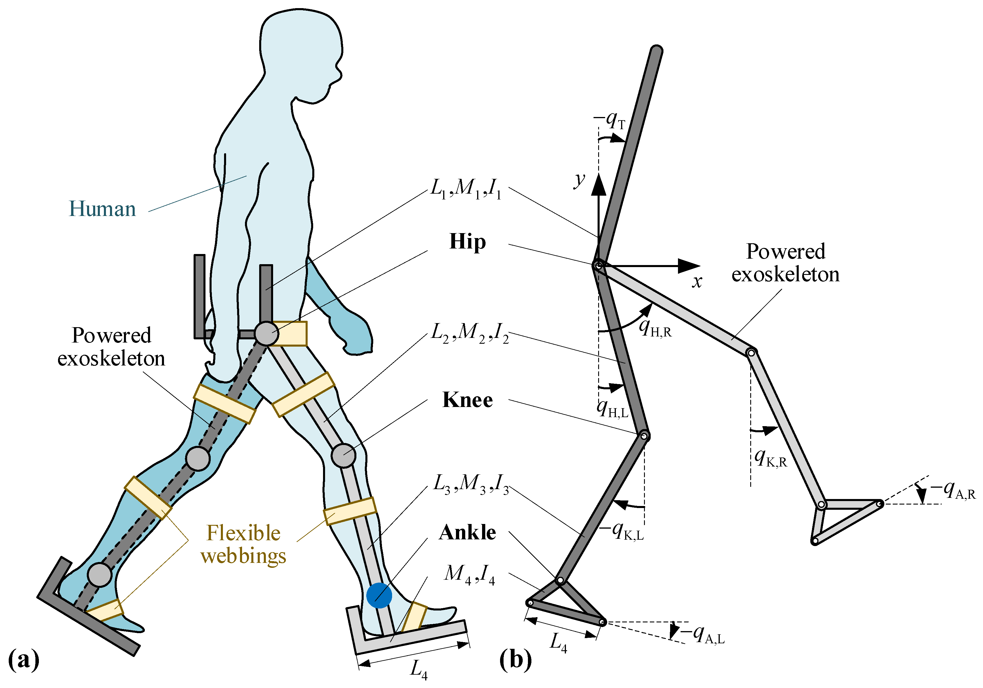
Figure 1a shows a human–exoskeleton system, in which the lower extremity exoskeleton consists of a trunk and two legs, and each leg is further divided into a thigh, a shank, and a foot. They connect through the hip, knee, and ankle joints. Generally, the exoskeleton integrates with the human body through flexible webbings. When a human walks along a straight line, only the motion in the sagittal plane is considered, and the motions in the coronal plane and the horizontal plane are neglected due to their small range [
44]. Hence, each hip/knee/ankle joint of the exoskeleton has only one DOF of flexion/extension, with the rotation axis being perpendicular to the sagittal plane. In addition, the trunk can pitch/tilt, and the exoskeleton as a whole has two DOF along the x and y directions in the sagittal plane; they apply to the rotation axis of the hip joints. In sum, the lower extremity exoskeleton can be described via a two-dimensional (2D) model with a total of nine DOFs (
Figure 1b); the trunk, the tights, and the shanks are simplified into rigid rods, and the foot is represented by a tetrahedron, which is a triangle in the sagittal plane.
For each part, the center of gravity is assumed to be located at the geometric center. For the trunk, the length, mass, and the moment of inertia about the center of gravity are denoted by , , and , respectively. For each thigh, shank, and foot of the exoskeleton, we denote their lengths by , , and , respectively, their masses by , , and , respectively, and the moments of inertia with respect to the corresponding centers of gravity by , , and , respectively. The angles of the trunk (), the thighs ( and ), and the shanks ( and ) are measured from the vertical axis, and the angles of the feet ( and ) are measured from the horizontal axis, with the counterclockwise direction defined as positive. In the above parameters, the subscripts ‘B’, ‘T’, ‘S’, and ‘F’ denote the trunk, the thighs, the shanks, and the feet, respectively, and the subscripts ‘L’ and ‘R’ denote the left and the right side, respectively. In this research, without the loss of generality, (, ), (, ), and (, ) are also used to denote the angles of the hip, the knee, and the ankle joints of the exoskeleton, respectively.
Note that the studied 9-DOF exoskeleton possesses seven joints to be controlled, which exceeds the technological level of the current powered lower extremity exoskeleton prototypes. The reason for studying such a hypothetical example is to demonstrate the capability of the proposed controller in tackling high-dimensional systems in a real-time manner, which will be discussed in
Section 3.
2.2. Dynamic Modeling
The controller to be constructed in this research does not depend on a prior dynamic model of the human–exoskeleton system. The purpose of modeling in this subsection is to provide a platform for the dynamic simulation experiments, based on which the effectiveness of the proposed controller can be examined, and the unique merits can be uncovered by comparing with the conventional PID control. Based on such purposes, the basic philosophy for modeling is to put as many uncertainty factors as possible into the model, providing that the developed model is numerically processible.
In previous research, the movement of the exoskeleton is always divided into the swinging phase and the stance phase, and they are modeled separately [
18,
45,
46,
47]; therefore, it is not necessary to directly describe the foot–ground interaction and the constraint force of the knee joint after the leg is straightened. In this research, the dynamics of the exoskeleton in a complete gait cycle are considered, and two strong nonlinear factors, i.e., the foot–ground interaction and the constraint force at the knee joints, are modeled and incorporated. In detail, the exoskeleton shown in
Figure 1b possesses nine DOFs, with the generalized coordinate vector
being assigned as
. The governing equation of the exoskeleton is derived via the Lagrange Equation of the second kind,
On the left-hand side of the governing equation,
is the mass matrix;
is the matrix for the Coriolis forces, the centrifugal forces, and the damping forces;
is a vector for the gravitational forces and the elastic restoring forces at the joints; on the right-hand side,
denotes the control torques;
indicates the human–exoskeleton interactions;
denotes the gravity compensation to modify the PID control; and
is the generalized force vector corresponding to the foot–ground interaction forces and the unilateral constraint forces of the knee joints, which can be expressed as follows:
where
and
(
) are the normal pressure and the friction force applied to the toe or heel of the exoskeleton foot, respectively; they together constitute the foot–ground interaction.
(
) denotes the unilateral constraint force of the left and right knee joints after the leg is straightened, which is essentially the contact force that originated from the angle-limit mechanism between the tight and shank rods of the exoskeleton.
is the Jacobian matrix that transforms the above forces into generalized forces.
In this research, the normal pressures
(
) are described using the smoothed Kelvin–Voigt model [
48]
and the friction forces
(
) are described by the smoothed Coulomb dry friction [
48].
In Equations (3) and (4),
and
are constants describing the degree of smoothing of the normal pressures and the friction forces;
and
are the stiffness and the damping of the contact, respectively;
is the dry friction coefficient;
is the tangential velocity of the toe or the heel with respect to the ground; and
denotes the virtual depth of the foot pressing into the ground, which equals zero when the foot is off the ground. The parameters of the foot-ground contact model are given according to [
49]. The unilateral constraint force
(
) of the knee joint is also described by the smoothed Kelvin–Voigt model as follows:
Similarly, is the constant describing the degree of smoothing; and are the stiffness and damping of the contact, respectively; and represents the virtual indentation depth between the thigh and shank rods.
Generally, the human-exoskeleton system involves uncertainties and would inevitably suffer disturbances; they can be reflected in the dynamic equation. On one hand, stiffness and damping are assumed at the exoskeleton joints for restoring, their coefficients may suffer fast or slowly varied changes (to be introduced in
Section 4). On the other hand, the human–exoskeleton interactions (i.e., the term
) are unknown in nature and the walking environment (reflected in
and
) subject to uncertainty. We will also consider scenarios in which the walking speed changes, which is reflected in the tracked trajectory.
2.3. Human Gait Kinematics Acquisition
The subject was fully explained of the aims and details of the protocol and voluntarily agreed in participation, with the signing of written informed consent. The purpose of the tests is to obtain the walking gait kinematics (
, the subscript ‘H’ denotes the human) of a healthy subject, which will be used in simulation experiments. The equipment used in the experiment includes the Cosmos Gaitway platform and Vicon optical motion capture system. The healthy subject is male, 180 cm in height and 90 kg in weight. Referring to the Helen Hayes model, the healthy subject was pasted with 18 targets. During the experiment, the subject walked on the Cosmos Gaitway with different slopes and different speeds. The sampling frequency of the optical motion capture system is 100 Hz. The final data obtained from the experiment are the spatial coordinates of each target. Then, the spatial coordinates of the hip joint and the spatial rotation angles of the hip, knee, and ankle joints can be obtained by using the angle solution method of the Helen Hayes model. Detailed gait kinematics acquisition and data decoding procedures can be found in [
50]. Different scenarios are set for the healthy subject, including variations of the treadmill speed and the treadmill inclination angle.
Based on the acquired gait kinematics
, the human joint torques can be calculated by inversely solving the dynamic model of the human. The governing equation can also be derived based on the Lagrange equation.
The terms on the left-hand side share the same meaning as those of Equation (1); on the right-hand side denotes the generalized forces corresponding to the foot–ground normal pressures, the foot–ground friction forces, and the joint torques. By substituting the gait kinematics and the measured normal pressures and friction forces, the joint torques expressed in terms of the generalized coordinates can be obtained.
3. PSO Based Online Adaptive PID Controller
The exoskeleton system shown in
Figure 1 is fundamentally a multiple DOF system, which possesses the following salient characteristics: parameter uncertainties, unknown human-exoskeleton interactions, external perturbations, and environment changes. Aiming at these features, a PSO-based online adaptive PID controller is proposed. Prior to this, the conventional PID tuning method and the standard PSO algorithm are introduced.
3.1. PID Tuning Based on Parameter Identification
The classical PID control law for trajectory tracking is
where
,
, and
are proportional, integral, and derivative gains of the PID controller, respectively. Here, the subscript
could take ‘B’, representing the trunk; ‘TR’ and ‘TL’, representing the right and left thigh, respectively; ‘SR’ and ‘SL’, representing the right and left shank, respectively; and ‘FR’ and ‘FL’, representing the right and left foot, respectively. In Equation (7),
is the tracking error in position, and
is the tracking error in velocity, they are given by the following:
where
and
denote the desired and the measured position, respectively,
and
denote the desired and the measured velocity, respectively.
Note that although the dynamic model of the exoskeleton is strongly nonlinear, the behaviors of the closed-loop system with the PID control are similar to the transient responses of a linear system [
51]. By applying the PID control, each joint (corresponding to a generalized coordinate) of the exoskeleton robot can be characterized by a single input single output (SISO) system. Under the range of motion (ROM) condition, by letting one joint move and freezing the other joints [
52], each joint can be approximated via a second-order linear system, which can be written as a transfer function in the frequency domain as follows:
Applying a step input, the plant gain
, the damping ratio
, and the time constant
can be identified. Hence, based on tuning formulas similar to the Ziegler–Nichols and Cohen–Coon methods [
51], the PID gains can be obtained.
3.2. Standard PSO Algorithm
Particle swarm optimization (PSO) is a population-based optimization technique inspired by swarm behavior such as bird flocking and schooling in nature. It is a metaheuristic that possesses the following merits: PSO requires few or no assumptions about the problem to be optimized, differentiability is not required by the optimization problem, and the solution space that can be searched can be very large. Due to these virtues, PSO is a powerful tool for multidimensional complex optimization problems.
In the standard PSO (SPSO) algorithm, the potential solutions, called particles, move in the search space following the current optimum particle. Basically, each particle (
) in the swarm (with
particles) at the
k-th iteration has two attributes, the position
and the velocity
. The movement of each particle is determined by a velocity term, which represents the attraction of its own best-known position (
) as well as the entire swarm’s best-known position (
) in the search space. Specifically, the velocity of each particle is updated based on Equation (10), in which
and
are the social learning factors (or, acceleration constants),
is the prescribed inertia weight, and
and
are random numbers between 0 and 1 in each iteration. The position of the particle can then be updated according to Equation (11). The iteration terminates when the prescribed number of iterations is reached, or the critical value of the objective function
is achieved.
3.3. PSO-Based Online PID Control
As introduced in
Section 2.1, the exoskeleton has seven joints to be controlled for trajectory tracking. This can be achieved via the PSO-based online PID control.
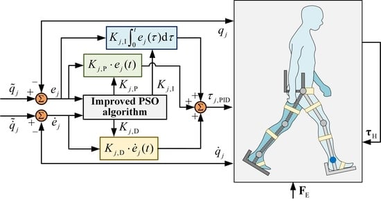
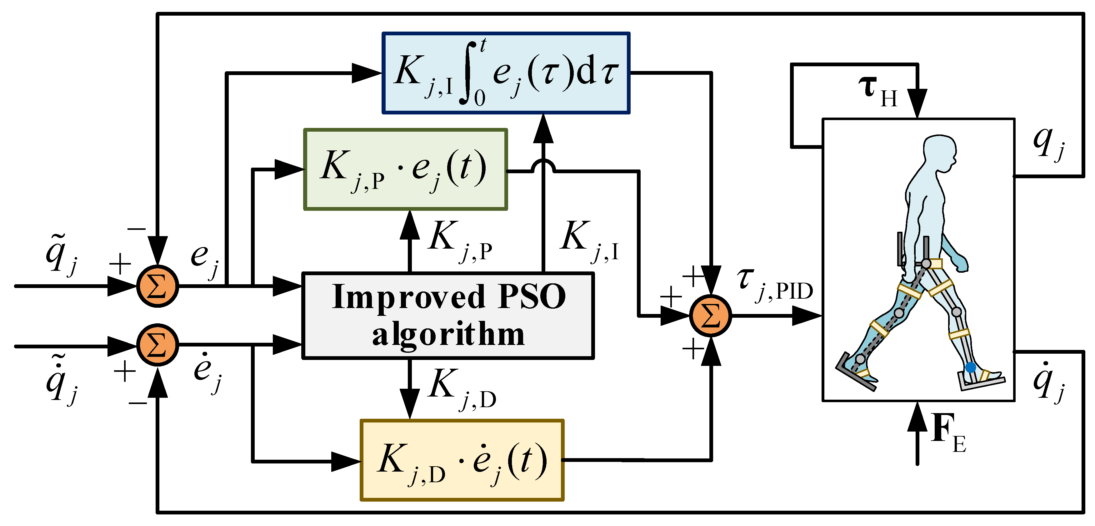
Figure 2 displays the block diagram of the controller. The core idea of the controller is to optimize the PID coefficients online via the PSO algorithm so that the tracking errors in both the position and the velocity can be converged in a short time. To this end, the objective function of the optimization problem is defined as follows:
which measures the mean accumulated error (MAE) in both the position and the velocity up to time
. Here, the subscript
could take ‘B’, ‘TR’, ‘TL’, ‘SR’, ‘SL’, ‘FR’, and ‘FL’.
Note that with the PID control (see the control law in Equation (7)), there are 21 parameters (i.e., proportional, integral, and derivative gains corresponding to the seven joints) to be optimized. PSO is an ideal tool for tackling such a high-dimensional problem. Hence, if with PSO, the search space is 21 dimensional, and each particle in the swarm (with particles) to be optimized is fundamentally a 21-dimensional vector of PID gains (i.e., ). Algorithm 1 provides the pseudo-code of using the standard PSO (SPSO) algorithm to optimize the PID coefficients online. To ensure that the controller could online update the PID coefficients, rather than evaluating all the particles of the swarm in an offline manner, each particle (i.e., a 21-dimensional vector of the PID gains) is directly injected into the human–exoskeleton system for control. Hence, within each time step, there is only one particle that serves as the PID gains to control the exoskeleton. In other words, it is not necessary to wait for the convergence to the best solution. This ensures the real-time implementation of the controller in a real exoskeleton system. When all the particles in the swarm (in this research, the population size is 100) are traversed, they will be updated based on their own best-known positions and the swarm’s best-known position. This is also a simple calculation that can be handled very soon by common control boards. Moreover, the controller can accurately track the desired trajectory by incorporating only the input () and output () of the system, without having to know the dynamic model and relevant prior knowledge of the system.
Although the SPSO algorithm is relatively simple and easy to implement, there are some limitations when applying it for nonlinear system control, especially when the system involves non-negligible uncertainties and unknown disturbances.
- (a)
Since the particles are generated randomly and the inertia weight remains unchanged for good global searching, the algorithm takes a long time to converge. During this convergence period, the control torques may be highly fluctuated due to the unstable PID gains, which would induce undesired vibrations of the exoskeleton and cause harm to the human body.
| Algorithm 1 Online PID control based on the standard PSO (SPSO) algorithm |
| 1: Start |
| 2: Initialize |
| 3: Initialize the swarm to random values |
| 4: while the experiment does not end do |
| 5: for do |
| 6: Inject a particle (with position and velocity ) |
| 7: Calculate control torques using Equation (7) |
| 8: Apply to the human-exoskeleton system |
| 9: Evaluate the objective function
|
| 10: Save and the corresponding value of |
| 11: Update and |
| 12: end for |
| 13: Update the swarm (with particles) by Equations (10) and (11) |
| 14: end while |
| 15: End |
- (b)
The SPSO algorithm may encounter premature convergence. That is, when the algorithm converges, the SPSO algorithm lacks the adequate capability to let the particles leave the local optimum and to re-search for better solutions. This is particularly vital when the system suffers abrupt changes (e.g., parameter perturbations, unknown human dynamics, and environmental disturbances, etc.) and the current solution is no longer the optimum.
In the following subsection, improvements are incorporated into the PSO algorithm, for tackling the above two issues.
3.4. Online Adaptive PID Control Based on Improved PSO Algorithm
Generally, the human–exoskeleton system is subject to uncertainties and disturbances, including unknown human–exoskeleton interactions, uncertain joint stiffness and damping, environment changes, and variations of the tracked trajectory, etc. These factors would significantly diminish the effectiveness of the standard PSO (SPSO) algorithm due to the abovementioned limitations. To overcome these issues, an improved PSO (IPSO) algorithm is proposed and incorporated into the controller. Algorithm 2 displays the pseudo-code of the online adaptive PID controller based on the IPSO algorithm. Improvements of the PSO algorithm mainly fall into the following two aspects:
First, to achieve a balance between the global and local search capability, the inertia weight
is asked to decrease stochastically in the initial stage (say, 2 s). Specifically, the inertia weight
follows a normal distribution with the mean decreasing linearly from 2 to 0.6, and the standard deviation equaling 2. After the initial stage, the inertia weight
stays at a relatively low value of 0.6 to ensure good local search capability. In addition, to improve the searching efficiency, the particle (i.e., the PID gains) obtained through the classical tuning method (introduced in
Section 3.1) is forced to be involved in the swarm.
Second, and the most significant, to prevent premature convergence in the context of perturbations and disturbances, a ‘leaving and re-searching’ mechanism is introduced into the controller. In detail, two critical conditions are included. The first is as follows:
where
is the standard deviation of the particle velocities, quantifying the velocity discrepancy among the particles. When
drops below a prescribed small value
, we can presume that the swarm is converged. The second condition is as follows:
which quantifies the variation tendency of the mean accumulated error. If the ratio is higher than a prescribed value
, which is a constant greater than one, we can presume that the control applied at time
is not optimum. This can be induced by certain interferences originating from the system itself or the environment.
If either condition (13) or (14) does not hold (i.e., the swarm has not converged (condition (13) is violated) and/or the control applied at time is the optimum (condition (14) is violated)), steps in Algorithm 2 (which is similar to the online PID control based on the SPSO algorithm, i.e., steps in Algorithm 1, except that the inertia weight is updated each time after the iteration) will be executed. On the other hand, if both conditions are satisfied, i.e., the solution after convergence is not the optimum one, the ‘leaving and re-searching’ mechanism (steps in Algorithm 2) is executed. Specifically, we randomly select particles (e.g., ) and let them re-search in the neighborhood of the current converged values to decrease the objective function (i.e., to locate a new optimum solution).
The domain for local search is a 21-dimensional supra-sphere with radius
, and the positions of the selected particles are initialized via the following:
where
is a vector of random numbers between
and
. Here, the random numbers corresponding to
,
, and
are assumed to be identical, respectively. Each time when the
particles are evaluated, the corresponding best-known position of the particle
(
) and the best-known position of the entire swarm (
) will be updated. Due to the relatively small number of particles and the limited search space, as well as with a stochastically decreasing inertia weight
, the convergence condition (13) can always be satisfied. However, the local search will continue until the condition (14) is no longer met. Thereupon, the positions of all the particles in the whole swarm (with
particles) will be forcefully replaced by
, and the evolution returns to steps
.
Algorithm 2 also indicates that the improved PSO algorithm is a linear time algorithm with time complexity
. This means that the running time increases, at most, linearly with the number of particles
in the swarm. Moreover, an increase in the DOF of the controlled system does not affect the time complexity of the algorithm. In sum, it can be hypothesized that the resources required by the proposed algorithm are low, which makes it feasible to deploy on an online controller.
| Algorithm 2 Online adaptive PID control based on improved PSO (IPSO) algorithm |
| 1: Start |
| 2: Initialize
and |
| 3: Initialize the swarm to random values; the particle corresponding to pre-tuned PID gains is forced to involve |
| 4: for do |
| 5: Inject a particle (with position and velocity ) |
| 6: Calculate control torques using Equation (7) |
| 7: Apply to the human–exoskeleton system |
| 8: Evaluate the objective function by Equation (12) |
| 9: Save and the corresponding value of |
| 10: Update and |
| 11: end for |
| 12: Update the swarm (with particles) by Equations (10) and (11) |
| 13: Update the inertia weight |
| 14: while the experiment does not end do |
| 15: if (conditions given by Equations (13) and (14) hold) then |
| 16: Randomly select particles; initialize them randomly based on Equation (15) |
| 17: for do |
| 18: |
| 19: end for |
| 20: Update the sub-swarm (with particles) by Equations (10) and (11) |
|
21: Update the local inertia weight |
| 22: if (condition given by Equation (14) hold) then |
| 23: GOTO 17: |
| 24: else |
| 25: All particles in the swarm (with particles) are replaced by |
| 26: |
| 27: end if |
| 28: else |
| 29: |
| 30: end if |
| 31: end while |
| 32: End |
4. Results
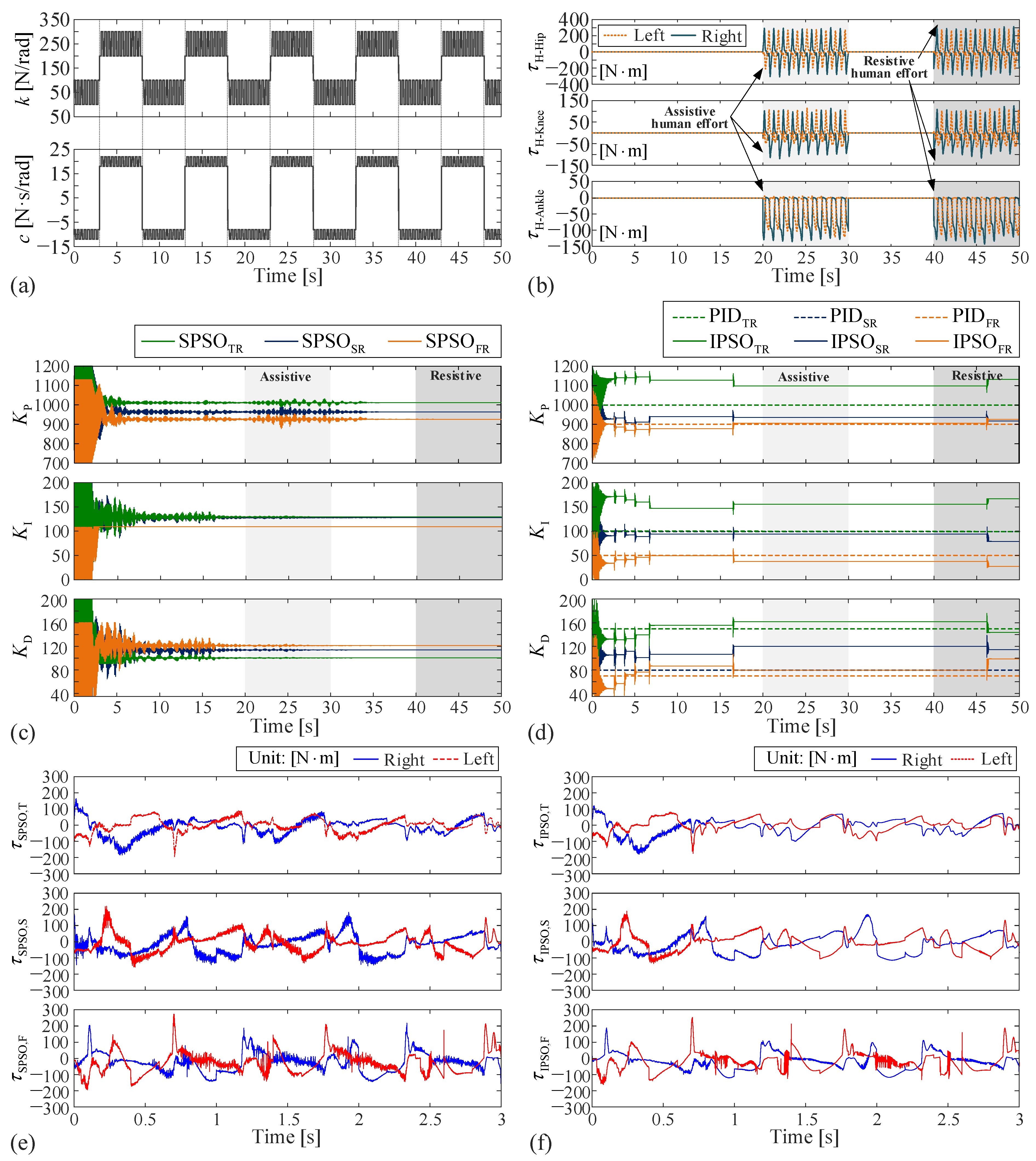
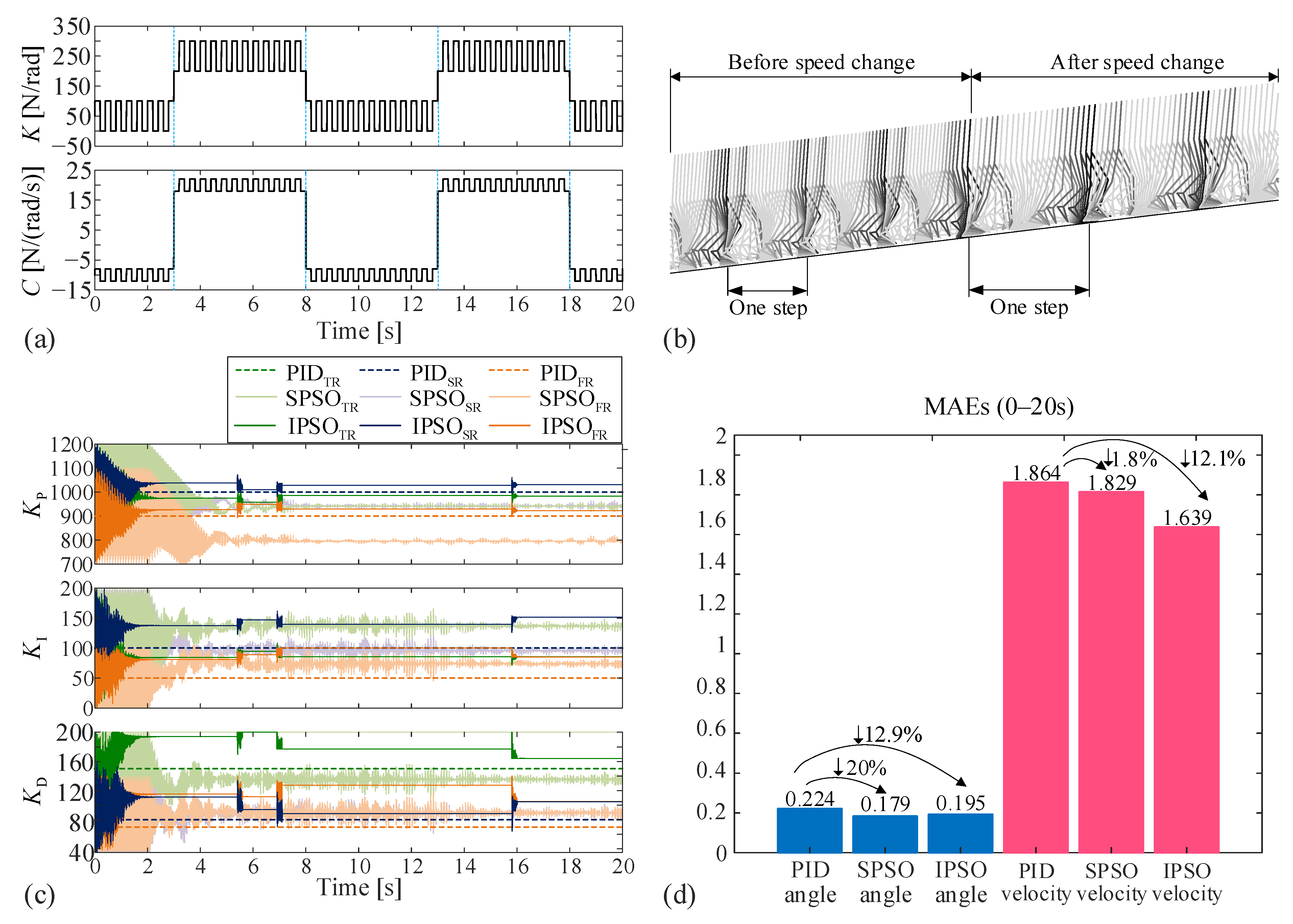
This section examines the performance of the proposed controller for trajectory tracking in various scenarios. The following four cases are studied in detail: (1) walking on a horizontal plane with unknown human-exoskeleton interactions, (2) walking on a horizontal plane with variable speed, (3) walking uphill and downhill, and (4) walking uphill with variable speed. The model parameter uncertainties are also taken into considerations. We assume that the stiffness and damping of the seven exoskeleton joints are subject to fast varying (with a frequency of 10 Hz, stiffness amplitude of 50 N/rad, and damping amplitude of 2
) and slow varying (with a frequency of 0.4 Hz, stiffness amplitude of 100 N/rad, and damping amplitude of 15
) perturbations (
Figure 3a), given by the following:
Unless otherwise stated, this assumption applies to all four cases to demonstrate the capability of the proposed controller in coping with non-negligible parameter uncertainties.
For comparison purposes, the conventional PID control with pre-tuned gains will also be tested in the abovementioned cases. We will demonstrate that the proposed controller based on the IPSO algorithm could significantly improve the tracking accuracy in both the position and the velocity. Moreover, with the introduced improvements, the limitations of the SPSO algorithm can be overcome.
The four cases will be examined through numerical simulations. Specifically, the tracking signals are obtained through experiments introduced in
Section 2.3; when the control torques are generated via the controller, they will be injected into the dynamic model governed by Equation (1). The dynamic model will be solved in MATLAB 2018b via the forward Euler method with step size 0.0001 s, which mimics the behavior of a real human-exoskeleton system. The sampling rate of the controller is 100 Hz, which can be easily achieved by common control boards. In the IPSO algorithm, the number of particles
. Compared with the traditional offline PSO, the population size is small. This is because, in this research, the PSO is implemented in a real-time manner. Each particle is used as the PID gains to control the exoskeleton in each time step, and the iteration is carried out after all the particles in the population are traversed. To ensure the sensitivity of the controller to interference, the population should not be too large. In the ‘leaving and re-searching’ mechanism, the critical values are set as
,
, and the number of particles for local search is
. The saturation torque of the exoskeleton is set as
.
4.1. Case I: Walking on a Horizontal Plane with Unknown Human–Exoskeleton Interactions
In the first case, the controller is expected to track the position and velocity of the human when walking on a horizontal treadmill with a speed of 1.0 m/s. The human efforts, which could be either resistive or assistive to the exoskeleton, are put into consideration. They are expressed as the joint torques in terms of the generalized coordinates (obtained via the method introduced in
Section 2.3). Fundamentally, they are unknown and unpredictable a priori. In this case, for simulation purposes, we assume that the human body provides assistive efforts to the exoskeleton during 20–30 s, with 75% of the human joint torques (including the torques at the hip, the knee, and the ankle joints) being applied to the exoskeleton joints; during 40–50 s, we assume that the human body resists the exoskeleton’s motion, with 75% of the reverse human joint torques being applied to the exoskeleton joints. The applied joint torques are plotted in
Figure 3b; they need to be transformed to the generalized forces before being substituted into the governing equation.
This case is tackled via the proposed online adaptive PID control based on the IPSO algorithm. To demonstrate its merits, another two control methods, i.e., the conventional PID control with pre-tuned gains and the online PID control based on the SPSO algorithm, are also tested and compared. For both the SPSO and the IPSO algorithms, the search space is determined based on the pre-tuned PID gains (
,
, and
). Specifically, for the knee and the ankle joints, we have the following:
Here,
is not allowed to take values lower than 35 to prevent possible instability. For the hip joints, the derivative gain is adjusted into the following:
where the proportional and integral gains remain the same as Equation (18). In what follows, unless otherwise stated, the search space defined in Equations (17) and (18) also apply to the other cases.
Figure 3c,d demonstrate how the PID coefficients evolve with respect to the time when the three controllers are applied, respectively. Overall, at the initial stage of simulation, both the SPSO and the IPSO algorithms have shown their abilities to dynamically adjust the PID gains. Although the PID coefficients vary sharply in the convergence stage, the control performance is largely good (
Figure 4). This is because the search space of the particles (i.e., the search space of the PID coefficients) is determined according to the pre-tuned results, and stability can be ensured when the particles locate within the search space. After convergence, the converged PID gains are different from the pre-tuned values, indicating a performance improvement of the trajectory tracking brought by the PSO algorithm. However, in terms of the convergence speed and the chattering phenomena, the IPSO algorithm is significantly superior to the SPSO algorithm. With a stochastically decreasing inertia weight
w, the IPSO algorithm converges quickly in about 2 s, while the SPSO algorithm needs more than 5 s to reach a full convergence. Moreover,
Figure 3c,d show clearly that the SPSO algorithm induces noteworthy chattering of the PID gains during the converging stage and even during the middle stage (e.g., from 20 to 35 s for
), while the IPSO algorithm could effectively suppress such chattering.
Furthermore, with the ‘leaving and re-searching’ mechanism, after the convergence (say, 0 to 2 s), the IPSO algorithm will constantly initiate local searches to restrain the increase rate of the objective function value induced by fast and slow variations of the model parameters and human–exoskeleton interactions. For example, the adjustment of the PID gains that happened at 16.5 s is induced by the increase in the error change rate caused by tracking error accumulation due to the fast and slow varying of the parameters. This PID gain adjustment does not relate to the assistive human efforts during 20–30 s. The adjustment of the PID gains at 46.2 s is also induced by the increase in the error change rate caused by tracking error accumulation. However, here, the errors come from both the resistive human efforts and the parameter changes. On the contrary, the SPSO algorithm fails to adaptively adjust the PID gains even when substantial parameter variations or human–exoskeleton interactions are encountered; it would easily stagnate in a local optimum after convergence.
Correspondingly,
Figure 3e,f display the time histories (0–3 s) of the control torques of the exoskeleton corresponding to the SPSO and the IPSO algorithms, respectively. When the SPSO algorithm is employed, significant chattering phenomena are observed during the converging stage (0–3 s). However, when the IPSO algorithm is employed, such chattering is notably suppressed; for the hip and the knee joints, chattering is restrained in less than 1 s.
To demonstrate the effects of the proposed online adaptive PID control based on the IPSO algorithm,
Figure 4a–f display the tracking errors in both the position and the velocity corresponding to the right hip, the right knee, and the right ankle. It reveals that the proposed controller could ensure good tracking performance in the stages when the model parameters change sharply, or assistive/resistive human effects are applied.
Figure 4a–f indicate that the tracking errors are greatly affected by the model parameter variations, which cannot be completely suppressed by adjusting the PID coefficients via the IPSO algorithm. Moreover, during the stage with resistive human effects, the exoskeleton joints output higher torques to oppose the resistive effects and to ensure the tracking performance.
To further quantify the accuracy, the objective function, i.e., the MAE, is examined. The first stable stage (10–20 s), the stage with an assistive human effect (30–40 s), the stage with a resistive human effect (40–50 s), and the whole process (0–50 s) are studied separately. A comparison of the results indicates that the PID coefficients obtained via the model-based tuning method perform well in angle tracking, and the SPSO algorithm could provide a low level (<5%) reduction in the MAE in position. Due to the torque chattering caused by SPSO (which will cause great damage to the motor), Therefore, considered comprehensively, it cannot be used as a real-time control algorithm. With the IPSO algorithm, the decrease in the MAE in position becomes more significant. On the other hand, in terms of velocity tracking, the merits of incorporating the PSO are obvious. Particularly, in all the examined stages, the IPSO algorithm could achieve more than a 16% decline of the MAE in velocity. The reduction in the MAE is the highest when both model parameter variation and human interference exist, manifesting the capability of the proposed controller in coping with strong perturbations.
4.2. Case II: Walking on a Horizontal Plane with Variable Speed
In case II, the controller is expected to track the position and velocity of the human walking on a horizontal treadmill with varying speeds. Specifically, the human first walks on a horizontal treadmill at 1.2 m/s for 5 s, and then jogs at 1.8 m/s. The stiffness and damping coefficients of the exoskeleton joint are still subject to fast and slow variations determined by Equation (16), shown in
Figure 5a. This case is studied via the following two methods: the conventional PID control with pre-tuned coefficients and the proposed online adaptive PID control based on the IPSO algorithm.
With the proposed controller, the human–exoskeleton system could effectively track the given signals.
Figure 5b displays a stroboscopic image of the exoskeleton motion before and after the speed change in seven gait cycles. The stride length after the speed change is obviously longer than that before the speed change.
Figure 5c shows the real-time evolution of the PID coefficients during the simulation process. It reveals that the IPSO algorithm could locate an optimal solution that is different from the pre-tuned one in about 2 s. After that, during 3–8 s, the model parameters are substantially increased, and the walking speed changes from 1.2 to 1.8 m/s, these two factors would significantly increase the MAE values. Consequently, the ‘leaving and re-searching’ mechanism is activated several times during this stage to locally search the PID coefficients so that the increase in the objective function can be held back, and the tracking accuracy can be ensured. Activation of the ‘leaving and re-searching’ mechanism is also observed during 13–18 s due to the substantial rise of the model parameters.
Figure 5d quantifies the MAEs in both the position and the velocity corresponding to the three control methods. It shows that the SPSO algorithm could also improve (or equate with) the tracking performance based on the conventional PID, although the improvement is limited when compared with the
IPSO algorithm. For example, the SPSO algorithm acquires a 3.6% reduction in MAE in position, which is lower than that for the IPSO algorithm (5.8%). In terms of the MAE in velocity, the SPSO induces a 7% reduction, while the IPSO algorithm could achieve a 20.4% reduction. These results indicate that the IPSO algorithm outstrips the SPSO algorithm. Moreover, the IPSO algorithm could effectively restrain the chattering of the control torques, which makes it become a better choice than the SPSO algorithm.
4.3. Case III: Walking Uphill and Downhill
In Case III, during 0–10 s, the human walks uphill at 0.6 m/s on a 10% gradient treadmill; during 20–30 s, the human walks at 1 m/s on a horizontal treadmill, and during 20–30 s, the human walks downhill at 0.6 m/s on a –10% gradient treadmill. Hence, in this case, the environment change is reflected in both the tracked trajectory and the contact force between the foot and the ground (the models of the normal pressure and the friction remain unchanged, but the force directions change). Again, the stiffness and damping coefficients are assumed to suffer fast and slow variations determined by Equation (16), shown in
Figure 6a. Case III is examined by both the conventional PID control with pre-tuned gains and the online adaptive PID control based on the IPSO algorithm.
Numerical simulations reveal that the proposed controller could effectively track the signals for uphill, horizontal, and downhill walking.
Figure 6b displays a stroboscopic image of the exoskeleton motion during the whole process, in which the posture changes and the stride length differences among the three stages can be observed. During the 0–10-second uphill stage, the exoskeleton body leans forward, and the stride length is short; during 20–30 s, the stride length is longest; and during the 20–30-second downhill stage, the exoskeleton body leans backward, and the stride length is short again.
Figure 6c demonstrates how the PID coefficients are adjusted using the IPSO algorithm. With the ‘leaving and re-searching’ mechanism, after convergence at about 2 s, a local search of the PID gains is activated twice during 3–8 s due to the drastic variations of the model parameters. At about 10 and 20 s, local searches are activated again, which are caused by the increases in the MAE induced by environment changes (i.e., the terrain changes from uphill to level at 10 s, and changes from level to downhill at about 20 s) and speed changes.
We also evaluate the MAEs during the three stages and the whole process corresponding to the two control methods.
Figure 6d reveals again that the IPSO algorithm has a significant effect in improving the tracking accuracy of the angular velocity. During the whole process, a 15.0% reduction in the MAE in velocity is achieved when compared with the conventional PID control.
4.4. Case IV: Walking Uphill with Variable Speed
In Case IV, a scenario that the human walks uphill (10% gradient treadmill) with variable speed from 1.2 to 1.8 m/s is evaluated. Variations of the stiffness and damping coefficients are still assumed in this case, as shown in
Figure 7a. Case IV is examined by both the conventional PID control with pre-tuned gains and the online adaptive PID control based on the IPSO algorithm. Similarly, through the stroboscopic image (
Figure 7b), the evolution of the PID coefficients (
Figure 7c), and the bar charts of the MAEs (
Figure 7d), the effect of the proposed controller can be verified. During the whole process, the ‘leaving and re-searching mechanism’ is activated several times due to the sharp parameter changes and the speed change, which therefore lowers the MAE in position (by 12.9%) and MAE in velocity (by 12.1%) and guarantees the tracking accuracy.
4.5. Summary
Based on the dynamic model of the human–exoskeleton system (established in
Section 2), the performance of the proposed control method (i.e., the online adaptive PID control based on the IPSO algorithm) has been examined in four typical cases. Characteristic scenarios, including fast and slow variations of the model parameters (i.e., model uncertainties, in all cases), unknown human–exoskeleton interactions (Case I), environment changes (i.e., external disturbances, Case III), and switch of motion states (i.e., changes of tracked signals, Case II and IV) have been considered. The simulation results indicate that the proposed control method possesses two unique merits over the conventional PID control with pre-tuned gains and the PID control based on the SPSO algorithm. On one hand, by asking the inertia weight to decrease stochastically in the initial stage, the incorporated IPSO algorithm significantly outstrips the SPSO algorithm in achieving fast convergence and suppressing undesirable chattering phenomena (demonstrated in Case I). On the other hand, by activating local searches of the PID gains based on the ‘leaving and re-searching’ mechanism, the IPSO algorithm could effectively resist the increase in the objective function (i.e., the MAE) that originated from the unknown uncertainties and perturbations. The proposed controller also surpasses the conventional PID control with pre-tuned gains and the PID control based on the SPSO algorithm in terms of the tracking accuracy, which are evaluated by the MAEs in angle and angular velocity. Overall, through the four case studies in this section, the distinct advantages are uncovered. The proposed controller does not call for prior knowledge of the system; it could adjust the control gains effectively and timely to adapt to new environments and new tracked signals when the human–exoskeleton system is subjected to various model uncertainties, internal/external disturbances, and motion state changes.
5. Using the Controller to Achieve Lower Power Mode
After years of technology accumulation and development, many advanced exoskeleton robots have been proposed for rehabilitation or augmentation; however, they generally consume a lot of energy to achieve the functional objectives [
53]. Frequently, the battery life required by long-term high-intensity work is insufficient. Even on a level road, it is still a challenge to let the exoskeleton robot consistently assist humans walking for a long time. Hence, we consider if the proposed controller could reduce the output power and let the exoskeleton robot work in a lower power mode, providing that the tracking performance is not degraded. Here, to evaluate the control performance, the average output power (AOP) of the exoskeleton is defined and examined.
in which
could take ‘B’, ‘TR’, ‘TL’, ‘SR’, ‘SL’, ‘FR’, and ‘FL’.
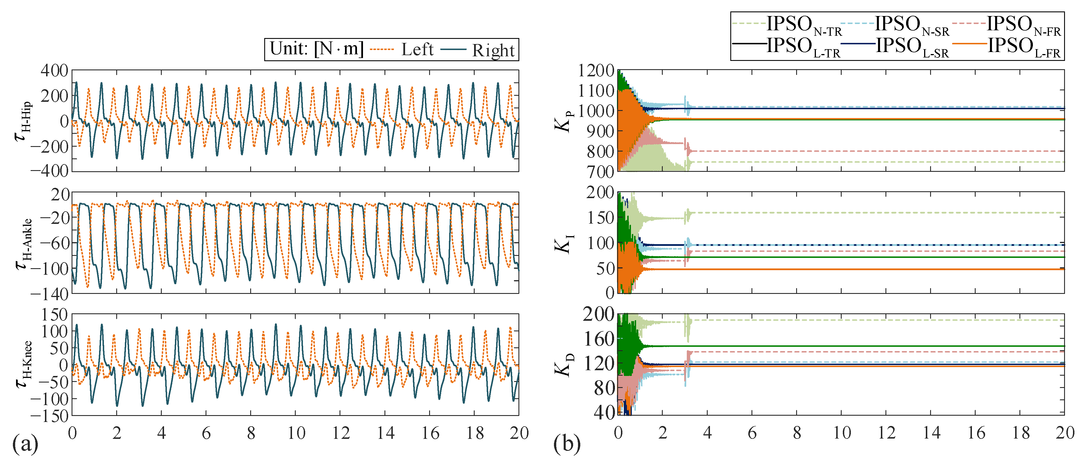
In the normal mode, the motion of the human–exoskeleton system is completely generated by the exoskeleton joints; in this mode, significant energy of the exoskeleton will be consumed, while the user will be fully relaxed under ideal conditions. In the low power mode, both the human joints and the exoskeleton joints contribute positively to the motion; in this mode, the human is assumed to move as in the unequipped state (i.e., human joints output 100% torque as the exoskeleton was not equipped), and the exoskeleton consumes less energy to just follow the human’s motion.
To demonstrate the performance difference, the normal mode and the lower power mode are evaluated and compared numerically. Here, zero joint stiffness and damping are assumed. In the normal mode, the simulation is performed without applying human joint torques, while in the lower power mode, 100% human joint torques (including the torques at the hip, the knee, and the ankle joints, obtained from the human gait test corresponding to walking on a horizontal treadmill with speed 1.0 m/s) are applied to the exoskeleton joints (
Figure 8a). The torques are transformed into the generalized forces for being substituted into the governing equation.
Figure 8b displays the evolutions of the PID coefficients (within the 20 s) corresponding to the normal mode and the low power mode under the IPSO algorithm. It shows that in the low power mode, the PID coefficients are converged to completely different values from those in the normal mode. After convergence, the PID gains remain stable since the system does not suffer any external perturbations. As a consequence, the AOP of the exoskeleton in the low power mode is about 25.0% lower (194.35 W) than that in the normal mode (259.26 W), which indicates effective energy saving. With this, the user would be able to switch the working mode of the exoskeleton according to his/her physical condition, the mission requirement, and the battery life.
6. Discussion
The discussion part mainly covers the following three aspects: tracking accuracy comparison, control system stability, a comparison of two algorithms in adjusting PID gains and the triggering of the ‘leaving and re-searching’ mechanism.
- (1)
To demonstrate the effectiveness of the proposed controller, the tracking performance is compared with several other control methods in the discussion part, in terms of the position tracking error level. In Khamar et al. [
24], the sliding mode control and an observer were integrated for a knee exoskeleton, which receives a satisfactory tracking effect. Jabbari et al. [
29] used a neural network to compensate for the unknown nonlinear dynamics of a knee exoskeleton. Oktaviani et al. [
35] designed a fuzzy active disturbance rejection controller for a hip and knee exoskeleton, and Liu et al. [
54] proposed an impedance controller with variable gains for a knee exoskeleton. The tracking performance is provided in
Table 1. For comparison purposes, the additional situational experiment is performed, in which the human–exoskeleton system is asked to follow the signals of human walking on a horizontal plane with a constant speed of 1.0 m/s, and the stiffness and damping parameters subject to small perturbations, given by the following:
Table 1 reveals that with small parameter perturbations, our IPSO-based PID controller is comparable with other methods, with the position tracking error ranging between the hip and the knee. The error for the ankle is a little higher than the hip and knee because of the foot–ground reaction forces. However, reports on ankle exoskeletons are rare, and a comparison cannot be made. With fast and slow varying perturbations of the stiffness and damping parameters (Equation (16)), as well as assistive or resistive human efforts (i.e., Case I), the tracking errors are increased, while the tracking performance is still acceptable.
Table 1, thus, verifies the effectiveness and the accuracy of the proposed IPSO-based PID controller.
In addition to the comparable tracking error level, the proposed controller possesses some unique merits. The controller does not require an accurate dynamic model or precise system parameters a priori; the controller could deal with high-dimensional systems; the controller could also suppress undesired chattering and adapt to various tasks/environments. Moreover, due to the simplicity and the real-time feature, the controller is promising to be deployed in a practical exoskeleton system.
- (2)
As for the stability of the controller, first, the particle range is obtained according to the pre-tuned PID gains obtained via the tuning formulas similar to the Ziegler–Nichols and Cohen–Coon methods [
51] (introduced in
Section 3.1). Based on Lyapunov stability analysis [
51], PID gains within this range can make the system stable. Second, as a classical metaheuristic algorithm, the convergence of the PSO algorithm has been systematically investigated in [
55,
56,
57]. These studies show that the particles will converge to a certain point in the search space without divergence. However, this converged point may or may not be optimum. Note that the convergence to the local optimum has been tackled via different methods, including the Lyapunov stability method [
58] and the von Neumann stability criterion [
59]. Due to the above two reasons, the stability of the controller can be well ensured. This is manifested in the five examples in this research. Note that the stability issue of the PSO itself falls out of the scope of this research, and thus is not provided in the manuscript.
- (3)
By comparing the PID gain evolution based on the SPSO algorithm and the IPSO algorithm (
Figure 3,
Figure 5,
Figure 6 and
Figure 7), the superiority of the IPSO algorithm in convergence speed and chattering suppression is revealed. The IPSO algorithm usually converges quickly in about 2 s in the initial stage, while the SPSO algorithm needs more than 5 s to reach a full convergence. Moreover, with the SPSO algorithm, significant chattering of the PID gains in both the convergence stage and the steady-state stage is observed, while with the IPSO, such chattering is effectively suppressed, which is favorable to stable control torque. Moreover, considering that the IPSO algorithm allows the PID gains to jump out of the local optimal solution based on the incorporated ‘leaving and re-searching’ mechanism, its adaptivity, with respect to parameter perturbations and working condition changes, is further improved.
- (4)
With the IPSO-based PID controller, adjustments of the PID gains after convergence is caused by the ‘leaving and re-searching’ mechanism. The triggering of this mechanism is determined by the variation tendency of the mean accumulated error but is not directly related to a specific walking condition change. Specifically, if the critical condition (i.e., Equation (14)) is satisfied, we can presume that the control applied at the time is not optimum. Satisfaction of the critical condition can be induced by the following two kinds of reasons: (1) a sudden surge of the error caused by sharp parameter changes, large external disturbances, or significant working condition variations; (2) an increase in the error change rate induced by error accumulation.
In order to apply the IPSO-based PID controller in a real-time scenario, the critical value needs to be carefully prescribed. An overlarge would let the mechanism insensitive so that the algorithm would lose adequate adaptability and trap into a local optimum; otherwise, if is very close to 1, the algorithm would become overly sensitive, which would induce undesired chattering of the PID gains. Therefore, rather than a constant value, should be selected case-by-case.
7. Conclusions
An IPSO-based model-independent adaptive PID controller is proposed in this paper, based on which, the human–exoskeleton system could operate effectively for trajectory tracking, which is demonstrated via numerical simulations in a few characteristic scenarios.
The most significant algorithm improvement lies in the introduction of the ‘leaving and re-searching’ mechanism. The essence of the mechanism is to test whether the currently converged solution is still optimum; if not, the converged particles will be asked to leave their current positions and to re-search locally for a better solution, such that the objective function value decreases.
To manifest the unique merits of the proposed controller, simulation experiments in four characteristic working scenarios are performed, which are based on a 9-DOF first-principle dynamic model of the exoskeleton robot. Specifically, the control performance is compared with those obtained from the conventional PID control with pre-tuned gains and the online PID control based on the SPSO algorithm. Specifically, the IPSO was based on adaptive PID controller features with the following virtues: a relatively faster convergence, suppression of the chattering phenomena, real-time adjustment of the PID gains when subjected to interferences, and significantly reduced tracking errors. We also provide an example to demonstrate that the proposed controller can be exploited for letting the exoskeleton work in an energy-saving low power mode.
Finally, we list a few directions of future work by introspecting the limitations of this research. (1) Experimental verification is not performed in this research, partly due to the lack of a mature 7-DOF exoskeleton prototype. It is necessary to experimentally verify the effectiveness of the proposed controller in a reduced DOF exoskeleton prototype in future research. Moreover, we believe that there is no impediment to implement the proposed controller in complex 7-DOF exoskeleton prototypes because of its low requirement of computing resources. (2) Due to the metaheuristic nature of the PSO algorithm, the obtained PID gains for each test would be necessarily different. In the simulations, we notice that such differences do not substantially deteriorate the control performance. However, when applying the proposed IPSO-based online PID controller to a practical exoskeleton, the possible destabilization should be considered, and it would be necessary to provide theoretical evidence to prove the stability. (3) The control performance also relies on the physical parameters of the exoskeleton; if the exoskeleton itself is poor in dynamic stability and energy efficiency, the IPSO algorithm would hardly improve the control performance. This, therefore, calls for efforts in exoskeleton design optimization.


