Article

Discrete and Fuzzy Models of Time Series in the Tasks of Forecasting and Diagnostics

Department of Information Systems, Ulyanovsk State Technical University, 432027 Ulyanovsk, Russia
*
Author to whom correspondence should be addressed.
Axioms 2020, 9(2), 49; https://doi.org/10.3390/axioms9020049
Submission received: 30 March 2020 / Revised: 22 April 2020 / Accepted: 27 April 2020 / Published: 30 April 2020
(This article belongs to the Special Issue Fuzzy Systems for Data Managing in Business, Society, and Economics)

Abstract

:
The development of the economy and the transition to industry 4.0 creates new challenges for artificial intelligence methods. Such challenges include the processing of large volumes of data, the analysis of various dynamic indicators, the discovery of complex dependencies in the accumulated data, and the forecasting of the state of processes. The main point of this study is the development of a set of analytical and prognostic methods. The methods described in this article based on fuzzy logic, statistic, and time series data mining, because data extracted from dynamic systems are initially incomplete and have a high degree of uncertainty. The ultimate goal of the study is to improve the quality of data analysis in industrial and economic systems. The advantages of the proposed methods are flexibility and orientation to the high interpretability of dynamic data. The high level of the interpretability and interoperability of dynamic data is achieved due to a combination of time series data mining and knowledge base engineering methods. The merging of a set of rules extracted from the time series and knowledge base rules allow for making a forecast in case of insufficiency of the length and nature of the time series. The proposed methods are also based on the summarization of the results of processes modeling for diagnosing technical systems, forecasting of the economic condition of enterprises, and approaches to the technological preparation of production in a multi-productive production program with the application of type 2 fuzzy sets for time series modeling. Intelligent systems based on the proposed methods demonstrate an increase in the quality and stability of their functioning. This article contains a set of experiments to approve this statement.

1. Introduction

The tasks of behavior research on complex organizational and technical systems are currently reduced to analysis of the history of their construction. Large volumes of data accumulated in the databases of information systems are the basis for such analysis. Statistical information has always been important for various industries. Identification of patterns in the process of analyzing large amounts of data allows to receive information to the systems management [1].
There are two approaches to working with data that can be recognized from that kind of analysis:
  • Collection and conversion of existing accumulated data (a priori data) into a form appropriate for analyzing the history of objects from the current subject area.
  • Purposeful preservation of the dynamics of changes in the state of the studied objects.
The investigated objects can be represented for analysis as time series of their indicators.
A time series is defined as a sequence of values ordered in time and characterizing the level of state and changes in the observed indicator [2,3].
A feature of the time series, in contrast to a simple set of statistical data, is the dependence of the indicator value on its past states [3]. The order of the values is significant in the time series.
Time series differ in the following attributes:
  • Length of the series. The length of the series is usually described as the number of observations of the parameter. Sometimes the length of the series may also mean the time elapsed from the initial to the final observation [4]. Kendel writes in [4] that in contrast with statistics in time series analysis the amount of information is not proportional to the number of sample members, because “… sequential quantities are not independent.”
  • Discreteness and continuity. Discreteness and continuity is determined by the nature of the changes in time during which the observation is made. Discrete time series can be obtained from continuous time series in two ways [3]:
    • With sampling of values from continuous time series at a specific interval;
    • With the accumulation of values over a period of time.
  • Determinacy. The time series is called deterministic when the future values of the time series are determined by any mathematical function. The time series is called non-deterministic, random or stochastic, if future values are described only by the probability distribution. The stochastic time series can be stationary or non-stationary. A time series is called stationary if its properties are independent of the start point of the time. In particular, it has [3]:
    • Constant expected value (the average value with relation to which it varies),
    • Constant variance that defines the range of its oscillations relative to the average value,
    • Constant autocovariance coefficients,
    • Constant autocorrelation coefficients.
    The dispersion of any set of observations should not change when the observation time is shifted by any integer value for a strictly stationary discrete time series [3].
  • Moment and Interval. An interval time series is a sequence in which the level of a phenomenon is related to a result accumulated over a specified time interval. The collectivity of levels produces a moment time series if the level of a series characterizes the phenomenon under study at a particular moment in time. An important difference between the moment time series and the interval time series is that the sum of the levels of the interval time series gives the total value for the interval as the real indicator [4].
  • Completeness. In complete time series, the dates of registration or the end of periods follow one after another at equal intervals. In incomplete time series, the principle of equal intervals is not respected [4].
Time series modeling is the main approach to study time series. Time series models can be also applied for discrete systems. The ability to observe and take regulatory action in discrete systems occurs at regular intervals [3].
The concept of a model is used in two meanings: as a model of a time series expressing the pattern of generating members of a time series, and as a predictive model. The main difference between these two types of models is that at the output of the time series model can get the actual members of the time series, and at the output of the predictive model are approximations of expected members of the time series [5].
The next important application areas for time series models are usually distinguished [3]:
  • Prediction of future values of a time series by its current and past values.
  • Determination of the transfer function of the system.
  • Design of simple control schemes with the direct and reverse connection.
The next goals of time series analysis are usually distinguished [4]:
  • The construction of a mathematical system that describes the behavior of a time series in a compressed form.
  • To explain the behavior of a time series using other variables as a hypothesis.
  • The analysis results obtained in 1 or 2 can be used to predict the behavior of a time series.
  • In the case of 2, it is possible to control the system by generating signals of upcoming changes or by investigating what might happen if some of the model parameters are changed.
  • Analysis of joint development over time of several variables.
Thus, the following tasks can be solved by modeling time series:
  • The construction of a formalized representation of the modeled system with the definition of its significant parameters (determination of the nature of the time series).
  • Prediction of future values of the time series, i.e., determination of the type of transfer function.
Prediction means the scientific identification of the state and probabilistic paths of the development of phenomena and processes, based on a system of established causal relationships and patterns [3].
The models are based on the assumption that the principal factors and trends of the past period will continue for the forecast period. It is also assumed large inertia of the systems, the direction, and change of trends in this perspective can be justified and taken into account [5].
Model in the context of time series modeling is a simplified representation of an object, which allows gain knowledge about its behavior and predict this behavior in the future. The behavior of an object is the transition from one object state to another. A state is a condition or situation in the life cycle of an object during which it satisfies a logical condition, performs a certain activity, or expects an event.
Usually, a state is described by a combination of some parameters characterizing an object. Thus, the behavior is the change in time of the value of the key characteristics of the object. Behavior can be represented by a time series of some quantities. The study and prediction of the behavior of an object can be executed through analysis of the time series of its characteristics. Time series is an approach to creating a model by changing the indicators of an object in the absence of a deterministic description of the behavior of an object or the inability to construct such a description.
Classical methods for modeling time series were developed from statistical methods for analyzing data sets.
The direction of time series data mining contains methods for analyzing time series alternative to traditional ones. The main objectives of time series data mining are:
  • Modeling and analysis of processes characterized by a high degree of uncertainty (including “non-stochastic”).
  • Revealing hidden patterns and extracting new knowledge from time series.
The time series data mining direction is not completely formed. This direction indicated and mainly developed in the works of next scientists: K.Song, J.Kasprzyk, W.Novak, W.Pedrycz, I.Perfilieva, I.Batyrshin, S.Kovalev, K.Degtyarev, N.Yarushkina, etc. [6].
The central concept of time series data mining direction is the concept of fuzzy time series (FTS). FTS is a time-ordered sequence of observations of a process whose states change over time, and the value of the process state at a certain point in time can be expressed using a fuzzy label. The tasks of FTS analysis include identifying the general trend of a time series, forecasting the next fuzzy label, and estimating the levels of a time series at a certain point in time [6].

2. Time Series Models

Time series analysis is an independent, extensive, and one of the most intensively developing areas of applied mathematics research [7].
The purpose of the time series analysis is to understand the causal mechanisms that determined the behavior of the processes. Often the analysis is carried out in conditions of uncertainty. Time series models are created during the analysis. Models can also make forecasts in addition to explaining the behavior of the process.
The forecasting model of a numerical time series by the methodology of analysis of time series is considered in the following form:
y = λ · f ( t ) + ψ · ε t + ξ t .
The observed time series y = x t is considered as the sum of some systematic component f ( t ) in this model. Component f ( t ) can be considered as a trend (trend-cycle) and the irregular component ε t ; λ , ψ is integer coefficients taking values from the set {0,1}; ξ t is an error.
This model is the basis for modeling time series using statistical methods.

2.1. Time Series Exponential Smoothing Models

Many statistical tools such as regression analysis, moving average, exponential moving average, and autoregressive are often used in traditional time series forecasting.
The accuracy of the forecast is important when making strategic decisions in a competitive business environment. The exponential smoothing model is a popular tool among short-term forecasting tools.
Exponential smoothing refers to adaptive methods for predicting time series. Exponential smoothing plays an important role in business forecasting due to the adaptive mechanism, simple implementation and easy interpretation of the result. The automatic prediction method using a set of exponential smoothing models has gained immense popularity in business. Exponential smoothing refers to short-term forecasting techniques as a set of models used advanced classification of Pegels [8]. The classification presents five options for the components of the trend models and three options for the components of the seasonality model. A total of 15 modeling options is obtained when combining different types of components of the time series model.
The classification presents a recursive method for obtaining the components of a time series model. The simplest model that does not include trend and seasonal components is presented as follows:
S m t = α x t , + ( 1 α ) S m t 1 x ^ t = S m t ,
where x t is the value of the time series at time t; S m t is the smoothed series at time t; α is the smoothing coefficient; x ^ t is the predicted value of the time series. The exponential smoothing model can be inefficient if sturcture of the system is unknown and if there is not enough information, because its smoothing parameters are difficult to obtain.
The methods of exponential smoothing of time series served as the basis for the development of fuzzy modeling methods. The analysis established a high degree of correspondence between the developed methods of fuzzy exponential modeling and classical methods of exponential smoothing. Research has allowed the creation of a collective of fuzzy methods for time series modeling. These methods are modifications of the methods proposed by the authors in [9,10]. Modifications of these methods consist of identifying a trend and seasonal components of the time series and building models on their basis in the form of a combination of additive or multiplicative function.

2.2. Fuzzy Time Series Models

The approach to the analysis of time series is determined by the computational structures and assumptions underlying the modeling (model building) of the dynamic process that generates the time series, and on this basis combines the models of objects and the dependencies between them [7].
An analysis of modern user requirements and a comparison of the degree to which existing approaches (statistical, based on artificial neural networks, fuzzy) correspond to them show the prospects of developing a fuzzy approach to solve the problem of forecasting time series with a high degree of uncertainty.
The theory of fuzzy sets, introduced by L. Zadeh [11] to represent a new type of value, laid the foundation for fuzzy modeling of time series. The introduction of a linguistic variable denoting the concepts of a natural language, the values of which describe the properties of this concept by membership functions, has made it possible to advance on the way of formalizing computations with words using fuzzy logic [7,12].
The formalization of fuzzy implication made it possible to set the “IF-THEN” rules in the form of fuzzy rules and to move on to fuzzy modeling of the experience and knowledge of experts, expressed as approximate dependencies.
The introduction of linguistic terms to denote the properties (state) of the behavior characteristics of processes and systems using fuzzy sets allows to define the following tasks in fuzzy modeling of numerical time series:
  • Definition of the set of linguistic terms that specify the properties of the observed numerical characteristic.
  • A partition of a set of real numbers on which a numerical characteristic is defined into subsets that characterize properties.
  • Comparison of the linguistic term (word of the natural language) of semantics expressed by the membership function.
  • Definition of accessories of time series values to linguistic terms.
  • Modeling dependencies in the form of fuzzy implications and their implementation based on the fuzzy inference algorithm [7].
The system of fuzzy inference includes the following objects:
  • A set of fuzzy production rules (rule base).
  • A set of membership functions for the base of the fuzzy variable.
  • Defuzzification block.
  • Inference block.
The rule base stores a lot of logical inference rules, as well as their order (hierarchical structure) of application. The base of fuzzy variables contains the names of linguistic terms and the parameters of their membership functions. The rule base together with the base of fuzzy variables form the knowledge baseof the fuzzy inference system [7].
The mathematical basis for the widespread use of fuzzy modeling is the famous FAT (Fuzzy Approximation Theorem), proved in the late 1980s by Bartholomew Cosco, whereby any continuous function can be approximated by a model of a fuzzy logic inference system. The expressions “IF-THEN” in natural language are easily formalized using the theory of fuzzy sets. Such expressions allow describing an arbitrary input–output relationship with a selected degree of accuracy. In this case, the use of complex differential and integral calculi, traditionally used in management and identification, is not required [7].
The universality property of using fuzzy inference systems is proved by several fundamental theorems. W. Wang in 1992 showed that the statement is true: the fuzzy inference system is a universal approximator if the fuzzy implication is based on the use of the m i n operation, the membership function is determined by the Gaussian distribution, and the centroid defuzzification method is used [7].
In 1995, C. Castro proved the following theorem. If the implication is based on the use of the product according to Larsen, and the membership functions are triangular, when using centroid defuzzification, the fuzzy controller is a universal approximator.
Time series models describing dynamic processes, the analysis of which is based on the principles of fuzzy set theory and fuzzy logic, are called fuzzy models, and the process of constructing fuzzy time series models is called fuzzy modeling.
The following methodological principles of fuzzy modeling of time series are proposed based on a synthesis of research in the field of applying fuzzy models to the analysis of the behavior of processes occurring under conditions of uncertainty [7].
The principle of linguistic evaluation. Values are modeled that correspond to material or ideal objects of observation, or measurements, to which fuzzy estimates can be compared in a linguistic form.
The principle of subject-linguistic relativity. Numerical value has different accuracy, different linguistic interpretations for different subject areas that create models of fuzzy time series with different contents and linguistic interpretations for the same numerical time series.
The principle of complementary interpretations. Numerical and linguistic interpretations of meaning are its different, but equally significant aspects at different levels of abstraction. Mathematical modeling of the behavior of the time series at different levels of abstraction determines many complementary models.
Numerical values are previously converted to fuzzy (fuzzified) when modeling numerical time series in case of a fuzzy approach
x t ˜ = F u z z y ( x t ) , τ t = T e n d ( x ˜ t ) ,
t ˜ i = F u z z y _ t ( t i ) , τ t = T e n d _ t ( x ˜ t ˜ ) ,
and the modeling results defuzzify
x t = d e F u z z y ( x ˜ t ) .
The purpose of fuzzy time series modeling is to approximate the dependence (1) by modeling fuzzy objects identified on the time series: fuzzy values of the time series x ˜ i , fuzzy values of the time moments t ˜ i and fuzzy trends τ t .
Fuzzy rules “IF-THEN” can be used to identify the model of such a dependence, constructed from the observations Y = { x t } , t = 1 , 2 , , n . These rules are used to “calculate” the approximate values of Y ^ = { h a t x i } , i = 1 , 2 , , m . Applicability conditions for the fuzzy modeling algorithm for a numerical time series:
  • Set time series values: Y = { x t } , t = 1 , 2 , , n .
  • Define a universal set U = { n m i n , n m a x } , U Y , parameters and a set of membership functions of fuzzy sets defined on this universal set Y ˜ = { x i ˜ } , i = 1 , 2 , , m .
The main tasks of fuzzy modeling of the time series for forecasting purposes are [7]:
  • Selects the representation of fuzzy objects of the time series for modeling.
  • Evaluation of fuzzy objects in a time series.
  • Decomposition of a time series.
  • Postulate the fuzzy model class.
  • Identification of a model of a systematic component of a time series (trend).
  • Identification of a model of an irregular component of a time series.
  • Analysis of the adequacy of the model.
  • Application for forecasting and research of results.

2.2.1. Modeling of Fuzzy Tendencies

A time series model should be identified and formally described. The basis of the model is the dependence connecting the elements of the time series. Building dependency is the process of extracting knowledge [13].
Building time series models for solving the forecasting problem includes converting the initial discrete time series Y = { x t } , where t is the time moment; x t is the level of the time series, into a fuzzy time series (FTS) Y ˜ = { x t ˜ } , x t ˜ X ˜ , where x t ˜ is a fuzzy label.
Then FTS is transformed into time series of fuzzy elementary tendency (FET), which denotes as τ i = E T e n d ( x ˜ t , x ˜ t + 1 ) . By E T e n d is meant a function that is implemented based on the operations; T T e n d is determining the type of tendency; R T e n d is determining the intensity of the tendency. Several time series are obtained clear numerical and fuzzy linguistic as a result of the described transformations. For example, time series parameters of fuzzy tendencies [14].
These time series are potentially informative for constructing hypothesis models for forecasting time series of numerical x i and fuzzy levels, types and intensities of fuzzy tendencies [15,16,17].
There are situations when it is necessary to assess the tendency of changes in FTS over a certain period, moreover, the length of this interval can be expressed linguistically (“long”, “short”, etc.), then the time series will have fuzziness not only on the scale of value, but also on the time scale. Such tasks arise when is necessary to apply expert knowledge about the tendencies in the values of indicators in the analysis of non-technical work in expert systems or to simulate the system in some conditions by applying the “IF-THEN” rules. [6] New methods are needed to solve such problems. One of which may be granular computing [18]. In this case, the information granule will characterize the segments of the series in three positions: direction, intensity and duration of the change. This will allow the use of expert evaluations of the form: “if there is a long intensive growth, then this means …”.

2.2.2. Integration of Fuzzy Modeling and Exponential Smoothing

The authors develop the approach of Song and Chissom [19,20] for fuzzy modeling of time series in the article “A new improved forecasting method integrated fuzzy time series with the exponential smoothing method” [21]. Several steps are performed as in the original method:
Step 1.
The universum for the values of the time series is determined and the intervals for the fuzzy partition are set. The universum can usually be defined as U = [ s t a r t , e n d ] , where s t a r t = U m i n D m i n , e n d = U m a x + D m a x , U m i n and U m a x the minimum and maximum values of the time series, respectively, and D m i n and D m a x are two positive integers set by an expert in the subject area. An interval is determined after the length of the partition, the universe can be divided into parts of equal length.
Step 2.
Fuzzy sets are determined based on the universe and historical data of the time series.
Step 3.
The fuzzification of historical data is performed. For example, the value of a time series belongs to a fuzzy set A i if the maximum degree of membership of this value belongs to a fuzzy set A i .
Step 4.
Establishment of logical relations and their grouping according to the current states of fuzzy data.
Step 5.
Building the forecast. Let x ^ ( t 1 ) = A i
  • Option 1: There is only one fuzzy logical relation. If A i A j then x ^ ( t ) is equal to A j .
  • Option 2: If A i A i , A j , , A k , then x ^ ( t ) is equal to A i , A j , , A k .
Step 6.
Defuzzification. The centroid method is applied to obtain numerical results.
Huang et al. [22] have proposed a prediction method that aggregates global fuzzy relationship information and local information of recent fluctuations to calculate the predicted value.
x ^ = w g × G + w l × L ,
where w g and w l are adaptive weights, and w g + w l = 1 , 0 w g , w l 1 . G is global information. If there is a system of fuzzy logical relations A t 1 = A t 1 , A t 2 , , A t k , and m t 1 , m t 2 , , m t k are the midpoints of the linguistic variables A t 1 , A t 2 , , A t k respectively, then
G = m t 1 , m t 2 , , m t k k .
L is defined as:
L = b s t + b e t + b s t 2 + m t m t 1 m t + m t 1 ,
where b e t and b s t are the start and end points of the interval u t = [ b s t , b e t ] , m t and m t 1 are the midpoints of the linguistic variables A t and A t 1 . It is proposed to use the parameter w as the weights w g and w l by analogy with the methods of exponential smoothing.
x ^ = w × G + ( 1 w ) × L .
It is necessary to determine how to extract seasonal and trend components for their use in an additive or multiplicative model for extending this approach to other types of methods of exponential smoothing. The value of G for the trend component was proposed to use. The seasonal component of S according to a fuzzy inference system is determined. The period p is set and forming a logical conclusion for seasonal component, selecting sets through this interval p. Four methods were implemented: a combination without a trend component, without seasonality, and if any.
List of developed models:
  • Without a trend and seasonality: x ^ = L .
    It is understood here that the fuzzification operation replaces smoothing.
  • Without a trend with an additive seasonal component of the period p:
    x ^ = γ × L + ( 1 γ ) S .
  • Additive trend without seasonal component:
    x ^ = δ × L + ( 1 δ ) G .
  • Additive trend with additive seasonal component of the period p:
    x ^ = γ × δ × L + ( 1 γ ) S + ( 1 δ ) G .

2.2.3. Fuzzy Time Series Smoothing Models

Fuzzy time series partitioning based on fuzzy transform (F-transform) is a technique developed by I. Perfilieva [23] for fuzzy approximation of a function Y = f ( x ) , x [ a , b ] ; Y R 1 .
The F-transform of the discrete function f : P R is a vector whose components can be considered as weighted average values of f. We assume that R is the set of real numbers, [ a , b ] R , and P = { p 1 , , p l } , n < l is a finite set of points such that P [ a , b ] .
Put in mind the main points of the F-transform presented in [24]. Let f : P R be an arbitrary discrete function defined on P. The first step in determining the F-transform of the function f is to select fuzzy partition of the interval [ a , b ] into a finite number n : 2 n l 2 of fuzzy sets A 1 , , A n : [ a , b ] [ 0 , 1 ] , identified with their membership functions and such that at the corresponding nodes x 1 , , x n , A k ( x k ) = 1 . The following three axioms characterize a fuzzy partition [7]:
  • For each k = 1 , , n , A k ( x ) = 0 if x [ a , b ] \ ( x k 1 , x k + 1 ) ;
  • For each k = 1 , , n , A k is continuous on [ x k 1 , x k + 1 ] ;
  • j = 1 l A k ( p j ) > 0 , k = 1 , , n .
A fuzzy partition is called uniform if the fuzzy sets A 2 , , A n 1 are shifted copies of the symmetric functions A 1 (details can be specified in [24]). The membership functions A 1 , , A n in a fuzzy partition are also called basis functions. We say that the basis function A k covers the point p j if A k ( p j ) > 0 [25].
Figure 1 shows a uniform fuzzy partition of the interval [ a , b ] by fuzzy sets A 1 , , A n , n 3 (triangular functions). Formal expressions for defining such functions [7]:
A 1 ( x ) = 1 ( x a ) h , x [ a , x 2 ] , 0 , else ,
A k ( x ) = ( x x k 1 ) h , x x k 1 , x k , 1 ( x x k ) h , x x k , x k + 1 0 , else ,
A n ( x ) = ( x x n 1 ) h , x [ x n 1 , b ] , 0 , else ,
where h = b a n 1 .
In what follows, we fix on the interval [ a , b ] , a finite set of points P [ a , b ] and a fuzzy partition A 1 , , A n of the interval [ a , b ] . Denote a k j = A k ( p j ) and consider a matrix A of size n × l with elements a k j . We can say that Aset partition matrix P. The uniform partition matrix is presented below.
Example 1. 
We assume that the points p 1 , , p l [ a , b ] are equally spaced and a = p 1 , b = p l , p i + 1 = p i + h , i = 1 , , l 1 , and h > 0 is a real number. Let A 1 , , A n be a uniform partition of [ a , b ] such that each basis function A k has a triangular form and covers a fixed number points, for example N. In addition, let the nodes x 0 , x 1 , , x n , x n + 1 will be among the points p 1 , , p l so that x 0 = p 1 , x n + 1 = p l . If N is an odd number, say N = 2 r 1 , then l = ( n + 1 ) r 1 . In this particular case, the basis function A k covers the points p ( k 1 ) r + 1 , , p ( k + 1 ) r 1 , so that [25]
A k ( p ( k 1 ) r + 1 ) = 1 r , , A k ( p k r 1 ) = r 1 r , A k ( p k r ) = 1 , A k ( p k r + 1 ) = r 1 r , , A k ( p ( k + 1 ) r 1 ) = 1 r .
The partition matrix A is defined as follows:
A = 1 r r 1 r 1 r 1 r 1 r 0 0 0 0 0 0 0 0 1 r r 1 r 1 r 1 r 1 r 0 · · · · · · · · · · · · · 0 0 0 0 0 1 r r 1 r 1 r 1 r 1 r .
Thus, the partition matrix A has a fixed structure, depends on one parameter r and does not require the calculation of A k ( p j ) at each point p j . After the basis functions A 1 , , A n are selected, we define (see [24]) direct F-transform the functions f : P R as the vector ( F 1 , , F n ) where k -th component F k is calculated by the formula:
F k = j = 1 l f ( p j ) · A k ( p j ) j = 1 l A k ( p j ) , k = 1 , , n .
If we identify the function f : P R with the vector of its values f = ( f 1 , , f l ) on the set P, so that f j = f ( p j ) , j = 1 , , l , and suppose that the partition A 1 , , A n is represented by the matrix A, then the vector of F-transform components F n ( f ) = ( F 1 , , F n ) is calculated using the following linear algebra expressions [7]
( F 1 , , F n ) = ( A f T ) 1 a 1 , , ( A f T ) n a n ,
where ( A f T ) k is the k-th component of the product A f , a k = j = 1 l a k j , k = 1 , , n . The following properties characterize F n ( f ) :
  • The mapping F n : R l R n such that F n : f F n ( f ) is linear.
  • If f 1 = = f l = c , then the components of the F-transform of the function f are equal; in addition, F n ( f ) = ( C , , C ) .
  • Components F 1 , , F n F-transforms minimize the following function
    Φ ( y 1 , , y n ) = k = 1 n j = 1 l ( f j y k ) 2 a k j ,
    which can be considered as weighted standard deviation criterion.
Inverse F-transform of the function f is determined by the formula
f F , n ( p j ) = k = 1 n F k A k ( p j ) , j = 1 , , l ,
which is a function defined on P. If we identify f F , n by the vector of its values f F , n on P, then the expression (6) can be rewritten in matrix form: f F , n = F n ( f ) A , where A the partition matrix P and F n ( f ) is the F-transform f.
It can be shown that the inverse F-transform f F , n approximates the original function f on the domain of P. Proof can be found in [24].
The brute force of several variants of the number of fuzzy sets based on the evaluation of the forecast in the test section of the time series is used for selection of the number of fuzzy sets A 1 , A n .

2.3. Combinations and Collectives of Time Series Models

One of the most successful areas in forecasting time series is combining them in aggregations or groups. Combining models, whether combination or collective, allows getting a better result than each of the models individually [26,27].
A combination of models using weights obtained as a result of information criteria [28] in this research, a combination using fuzzy weights [29], and a collective obtained by the Vovk aggregation algorithm was implemented.

2.3.1. The Combination of Models Based on the Information Criterion

The main idea of this combination approach is to calculate weights for models using the information criterion. The research implements the method of calculating weights discussed by Stephan Kolassa in [29]. The difference between the smallest value of the criterion and the current one is calculated to calculate the weights, for example, the Akaike criterion:
Δ ( M ) = A I C ( M ) M I N N μ ( A I C ( N ) ) .
Next, the likelihood function is calculated:
L i k e h o o d = e x p 1 2 Δ A I C ( M ) .
After that, we calculate the weights by normalizing the likelihood function:
ω A I C ( M ) = e x p 1 2 Δ A I C ( M ) N μ e x p 1 2 Δ A I C ( N ) .
Further, we will use the model values taking into account the weight of the model when calculating the forecast. In a similar manner, weights can be calculated using a different criterion.

2.3.2. The Combination of Models with Fuzzy Weights Based on the Information Criterion

Another approach to building combinations of models was proposed by JIANG Ai-hua, MEI Chi, E Jia-qiang, SHI Zhang-ming in [20]. Fuzzy model weight is calculated as:
l j ( i ) = β i r ( e j ( i ) ) + ( 1 β i ) s ( c j ( i ) ) ,
where β i is an adaptive coefficient, usually 0 < β i < 1 ; r and s are gray weights, e is a relative error, c is a gray tendency.
β i = 1 ( i 1 ) N i ,
where 0 < i < K , K is the length of the time series, N is a constant, usually 0.5.
r ( e j ( i ) ) = α + β δ | e j ( i ) | + β δ ,
s ( c j ( i ) ) = α + β δ | c j ( i ) | + β δ ,
where
α = m i n m i n | y ( i ) f j ( i ) | , f j ( i ) = g ( y ( i k ) , y ( i k + 1 ) , , y ( i 1 ) ) ;
β = m a x j m a x i | y ( i ) f j ( i ) | ; δ usually 0.5.
e j ( i ) = y ( i ) f j ( i ) y ( i ) ,
c j ( i ) = y ( i ) 1 k m = i k + 1 i y ( m ) y ( i ) ,
where j = 1 , 2 , n ; i = 1 , 2 , k , y ( i ) is a time series value; f ( i ) is a predicted value.

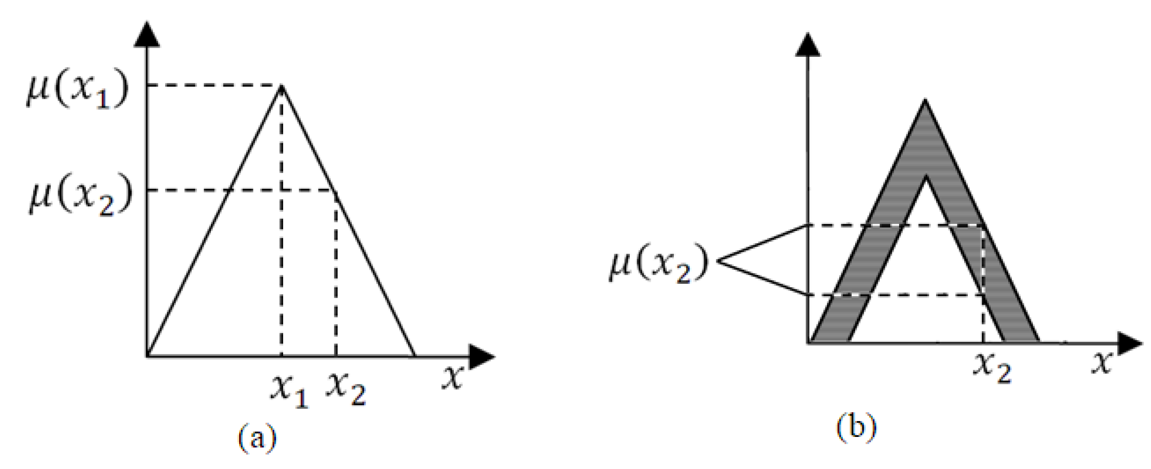
2.4. Fuzzy Time Series Models of Higher Orders

Prediction is made by using a variety of methods and approaches [30]. If the deterministic model of the system is absence then such methods based on the study of the evolutionary history of processes and indicators. One of the popular tools for studying the evolutionary history of processes and indicators are time series models. Time series models have a different nature: statistical, based on neural networks, fuzzy, etc. The use of models is complicated by data characteristics. Data may require preprocessing, normalization, may have a high degree of uncertainty.
The nature of the fuzzy time series is caused by using expert evaluations. Expert evaluations have a high level of uncertainty and fuzziness. Fuzziness, unlike stochastic uncertainty, makes it difficult or impossible to use statistical methods and models. However, fuzziness can be used to make subject-oriented decisions based on approximate reasoning of an expert. The formalization of intellectual operations that simulate fuzzy human statements about the state and behavior of a complex system nowadays forms an independent area of scientific and applied research called “fuzzy modeling” [31].
First-order sets (type 1) are usually used to build a process model. Type 1 fuzzy sets are used to represent or to create a model of domain uncertainties [32].
L. A. Zade introduced in 1975 second-order fuzzy sets (type 2) and higher-order fuzzy sets (type n) to eliminate the shortcomings of type 1 fuzzy sets [33]. The main disadvantage is the mapping of the membership function to exact real numbers. The solution to this problem can be the use of type 2 fuzzy sets, in which the boundaries of the membership regions are themselves fuzzy [32]. For each value of the x variable from the universe X the value itself is a function, not a value at a point. This function represents a type-2 fuzzy set, which is three-dimensional, and the third dimension itself adds a new degree of freedom for handling uncertainties.
The union, intersection, and complement operations can be over type 2 fuzzy sets. Type 2 fuzzy sets have an extended representation of uncertainties, which creates additional computational complexity.
The designation of the fuzzy type 2 membership function can graphically shown as a region called the footprint of uncertainty (see Figure 2). In comparison to using the membership function with crisp boundaries, the values of the type 2 membership function are themselves fuzzy functions.
This approach has given an advantage in bringing the fuzzy model closer to the model in linguistic form. People may have different evaluations of the same uncertainty. There was a need to exclude an unambiguous comparison of the obtained value of the degree of membership function. Thus, the risk of error accumulation is reduced when an expert sets the membership degrees due to not including points located near the boundaries of the function and being in uncertainty.
Blurring boundaries is the first step in moving from type 1 fuzzy sets to type 2 fuzzy sets. It is required to choose the type of membership function at the second step as is done for type 1 fuzzy sets (for example, triangles).
The uncertainty present in the tasks of managing the activities of any enterprise and characterized by the statements of experts containing incomplete information, with fuzzy and unclear information about the main parameters and conditions of the analyzed problem. Thus, the solution to the control problem becomes complicated and is generated by multiple factors. The combination of these factors in practice creates a wide range of different types of uncertainty. Therefore, it becomes necessary to use methods that allow the use of blurry values of indicators.

A Time Series Model Based on Fuzzy Sets of Type 2

Type 2 fuzzy sets A ˜ in the universum U can be defined using type 2 membership function. Type 2 fuzzy sets can be represented as:
A ˜ = ( ( x , u ) , μ A ˜ ( x , u ) ) | x U , u J x [ 0 , 1 ] ,
where x U and u J x [ 0 , 1 ] in which 0 μ A ˜ ( x , u ) 1 . The main membership function is in the range from 0 to 1, so the appearance of the fuzzy set is expressed as:
A ˜ = x U u J x μ A ˜ ( x , u ) / ( x , u ) J x [ 0 , 1 ] ,
where the operator denotes the union over all incoming x and u.
Time series modeling needs to define interval fuzzy sets and their shape. Figure 2 shows the appearance of the sets.
Triangular fuzzy sets are defined as follows:
A ˜ i = ( A ˜ i U , A ˜ i L ) = = ( ( a i 1 u , a i 2 u , a i 3 u , h ( A ˜ i U ) ) , ( a i 1 l , a i 2 l , a i 3 l , h ( A ˜ i l ) ) ) .
where A ˜ i U and A ˜ i L is a triangular type 1 fuzzy sets; a i 1 u , a i 2 u , a i 3 u , a i 1 l , a i 2 l , a i 3 l , is reference points of type 2 interval fuzzy set A ˜ i ; h is the value of the membership function of the element a i (for the upper and lower membership functions, respectively).
An operation of combining fuzzy sets of type 2 is required when working with a rule base based on the values of a time series. The combining operation defined as follows:
A ˜ 1 A ˜ 2 = ( A ˜ 1 U , A ˜ 1 L ) ( A ˜ 2 U , A ˜ 2 L ) = = ( ( a 11 u + a 21 u , a 12 u + a 22 u , a 13 u + a 23 u ; m i n ( h 1 ( A ˜ 1 U ) , h 1 ( A ˜ 2 U ) A ˜ 1 U ) ) , m i n ( h 2 ( A ˜ 1 U ) , h 2 ( A ˜ 2 U ) ) , ) ; ( a 11 l + a 21 l , a 12 l + a 22 l , a 13 l + a 23 l ; m i n ( h 1 ( A ˜ 1 L ) , h 1 ( A ˜ 2 L ) ) , m i n ( h 2 ( A ˜ 1 L ) , h 2 ( A ˜ 2 L ) ) ) .

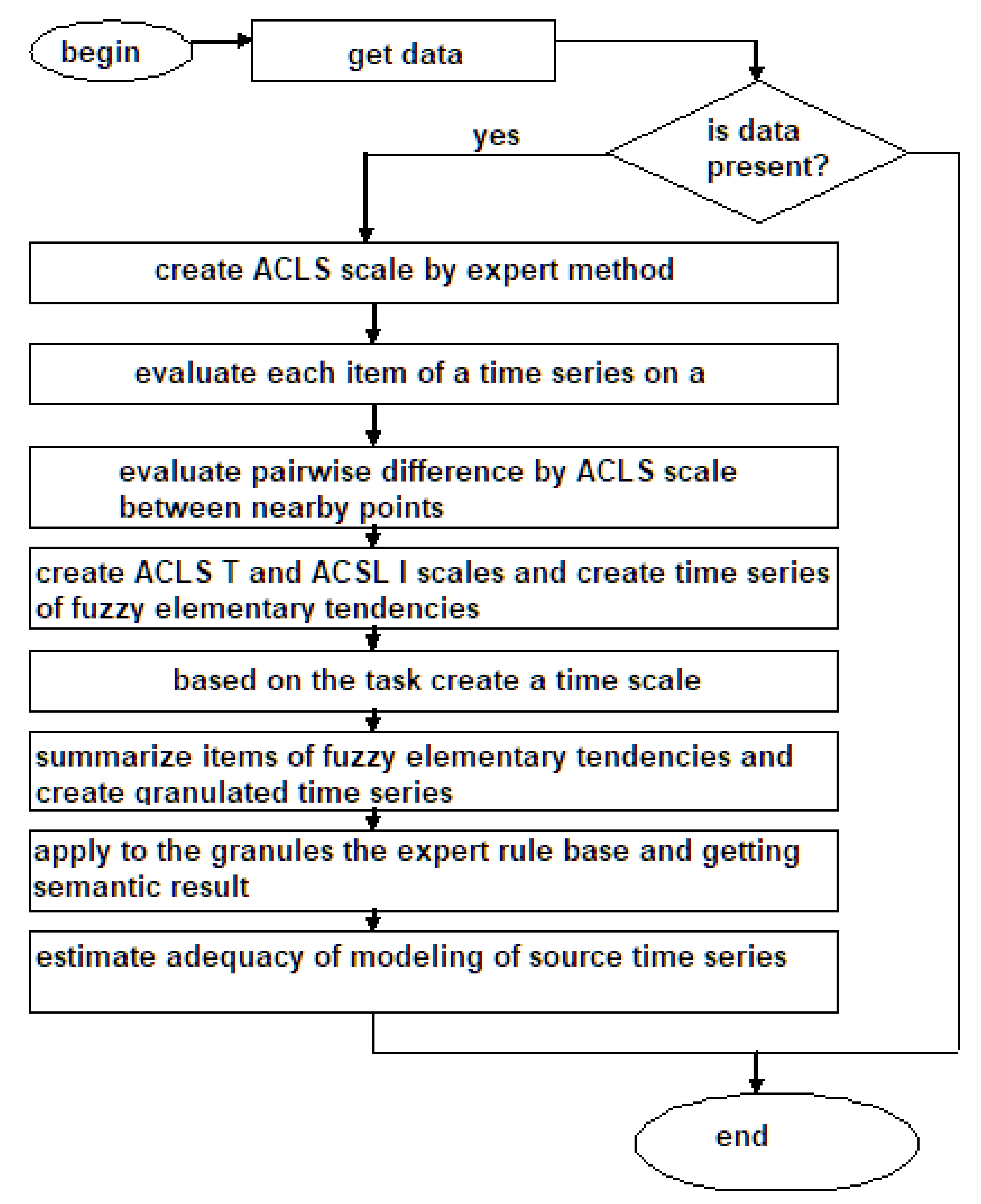
2.5. Algorithm for Smoothing and Forecasting of Time Series

The main principle of the proposed algorithm is closely related to the nature of the time series. Type 2 fuzzy sets are used for modeling in the process of smoothing and forecasting of time series because the time series has the interval nature [32].
The proposed algorithm can be represented as a sequence of the following steps:
  • Determination of the universe of observations. U = [ U m i n , U m a x ] , where U m i n and U m a x are minimal and maximal values of a time series respectively.
  • Definition of membership functions for a time series M = { μ 1 , , μ l } , l n , where l is the number of membership functions of fuzzy sets; n is the length of a time series. The number of membership functions and, accordingly, the number of fuzzy sets is chosen relatively small. The motivation for this solution is the multi-level approach to modeling a time series. It is advantageous to reduce the number of fuzzy sets at each level to decrease the dimension of the set of relations. Obviously, this approach will decrease the quality of approximation of a time series. However, creating the set of membership functions at the second and higher levels will increase the approximation accuracy with an increase in the number of levels.
  • Definition of fuzzy sets for a series. In that case, the superscript defines the type of fuzzy sets. A 1 = { A 1 1 , , A l 1 } , A 2 = { A 1 2 , , A m 2 } , where l is the number of type 1 fuzzy sets, m is the number of type 2 fuzzy sets.
  • Fuzzification of a time series by type 1 sets. x i y ˜ i = F u z z y ( x i )
  • Fuzzification a time series by type 2 sets.
  • Creation of relations. The rules for the creation of relations are represented in the form of pairs of fuzzy sets in terms of antecedents and consequents, for example: A 1 1 A 1 2 A 2 1 A 2 1 .
  • Doing forecasting for the first and second levels based on a set of rules. The forecast is calculated by the centroid method, first on type 1 fuzzy sets A 1 = { A 1 1 , , A l 1 } , then on type 2 fuzzy sets.
  • Evaluation of forecasting errors.
The amount of fuzzy sets of each type in the operation of the described algorithm is hard to extract from an integral time series. The brute force of quantities of fuzzy sets is also expensive. The main purpose of using fuzzy sets of higher orders is a high degree of approximation of modeling objects. The best method to select the number of fuzzy sets is to obtain information from outside of the time series, for example, based on rules generated by machine learning methods or by an expert.
The general steps of the time series analysis algorithm are presented in Figure 3.

3. Applied Problems of Time Series Modeling

3.1. Problems Statement of Applied Time Series Modeling

Technology, economics, and other various subject areas can be objects of time series modeling. Predicting the behavior of objects, and identifying key indicators for objects of a subject area is the main purpose of time series modeling.
The efficiency of aviation use in the expected operating conditions is dependent on ensuring a high level of flight safety. The safety of flights depends on many factors, such as the reliability of the aircraft, the systems that ensure the aircraft functioning, operational mode, human factor, and adverse factors. Some factors cannot be predicted and their effect on the flight process can not be changed. However, some factors allow forecasting to reduce their negative impact. One of the predicted factors affecting flight safety is airplane equipment failure. The reliability of the aircraft units is checked during technical inspection. However, it is necessary to control the condition of the aircraft units between inspections too. Expert analysis of time series of key indicators can be used to diagnostics of aircraft equipment units. The principal attention must be given to dangerous trends in indicators. It is possible to create a tool used to diagnose aircraft units between technical inspections to improve the expert’s work. This tool is based on formalized expert knowledge, and its purpose is to identify potentially defective aircraft equipment units [34].
Usually, the technical system condition is described by a combination of some parameters characterizing an object. Thus, the behavior of an object as a change of values of its key indicators in time can be represented by time series. Therefore, modeling and predicting the behavior of an object can be done through analysis of the time series of its indicators. Trends in long-term growth (recession) or long-term stability of some indicator may be dangerous if its value is large or too small. All data about the normative behavior of the object and the duration of the tendencies persistence are expressed in linguistic form. Modern intelligent methods of time series analyzing are based on the information granules definition. The listed features of aircraft diagnostics determine the relevance of mathematical modeling and analyzing of the behavior of aircraft units based on the analysis of granular time series [34].

3.2. Diagnostics of the Technical System

Currently, all aircrafts are equipped with monitoring systems of their technical condition. Equipment failures and the human factor are the two main factors that can be controlled to reduce their negative impact. The human factor arises from an incorrect assessment of the situation as a result of equipment failures. Let us take a closer look to the problem of diagnosing the technical condition of a helicopter to determine the probability of equipment failure.
Only serviceable helicopter are used for flights. A serviceable object is in a condition in which it corresponds to all requirements of design and technical documentation. However, there is a more complete classification of helicopter conditions. For example, the working condition includes operational and idle state. The object is not used for its intended purpose in an idle state and can be in (see Figure 4):
  • The storage state;
  • The planned idle state;
  • The internal idle state (the failure or incompleteness of the scheduled maintenance);
  • The external idle state (different organizational reasons).
All helicopter malfunctions can be divided into two categories: damage and failure.
Damage is a violation of the serviceable condition of an object when it is in an operational state. The severity of the damage is divided into significant and non-significant. Non-significant damages may result in aircraft failure.
The operational state of the helicopter is characterized by a combination of several technical indicators. The failure can occur when the value of some of these indicators goes beyond the permissible limits.
All helicopter failures can be divided into two groups by reliability theory [6]:
  • Failures as a result of defects in design, operational documentation, production technology;
  • Failures as a result of the dispersion of units characteristics within the established permissible values, or as a random adverse combination of operating modes.
Helicopter failures can be classified as follows:
  • For reasons of occurrence of failures:
    • Design failures. Design failures arise due to errors in the design of the product, inaccurate consideration of the actual operating conditions of the product, etc.;
    • Production failures. Production failures arise due to deviations in the technological process of the product, improperly organized metrological support of production processes, etc.;
    • Operational failures. Operational failures usually occur due to violation of the conditions of the established operating modes of products.
  • By the nature of the change in the quality indicator of the helicopter [6]:
    • Sudden failures. Sudden failures characterized by a sudden change in one or more properties of the helicopter;
    • Gradual failures. Gradual failures are characterized by a gradual (slow) change in the values of one or more parameters of the helicopter. The causes of gradual failures of helicopter include:
      The aging process of structural elements as a gradual change in the properties of materials over time;
      Helicopter wear. Wear is a process of gradual change of material during friction. Wear occurs when the material particles are separated from the interaction surface of the material with their subsequent permanent deformation.
      Fatigue process of structural elements. Fatigue of elements is the process of the gradual accumulation of material damage under the influence of alternating mechanical stresses. Fatigue of elements can be thermal and mechanical.
  • By the nature of the stability of a failure state:
    • Persistent failures;
    • Glitches;
    • Intermittent failures.
  • By the possibility of following use of the helicopter:
    • Complete failures—loss of all product features;
    • Partial failures—when the product can still perform some functions declared in the functional specification.
  • By the presence of external manifestations of failure:
    • Overt failure;
    • Hidden failure.
  • By possibility and advisability of the failure elimination:
    • Removable failures;
    • Fatal failures.
  • By mutual dependence from each other failures are divided into:
    • Independent failures have their reasons for occurrence;
    • Dependent failures due to failure of another unit.
  • By the degree of impact on flight safety:
    • Catastrophic failures;
    • Emergency failures;
    • Failures leading to a difficult situation;
    • Failures that complicate the conditions for further flight.
  • By the nature of detection using information-measuring control:
    • Controlled failure;
    • Uncontrolled failure.
The helicopter contains about 50 different mechanical components and units with a limited resource predisposed to failure. Monitoring all of these units is impractical and impossible, so we need to highlight the main ones.
The next central units require additional control over their condition during operation:
  • Main gearbox;
  • Engine power plant.
The main gearbox is designed to transmit torque from the engines to the main rotor of the helicopter and to drive units mounted on the gearbox. The gearbox consists of the following main parts: main rotor shaft drive, main rotor shaft, tail rotor drive and unit drives, crankcase, two freewheels, three magnetic plugs, and oil sight glasses. The lubrication system of the main gearbox provides the supply of pressurized oil to the bearings and gears, their lubrication, cooling, and removal of wear products from the gearbox [6].
The power plant of the helicopter includes two turboshaft engines. A feature of the engine design is the presence of a free turbine kinematically not connected with the rotor of the turbocharger of the engine. The engine consists of the following components: drives of auxiliary devices, fuel system, axial compressor, combustion chamber, exhaust device, air intake system, starting system [6].
List of failures and the physical indicators that accompany them can be distinguished for these elements [6].
If we observe the state of the main gearbox, then we can track the destruction or wear of the oil filter and its parts and units by the temperature and pressure of the oil [6].
The following failures can be added to the list of monitored power plant failures:
  • Destruction or wear of parts and components of a free turbine;
  • Non-localized engine destruction;
  • Starter failure;
  • Engine shutdown;
  • Destruction or wear of parts and units of a turbocharger;
  • Destruction of the engine oil unit.
These failures are associated with the readings of the following physical indicators: torque, exhaust temperature, inlet oil temperature, oil pressure.
Thus, we see that the state of the system is characterized by indications of certain physical indicators that can be measured using various kinds of sensors, which are usually equipped with helicopters. The values of these indicators must be within acceptable limits with the correct operation of the system. If the value of some indicator goes beyond these boundaries or if its value is near one of the boundaries and a steady increase (or decrease), this can indicate a dangerous situation during the further operation of some element. Table 1 presents a list of physical indicators with normative indicators that make it possible to evaluate the state of some element [6].
Helicopter units have a limited resource and operated until resources are not reached some state of using. Helicopter units are replaced or inspected by schedule when this state is reached. However, equipment failure may occur before scheduled maintenance. One of the solutions to this problem may be to increase the frequency of helicopter technical inspections. However, often this option is not economically viable. Therefore, a cheaper and more efficient method is needed.
A technical inspection of a helicopter is an expert’s diagnostics of its units to establish its serviceability and possible operation. Because conducting a very frequent technical inspection is not economically viable, a cheaper solution to this problem would be to use an expert system to conduct equipment diagnostics. Such inspection can be done on a pre-flight run of the engine, or in the process of analyzing data collected after a helicopter flight. It is required to evaluate the values of key physical indicators and their trends as a result of the analysis. The main task is to evaluate the danger of the value and tendency of a particular indicator. The presence of dangerous values and trends may indicate that the unit is behaving incorrectly and, perhaps, it is not worth releasing the board on a flight or making the decision to inspect the helicopter again [34].
It is also necessary to analyze the data to identify the residual resource of the unit. In this case, the data will be analyzed not only for a single flight, but also to a history of several flights. In the framework of this study, we will focus on the problem of evaluating the correctness of the behavior of the main gearbox and the engine power plant according to flight data. It is necessary to build models of the behavior of these units and get appropriate conclusions using these models. We will build models in the form of the base of expert evaluations about the behavior of a particular unit.
Let us see the power plant of the engine and the main gearbox in the form of the next system S = ( A , B , C , D ) . For engine power plant A = {Engine Torque, Exhaust Temperature, Oil Pressure, Oil Temperature}. For main gearbox A = {Oil Temperature, Oil Pressure}. Table 2 presents expert evaluations for each indicator [34].
The algorithm of expert evaluation of the helicopter units is shown in Figure 5.
Two static simplified scales, one static full scale, and one combined simplified scale are used in this work. Static Simplified Scales: Intensity Scale (ACLSI) and Duration Scale (Time). Dynamic Scale: Linguistic Grade Level Scale (ACLS). Combined Simplified Scale: Trending Scale (ACLST).
ACLS scale has a basic term set: {“Dangerously Low”, “Low”, “Normal”, “High”, “Dangerously High”}. The type of membership functions (cluster or basic) and its parameters are determined dynamically.
The ACLSI scale has a basic term set: {“Low”, “Medium”, “High”}. The type of membership function is basic. The power of the set is 3, and the parameters are:
  • “Low”: (0.25, 0.5, 1.9);
  • “Medium”: (1.6, 2.5, 3.45);
  • “High”: (3.06, 4, 5);
The ACLST scale has a basic term set: {“Recession”, “Stability”, “Growth”}. The type of membership function is basic. Membership function parameters are determined based on the RTend and TTend ACLS operations:
  • “Recession”: (minZ-1, minZ, −0.45), where minZ is the minimum value of the difference obtained on the analyzed series;
  • “Stability”: (−0.5, 0, 0.5);
  • “Growth”: (0.45, maxZ, maxZ+1), where maxZ is the maximum value of the difference obtained on the analyzed series.
The time scale depends on the nature of the analyzed series. Different time intervals will be significant for different series. Therefore, the construction of this scale, the choice of the type and the selection of the parameters of its membership functions are fully expert. The time scale has a basic term set: {Short, Average, Long}. Time is measured in seconds. Membership function parameters are:
  • “Short”: ( a < 0 , b = 0 , c = 5 );
  • “Average”: ( a = 4 , b = 6 , c = 10 );
  • “Long”: ( a = 9 , b = 14 , c > 16 ).
Now we need to determine the rules for evaluating the unit state. We use the following concepts to evaluate the situation O = {Normal, Possibly Dangerous, Dangerous}.
Then, the parameters B and C for any value: G 1 = {“Long-term stability”} or G 2 = {“Average stability”} with the value “Dangerously Low” or “Dangerously High”. Frequent appearance of granules G 3 = {“Short intense growth”} or G 4 = {“Short intense recession”} at a value of “Normal” or G 5 = {“Short small growth”} at a value of “High” or G 6 = {“Short small recession”} at a value of “Low” [34].
The right part of the rules characterizes the level of danger D: G1 -> “Dangerous”, G2,G3,G4,G5,G6 -> “Possibly Dangerous”.
Thus, the task of analyzing the technical series is reduced to the task of interpreting the data of the physical indicators based on the rules to diagnose helicopter units, such as the main gearbox and engine power plant. Diagnostics is a sequence of the following steps:
  • Getting information about the values of key physical indicators.
  • Formation of a time series for each of these indicators.
  • Formation of a granular time series.
  • Evaluation of the state of the helicopter. A condition is considered correct if none of the values fell into a dangerous situation.
  • If the work is recognized as not correct for less than 20% of the values, then repeated testing is necessary. Otherwise, it is necessary to conduct a technical inspection of the problem unit.

3.3. Forecasting Technical Time Series

The development of computer networks (CN) of various levels (from local to global data transmission networks) in the last decade has led to an increase in the integration of data networks with production processes (commercial activities). The work of enterprises is increasingly dependent on the quality of service in networks. This task cannot be accomplished without analyzing the CN-Business-Process system and predicting the development of this system. This requires modeling of computer networks at the design stage and also modeling of the existing computer networks [35].
The relevance of this problem is due to the complexity of the architecture of computer networks. Testing network performance comes down to measuring the parameters of QoS (Quality of Service) or network performance (NP) for various values of the parameters of the incoming traffic load of the network [35].
One of the modeling tasks is to analyze the throughput of a computer network (traffic, load, delay, etc.). The network nodes act as generators and traffic handlers. If for switching equipment many libraries allow performing simulation, then it is necessary to implement models in each specific simulation case for user nodes.
The indicated CN parameters form the time series. The values of the obtained time series are conveniently interpreted for experts in terms of expert estimates of the dynamics of changes in productivity: growth, recession, downtime, etc. Periodic or regular monitoring of the volume of traffic and protocols is one of the most important tasks of operational network support. Such monitoring allows:
  • To detect errors not detected at the testing stages;
  • To detect unauthorized access to resources from individual users;
  • To optimize network configuration;
  • To balance the load between its resources;
  • To provide network development planning.
The dynamics of the time series of the traffic of computer networks depends on the observation time intervals and can be characterized by a high degree of uncertainty due to the heterogeneity of behavior in the form of a combination of unsteady and stationary behavior. The unsteady behavior of such time series is also heterogeneous. This creates some difficulties in the selection of statistical and neural network models [35].
The analytical form of the identified dependence requires a complex process of qualitative interpretation in terms that are understandable to network administrators or expert systems. The values of the time series have an additional character in the form of an expert assessment for a specialist expert. Therefore, the assessment of the effectiveness of the functioning of networks in practice is more often determined expertly based on the rules that operate with the qualitative concepts of “increase”, “decrease”, “below the critical level”, “above the critical level”, etc. [35].
It was possible to generate expert estimates in the process of construction models and to get ready-made linguistic interpretations of the results about expected short-term trends using the methodology of the structural-linguistic approach, as well as a description of the main trend for a given section of the network traffic [17,35].

3.4. Forecasting Economic Time Series

The task of analyzing economic time series can be formulated as the task of financial analysis of an enterprise. The central target audience for such an analysis are small and medium-sized enterprises. Adequate analysis and forecast of trends in changes of economic indicators are important for them for the following reasons [36].
First of all, this approach avoids mistakes in managerial decisions and more effectively allocates resources, which small enterprises usually do not have so many [36].
Secondly, expensive services of consulting firms for express analysis are not available for small and medium-sized enterprises. Therefore, they focus on the use of specialized or universal software products. The use of statistical packages (Statistica, SPSS, etc.) for the operational analysis and forecasting the time series of economic indicators, in addition to the high cost of a license, requires highly qualified managers in the field of mathematical statistics and significant intellectual and time costs due to the complexity and variety of models and time series processing methods. Reducing material costs, including staff training, the acquisition, updating of hardware and software, is no less relevant for small and medium enterprises, especially in an unstable economy, which creates the requirement for low-cost software products [36].
The task of assessing the financial statement of the enterprise can be divided into several subtasks. It is necessary to highlight several indicators characterizing the financial condition of the enterprise and determine the methodology for their calculation and the rules for the economic evaluation of their values and trends. A list of some of the metrics used is provided in the Table 3. The calculation formulas indicate the lines from the regulated financial statements [36].
It is necessary to form a time series characterizing each of the selected indicators and identify the general trend of each series. You need to take the financial statements of the enterprise for several periods and recalculate the indicators using the available formulas to do this.
It is also important to give an economic assessment of the current state of affairs at the enterprise, using the generated set of rules for indicators. Each indicator has a certain characteristic of its dynamics, and some indicators are also characterized by normative values from an economic point of view. For example, an increase in the coefficient value current liquidity is considered favorable, a decrease is an opposite. However, the norm for the value of this indicator is a segment from 1 to 2. If the value of the indicator is less than one, then they say about the danger of this situation, since the enterprise is considered insolvent, due to the fact that working capital is not enough to cover short-term obligations. If the value of the indicator is more than 2, then this situation is considered undesirable, since it is possible for the enterprise to invest its funds irrationally and their use is inefficient. Thus, you can give an economic assessment of the current state of the enterprise having a similar type of rule for each indicator [37].
Furthermore, it is necessary to analyze the existing one and predict the future trend of each indicator and give an economic interpretation of this forecast. The necessity and relevance of this subtask is a matter of course. It is clear that in order to make a competent managerial decision it is necessary not only to know how things are at the current moment but also what dynamics should be expected in the future [37].
In this case, the input is the time series of the selected economic indicators, the output is the predicted and recorded trends in their development, as well as their semantic interpretation.
The ACLS scale has a basic term set: {“Low”, “Below Average”, “Middle”, “Above Average”, “High”}. The type of membership functions (cluster or basic), as well as its parameters are determined dynamically. For the task of analyzing economic series, the ACLT and ACLI scales are the same as described above.
The time scale can have a basic term set: {“Very Short”, “Short”, “Long”, “Very Long” }. Type of membership functions is basic. The parameters of membership functions are determined based on the distance between the points of the analyzed time series on the time scale and are expressed in months. Membership function parameters are:
  • “Very Short”: (0, 3, 5);
  • “Short”: (4, 6, 8);
  • “Continuous”: (7, 9, 11);
  • “Long”: (10, 12, 14);
  • “Very Long”: (13, 15, 27).
The expert knowledge base will contain the following rules:
  • For current ratio:
    • “If long-term growth is observed, then the favorable situation at the enterprise”;
    • “If a long or medium decline is observed, then the unfavorable situation at the enterprise”;
    • “If a short intense decline is observed, then the company needs to be more careful about its cash and assets”.
  • For quick ratio:
    • “If there is continued growth, then the favorable situation at the enterprise”.
  • For the coefficient of financial independence:
    • “If long-term growth is observed, then the favorable situation at the enterprise”;
    • “If a long or medium decline is observed, then the unfavorable situation at the enterprise”.
  • For the coefficient of financial independence in terms of working capital:
    • “If long-term growth is observed, then the favorable situation at the enterprise”;
    • “If a long or medium decline is observed, then the unfavorable situation at the enterprise”.
  • For the financial independence ratio in terms of stocks:
    • “If long-term growth is observed, then the favorable situation at the enterprise”;
    • “If a long or medium decline is observed, then the unfavorable situation at the enterprise”.
  • For the coefficient of attraction (ratio of own and borrowed funds):
    • “If long-term growth is observed, then the favorable situation at the enterprise”;
    • “If a long or medium decline is observed, then the unfavorable situation at the enterprise”.
In this case, the task of analyzing economic time series is reduced to the task of forecasting and interpreting the trends of key indicators. It is necessary to smooth the time series, because the trend of indicators is of interest.

4. Experiemts

It needs to do experiments with different types of time series such as technical and economic, to evaluate the effectiveness of the developed models.
The effectiveness of this method can be assessed when solving the problem of modeling the behavior of the main gearbox and the power plant of the helicopter engine for technical series. The system must correctly diagnose possible defects or report their absence. Therefore, it is necessary to analyze the data characterizing machines without defects and with alleged defects, and then determine the number of cases in which the system gave incorrect information. We will consider the system to be effective only if the error does not exceed 9% [6].
It is necessary to evaluate the application of the developed models in the task of analyzing the financial results of the enterprise for the economic series.
The efficiency of using the module, in this case, can be evaluated by several criteria. It is also necessary to evaluate how well models predict trends in indicators and the values themselves. The SMAPE criterion is used as a criterion for the quality of prediction of indicator values. We will consider the forecast to be good if the average SMAPE for all series of the experiment does not exceed 20%.

4.1. Characterization of the Service for Technical Series Modeling

Data were taken on the run of three machines and data was generated simulating certain defects for the experiment. Description of the rows is given in Table 4.

4.2. Characterization the Database for Economic Time Series Modeling

The service database contains the set of time series. They are characterized by size, character, and origin. The description of the rows is given in Table 5:

4.3. Technical Series Experiment Results

The results of experiments with data of Table 4 are given in Table 6.
We can conclude that the system recognizes dangerous situations according to the results of the experiments.

4.4. The Results of Experiments with Economic Time Series

Several experiments were carried out with 11 time series (see Table 5).
Experiment 1. Comparison of forecast quality using F-transform and fuzzy tendency (Table 7).
The fuzzy tendencies method gives better forecast quality indicators in comparison to the F-transform method, but worse than the integrated technique. The method demonstrates the best performance with a short time series.
Experiment 2. Comparison of forecast quality by applying uniform partitioning and clustering of a fuzzy set of a time interval of time series. Table 8 shows the results of 50 experiments with time series of economic indicators. The purpose of the experiments is evaluation of the forecast quality using the cluster method of partitioning and the method of uniform partitioning. The cells with the smallest SMAPE for the cluster partition are marked by the bold font in Table 8.
The average forecast error for cluster partitioning is 6.48%. The average forecast error for uniform partitioning is 12.54%. The total average error for both methods is 9.15%. The experiment shows the following conclusions. Firstly, the average error does not exceed 20%, which is acceptable for the fuzzy time series. Secondly, the cluster partitioning method often gives a better result than the uniform partitioning. Thirdly, the average error of the cluster method of partitioning is less than the error of the uniform method about two times.

4.5. Benchmarking Efficiency

A comparison of the effectiveness of the methods was carried out with the results of the forecasting competition NNG. Time series were selected for which forecasting qualities are known.
The time series was selected to test the method from the competition NN GC1 No. 102 from the dataset: http://www.neural-forecasting-competition.com/downloads/NN3/datasets/NN3_COMPLETE.xls.
The time series has a length of 126 points. A forecast of 18 points in the time series and 5 trend points. The following configuration of the method parameters was selected based on the results of enumerating all the parameters and calculating the forecast on the test part of the time series:
  • Trend forecasting method: neural network with absolute values;
  • The degree of autoregressive by trend points: 3;
  • Number of points covered by the basis function: 11.
In this case, the SMAPE estimates 26.06% were obtained for the trend, for the time series is 18.88%. The figure shows the forecast for the test part of the time series for the best configuration of the method.
Trend forecast (Figure 6):
Time series forecast (Figure 7):
The time series was selected to test the method from the competition NN GC1 No. 108: the time series has a length of 115 points. A forecast of 19 points in the time series and 5 trend points. The following configuration of the method parameters was selected based on the results of enumerating all the parameters and calculating the forecast on the test part of the time series:
  • Trend forecasting method: neural network with absolute and relative values;
  • The level of autoregressive by trend points: 1;
  • The number of points covered by the basis function: 9.
The following SMAPE estimates 24.76% were obtained for the trend, for the time series is 15.008%. The figure shows the forecast for the test part of the time series for the best configuration of the method. Trend forecast (Figure 8):
Time series forecast (Figure 9):
Table 9 shows a comparison of the forecast results of the proposed method and the methods whose results are available on the competition website NN3.

4.6. Analyzing Time Series of Economic Indicators

Analysis of the activities of any enterprise is based on the study and evaluation of the values and dynamics of economic indicators, which are formed according to the financial statements [38].
The most important indicators characterizing the activities of the enterprise are considered, first of all, financial indicators. It is the financial condition of the enterprise that determines its competitiveness, its potential in business cooperation, and makes it possible to assess the degree of guaranteeing the economic interests of both the enterprise itself and its partners in financial and commercial relations [38].
Experiment 1. 12 real time series of a short length of technical and economic indicators of an individual organization were used to compare the proposed model of fuzzy trends with optimal statistical models constructed by the control algorithm in the ForecastPro software based on the method of complexing models that include trend, stochastic ARIMA-models and models of the exponential smoothing class [38].
It was decided to smooth them out first using the F-transform method to apply the method for predicting a fuzzy elementary tendency of the structural-linguistic approach [38].
The results presented in Table 10, show that the proposed model of fuzzy tendency for the studied time series of technical and economic indicators on average generates a more accurate forecast, not only in comparison with the basic fuzzy and neural network models but also in comparison with the optimal models chosen by the manager algorithm in the ForecastPro [38].
Experiment 2. 20 real technical and economic time series of short lengths were used to compare fuzzy trend models with statistical models like ARIMA 35%. Time series did not have enough values to build an ARIMA class model, so the time series were divided into two groups: a comparison with ARIMA models was carried out for 65% time series. The obtained indicators of forecasting accuracy of the base models of various approaches are given in Table 11.

4.7. Analyzing Time Series of Computer Network Traffic

Let see the quantifying the effectiveness of a fuzzy model and a method for predicting trends in solving problems of short-term forecasting of time series of telecommunication traffic (Figure 10) in a computer network in comparison with fuzzy and neural models. The results obtained in the developed software are presented in Table 12.
An analysis of the use of fuzzy modeling methods for trends in the tasks of short-term forecasting of computer network traffic has established that all identified models are adequate [38].
The test results of three fuzzy models and one neural network model presented in Table 12. In total, 15 experiments of short-term forecasting of the traffic of the computer network indicate the usefulness and prospects of using fuzzy trending for these purposes [38].
  • Fuzzy models of the proposed structural-linguistic approach demonstrate a stable advantage to the compared basic fuzzy model and one neural network model. This is confirmed by the fact that models of fuzzy trends:
    (a)
    Are adequate in solving all problems (100%);
    (b)
    Surpasses the fuzzy model in the accuracy of forecasting the values of the time series in all problems (100%) and on average more than 2.5 times;
    (c)
    Is superior or not inferior to the fuzzy model in the accuracy of predicting fuzzy trends in the time series in all tasks (100%);
    (d)
    Surpass neural network models in 80% of tasks in the accuracy of forecasting the values of the time series and on average more than three times;
    (e)
    More than two times the accuracy of predicting fuzzy trends in the time series;
    (f)
    Is inferior in 20% (in three tasks) in the accuracy of forecasting the values of the time series by 1.3 times in neural network models.
  • Neural network models are inadequate in solving one problem (in 6%).
  • The fuzzy model in 94% of tasks is inadequate (in 14 out of 15 tasks), significantly inferior in the accuracy of forecasting the values and trends of the time series to the author’s models of fuzzy trends (more than 10 and six times, respectively).
  • The fuzzy model in 47% of the tasks is inadequate (in seven out of 15 tasks), significantly inferior in the accuracy of forecasting the values and trends of the time series to the author’s models of fuzzy trends (more than 2.5 and five times, respectively).
The results obtained indicate the competitiveness of the structural-linguistic approach in comparison with the basic well-known analogs of fuzzy and neural network modeling.
The study of the author’s models of fuzzy trends in the efficiency of forecasting values on the time series of the traffic of computer networks depending on the length of the time series and the forecast horizon allows us to draw the following conclusions [38]:
  • For short time series (25 and 55 values) the accuracy of forecasting the values of the time series according to the SMAPE criterion is acceptable and stable (from 2.5% to 6.6% and from 8.7% to 15%, respectively);
  • For a smooth long time series prediction accuracy of time series values according to the SMAPE criterion is low, while it is 3 times higher for the forecast horizon from 2% to 10% and 1.4 times lower for the forecast horizon of 20% compared with the undeveloped time series.
  • As the length of the time series increases, the accuracy of predicting the values of the time series decreases on average, and the error increases.
In the short-term forecasting of the time series of telecommunication traffic with a length of 190 values, the potential of fuzzy models is shown (fuzzy model SMAPE is 67.8%; model of fuzzy trends SMAPE is 83.7%) compared with the results of using the stochastic model ARIMA (1,0,1) SMAPE is 190.7%.

4.8. Smoothing and Predicting Time Series Based on Type 2 Fuzzy Sets

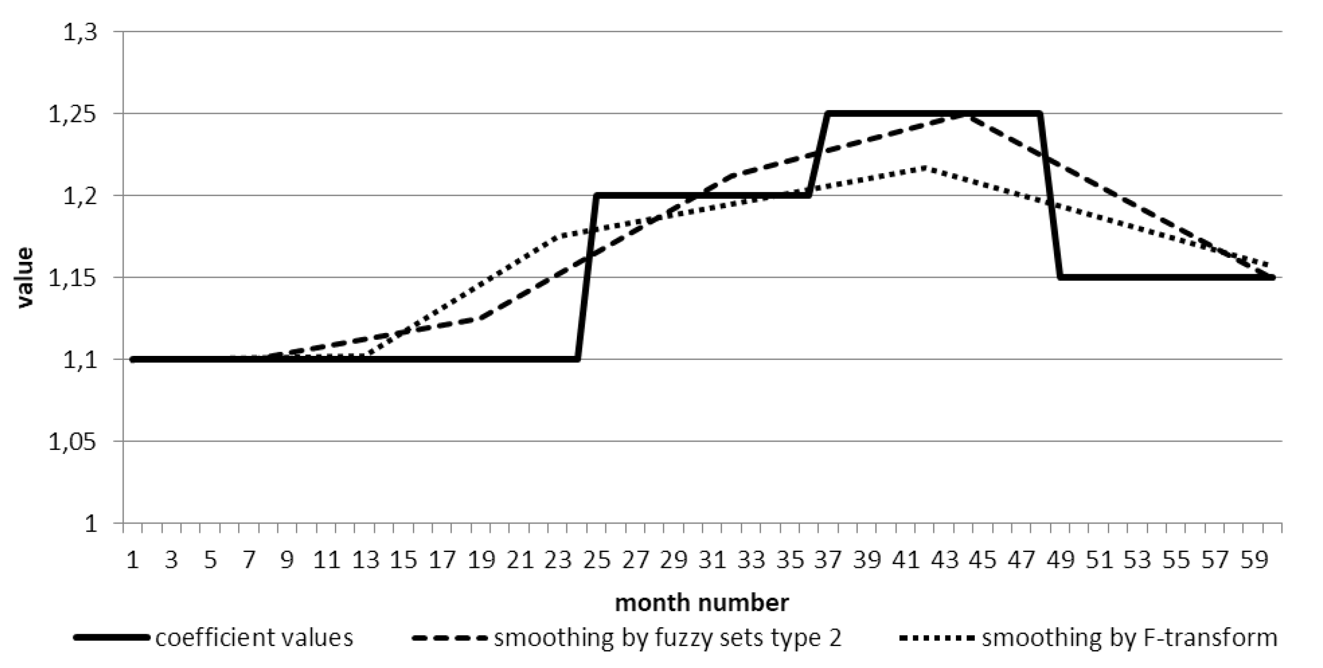
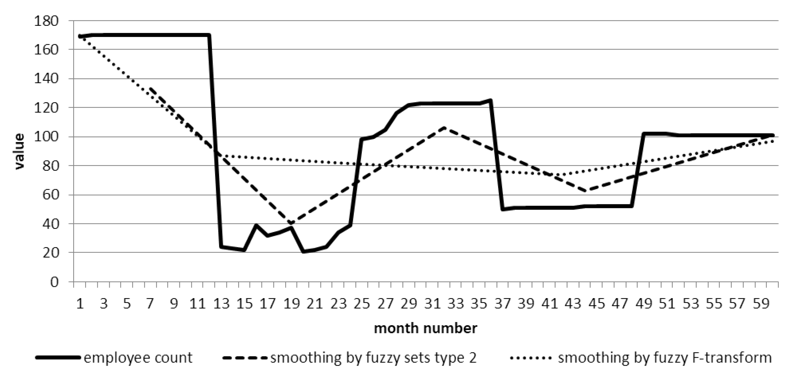
4.8.1. Time Series Smoothing

Consider the process of smoothing the coefficient. The original time series has 60 points. In the graph of Figure 11 shows the smoothing of the time series by the F-transform method for comparison.
The set of 15 fuzzy sets of type 2 and 5 sets of type 1 was selected for smoothing. This choice is argued by the fact what for this time series it was important to get one of the consequences in the dynamics of the number of employees: very high, high, medium, small, and very few. The second level of fuzzy sets allows you to get a model of the uncertainty of belonging to one of the sets of the first type. As can be seen from the Figure 12, five points of the smoothed series were obtained. SMAPE score for both types of smoothing:
  • for F-transform—2.01%,
  • for model with type 2 fuzzy sets—0.65%.
The set of 15 fuzzy sets of type 2 and 5 sets of type 1 was selected for smoothing. 5 points of the smoothed series were also obtained for the time series. SMAPE score for both types of smoothing:
  • For F-transform—47.54%,
  • For model with type 2 fuzzy sets—13.23%.
A comparison was also made of the internal quality measures of the model by SMAPE with simple exponential smoothing. Estimates showed the best by 0.1% smoothing quality by our proposed method using type 2 fuzzy sets.
It can be seen from the graphs that during smoothing, time series are compressed: the number of points of the resulting smoothed series will be less.

4.8.2. Time Series Approximation

The experiment with the approximation method of a time series is needed for verification of the hypothesis that the approximation of the time series that used a time series model based on higher orders fuzzy sets have high accuracy when selected the optimal number and shape of fuzzy sets.
The formation of an approximate representation of a time series based on higher orders fuzzy sets will consist of the creation of a set of fuzzy sets at each level.
Additionally, the universe of values will be determined for each level: for the whole series at the first level, then for the intervals of values of each of the sets at the previous level.
The following parameters were determined in the experiment:
  • Fuzzification of the time series by type 1 and type 2 fuzzy sets.
  • The number of fuzzy sets of each type is 3.
  • The shape of fuzzy sets is isosceles triangles.
This time series of the coefficient does not vary widely, unlike the time series of employee count. It is important to track the level of changes for fuzzy sets of type 1 with the usage of fuzzy values: high, medium, small. The same number of type 2 fuzzy sets is selected.
Figure 13 shows the approximation result of the time series of the production coefficient. A small number of fuzzy sets at the first level allow get only a rough approximation of the time series. The usage of type 2 fuzzy sets for approximation improves the accuracy of the approximation result. The quality of the approximation result is evaluated using the SMAPE criterion [39]:
  • For type 1 fuzzy sets the SMAPE is 5.06%.
  • For type 2 fuzzy sets the SMAPE is 2.82%.
For the time series of the number of employees (see Figure 14) the SMAPE scores are:
  • For type 1 fuzzy sets the SMAPE is 18.61%.
  • For type 2 fuzzy sets the SMAPE is 9.66%.
Conclusions from the experiment with the approximation of the time series:
  • The quality of the approximation is depended on the number of fuzzy sets. The experiment has shown that the small number of fuzzy sets possible to achieve a high approximation quality.
  • The boundaries of the fuzzy sets is also important. The approximation result has a low quality at the initial segments for both time series presented in the experiment. The problem of choosing the boundaries of intervals of fuzzy sets remains relevant.

4.8.3. Time Series Forecasting

The time series forecasting experiment is conducted using the “If-Then” rule base.
Rules are extracted from time series in the form of sequences of fuzzy sets acting as antecedents (number 2 ) and consequent values, which are also a fuzzy set. The formed rule base makes it possible to get a one-point forecast.
The conditions of the experiment:
  • The forecast made for the test interval that contains 10 points.
  • The forecast is made based on both type 1 and type 2 fuzzy sets.
The forecasting of the time series of the production coefficient (see Figure 13) is complicated by the fact that the testing interval contains the previously not presented values, and the rules do not have specific series behavior. Forecasting result quality of the production coefficient is evaluated using the SMAPE criterion:
  • For type 1 fuzzy sets the SMAPE is 7.69%.
  • For type 2 fuzzy sets the SMAPE is 9.27%.
Figure 14 shows the forecasting result of the time series of the number of employees.
Forecasting result quality of the number of employees is evaluated by SMAPE:
  • For type 1 fuzzy sets the SMAPE is 39.41%.
  • For type 1 fuzzy sets the SMAPE is 27.91%.
The conclusions of the experiment with time series forecasting correlate with the conclusions of the experiment with approximation: the quality of modeling and forecasting of a time series depends on the number and boundaries of fuzzy sets.

5. Conclusions

The theory of fuzzy modeling of time series has a variety of applications. Examples of subject areas for the application of the developed models and methods for the analysis and forecasting of time series were shown. However, the choice of a modeling object and the specifics of time series models have high importance. The advantage of the proposed models based on fuzzy logic is the hybridization of methods of machine learning, artificial intelligence, and automation methods to create knowledge systems that can extract and apply this knowledge for analytic and forecasting tasks in various fields. The main goal of applying the proposed fuzzy time series models using non-uniform fuzzy partitioning for short time series (up to 100 points) is reducing the error of time series forecasting by the SMAPE criterion by two times. Time series approximation based on type 2 fuzzy set has advantages by integration with rule base, but it has higher computational complexity (paragraph 2.4). The scope of the proposed methods is the analysis and forecasting of short discrete time series extracted from the economic and technical systems. The duration of the analysis process should not be critical since methods involve a large amount of computation: fuzzification, clustering, work with the rule base. These limitations are the subject of further research. One of the methods to decrease the duration of the analysis process may be a data compression. Based on the analysis of experimental results, the high-grade compression rate was demonstrated by the F-Transforms method created by the authors of this article.

Author Contributions

Conceptualization, N.Y.; Investigation, A.R., V.V., G.G. and I.M.; Project administration, I.M. and N.Y.; Software, A.R., V.V., G.G. and I.M.; Validation, V.V.; Writing—original draft, A.R. and G.G.; Writing—review & editing, A.R. and N.Y. All authors have read and agreed to the published version of the manuscript.

Funding

The reported study was funded by RFBR and the government of Ulyanovsk region according to the research projects: 18-47-732016, 18-47-730022, 18-47-730019, 19-07-00999 and 19-47-730005.

Conflicts of Interest

The authors declare no conflict of interest.

References

  1. Alalwan, J.; Thomas, M.; Weistroffer, H. Decision Support Capabilities of Enterprise Content Management Systems: An Empirical Investigation. Decis. Support Syst. 2014, 68, 39–48. [Google Scholar] [CrossRef] [Green Version]
  2. Anderson, T.W. The Statistical Analysis of Time Series; John Wiley & Sons: New York, NY, USA, 2011. [Google Scholar]
  3. Box, G.E.P.; Jenkins, G.M. Time Series Analysis. Forecasting and Control; Series in Time Series Analysis; Holden-Day: San Francisco, CA, USA, 1976. [Google Scholar]
  4. Kendall, M. Time Series; Finansy I Statistica: Moscow, Russia, 1981. (In Russian) [Google Scholar]
  5. Box, G.E.P.; Jenkins, G.M.; Reinsel, G.C.; Ljung, G.M. Time Series Analysis: Forecasting and Control; Wiley Series in Probability and Statistics; John Wiley & Sons: New York, NY, USA, 2015. [Google Scholar]
  6. Yarushkina, N.G.; Voronina, V.V.; Egov, E.N. Application of entropy measures in the diagnosis of technical time series. Autom. Control. Process. 2015, 2, 55–63. (In Russian) [Google Scholar]
  7. Afanasieva, T.V.; Namestnikov, A.M.; Perfilieva, I.G.; Romanov, A.A.; Yarushkina, N.G. Time Series Forecasting: Fuzzy Models; Ulyanovsk State Technical University: Ulyanovsk, Russia, 2014; Volume 145. (In Russian) [Google Scholar]
  8. McCormick, G.P. Communications to the Editor—Exponential Forecasting: Some New Variations. Manag. Sci. 1969, 15, 311–320. [Google Scholar] [CrossRef] [Green Version]
  9. Makridakis, S.; Hibon, M. The M3-Competition: Results, Conclusions and Implications. Int. J. Forecast. 2000, 16, 451–476. [Google Scholar] [CrossRef]
  10. Small, G.; Wong, R. The Validity of Forecasting. In Proceedings of the Pacific Rim Real Estate Society International Conference, Christchurch, New Zealand, 21–23 January 2002; 2002 PRRESS. pp. 1–14. [Google Scholar]
  11. Zadeh, L.A. Fuzzy sets. Inf. Control. 1965, 8, 338–353. [Google Scholar] [CrossRef] [Green Version]
  12. Novák, V. Mining information from time series in the form of sentences of natural language. Int. J. Approx. Reason. 2016, 78, 192–209. [Google Scholar] [CrossRef]
  13. Zadeh, L. A theory of approximate reasoning. Mach. Intell. 1979, 9, 149–194. [Google Scholar]
  14. Yarushkina, N.G.; Afanasyeva, T.V.I.G. Perfilieva Intellectual Analysis of Time Series; Ulyanovsk State Technical University: Ulyanovsk, Russia, 2010; 320p. (In Russian) [Google Scholar]
  15. Yarushkina, N.; Afanaseva, T.V. Fuzzy Modeling and Trend Analysis of Time Series; Intelligent Control Systems: Ulyanovsk, Russia, 2010; pp. 301–305. (In Russian) [Google Scholar]
  16. Yarushkina, N.G.; Perfilieva, I.G. Tatyana Vasilievna Afanasyeva Integral method of fuzzy modeling and analysis of fuzzy trends. Autom. Control. Process. 2010, 2, 59–63. (In Russian) [Google Scholar]
  17. Yarushkina, N.G.; Afanasyeva, T.V. Fuzzy time series as a tool for assessing and measuring the dynamics of processes. Sensors Syst. 2007, 12, 46–50. (In Russian) [Google Scholar]
  18. Wang, D.; Pedrycz, W.; Li, Z. A Two-Phase Development of Fuzzy Rule-Based Model and Their Analysis. IEEE Access 2019, 7, 80328–80341. [Google Scholar] [CrossRef]
  19. Song, Q.; Chissom, B.S. Fuzzy time series and its models. Fuzzy Sets Syst. 1993, 54, 269–277. [Google Scholar] [CrossRef]
  20. Jiang, A.; Mei, C.; E, J.; Shi, Z. Nonlinear combined forecasting model based on fuzzy adaptive variable weight and its application. J. Cent. South Univ. Technol. 2010, 17, 863–867. [Google Scholar] [CrossRef]
  21. Ge, P.F.; Wang, J.; Ren, P.; Gao, H.; Luo, Y. A New Improved Forecasting Method Integrated Fuzzy Time Series With The Exponential Smoothing Method. Int. J. Environ. Pollut. 2013, 51, 206–221. [Google Scholar] [CrossRef]
  22. Huarng, K. Effective lengths of intervals to improve forecasting in fuzzy time series. Fuzzy Sets Syst. 2001, 123, 387–394. [Google Scholar] [CrossRef]
  23. Perfilieva, I. Fuzzy Transform: Application to the Reef Growth Problem. Fuzzy Log. Geol. 2004, 275–300. [Google Scholar] [CrossRef]
  24. Perfilieva, I. Fuzzy transforms: Theory and applications. Fuzzy Sets Syst. 2006, 157, 993–1023. [Google Scholar] [CrossRef]
  25. Perfilieva, I.G.; Yarushkina, N.G.; Afanasieva, T.V. Time series analysis by discrete F-transform. In Proceedings of the International Conference on Fuzzy Systems, Barcelona, Spain, 18–23 July 2010; pp. 1–4. [Google Scholar]
  26. Vovk, V.G. Universal forecasting algorithms. Inf. Comput. 1992, 96, 245–277. [Google Scholar] [CrossRef] [Green Version]
  27. Stock, J.H.; Watson, M.W. Combination forecasts of output growth in a seven-country data set. J. Forecast. 2004, 23, 405–430. [Google Scholar] [CrossRef]
  28. Box, G.E.P.; Cox, D.R. An Analysis of Transformations. J. R. Stat. Soc. Ser. (Methodological) 1964, 26, 211–243. [Google Scholar] [CrossRef]
  29. Kolassa, S. Combining exponential smoothing forecasts using Akaike weights. Int. J. Forecast. 2011, 27, 238–251. [Google Scholar] [CrossRef]
  30. Bajestani, N.S.; Zare, A. Forecasting TAIEX using improved type 2 fuzzy time series. Expert Syst. Appl. 2011, 38, 5816–5821. [Google Scholar] [CrossRef]
  31. Perfilieva, I.; Yarushkina, N.; Afanasieva, T.; Romanov, A. Time series analysis using soft computing methods. Int. J. Gen. Syst. 2013, 42, 687–705. [Google Scholar] [CrossRef]
  32. Mendel, J.M.; John, R.I.B. Type-2 fuzzy sets made simple. IEEE Trans. Fuzzy Syst. 2002, 10, 117–127. [Google Scholar] [CrossRef]
  33. Zadeh, L.A. The concept of a linguistic variable and its application to approximate reasoning—I. Inf. Sci. 1975, 8, 199–249. [Google Scholar] [CrossRef]
  34. Voronina, V. Mathematical Modeling of Diagnostic Parameters of Aircraft on the basis of Granulated Time Series; Ulyanovsk State Technical University: Ulyanovsk, Russia, 2011. [Google Scholar]
  35. Afanasyeva, T.V. Modeling Fuzzy Trends in Time Series; UlSTU: Ulyanovsk, Russia, 2013. [Google Scholar]
  36. Voronina, V.V.; Timina, I.A. Development of an analysis module for multidimensional time series for a system for assessing the financial condition of an enterprise. In Proceedings of the 1st All-Russian Scientific-Practical Conference “Applied Information Systems”, Ulyanovsk, Russia, 26–30 May 2014; pp. 4–10. (In Russian). [Google Scholar]
  37. Shishkina, V.V. Estimation and forecasting of the financial condition of an enterprise based on time series of fuzzy elementary trends. Acad. J. Izvestia Samara Sci. Cent. Russ. Acad. Sci. 2010, 12, 498–505. (In Russian) [Google Scholar]
  38. Afanasyeva, T.V. Methodology, Models and Complexes of Programs for Analyzing Time Series Based On Fuzzy Trends; Ulyanovsk State Technical University: Ulyanovsk, Russia, 2012. (In Russian) [Google Scholar]
  39. CIF—Computational Intelligence in Forecasting. Available online: Https://irafm.osu.cz/cif/main.php (accessed on 29 March 2020).
Figure 1. An example of a uniform fuzzy partition [ x 1 , x n ] = [ a , b ] by triangular membership functions.
Axioms 09 00049 g001
Figure 2. The type of fuzzy sets of the 1st (a) and the 2nd (b) types.
Axioms 09 00049 g002
Figure 3. The general steps of time series analysis.
Axioms 09 00049 g003
Figure 4. Classification of aircraft conditions.
Axioms 09 00049 g004
Figure 5. Algorithm of expert evaluation of the helicopter units.
Axioms 09 00049 g005
Figure 6. Trend forecast in the test part.
Axioms 09 00049 g006
Figure 7. Time series forecast in the test part.
Axioms 09 00049 g007
Figure 8. Trend forecast in the test part.
Axioms 09 00049 g008
Figure 9. Time series forecast in the test part.
Axioms 09 00049 g009
Figure 10. Examples of time series traffic of computer networks.
Axioms 09 00049 g010
Figure 11. Coefficient time series smoothing.
Axioms 09 00049 g011
Figure 12. Employees number time series smoothing.
Axioms 09 00049 g012
Figure 13. Approximation and forecasting of the time series of the production coefficient.
Axioms 09 00049 g013
Figure 14. Approximation and forecasting the time series of the number of employees.
Axioms 09 00049 g014
Table 1. Key physical indicators.
Physical IndicatorMain GearboxPower Plant
Engine torque, degree 0–128
Engine exhaust temperature, °C 0–1000
Engine oil temperature, °C −50–200
Engine oil pressure, kgf/cm 2 0–8
Main gearbox oil temperature, °C−50–150
Gearbox oil pressure, kgf/cm 2 0–8
Table 2. Membership function parameters.
Physical IndicatorRange BoundariesDang. LowLowNormalHighDang. High
Engine torque,0–128 a < 0a = 65a = 88.5
degree b = 60b = 75b = 90
c = 65.5c = 88.6c > 128
Engine exhaust0–1000 a,b < 0a = 600a = 720
temperature, °C c = 560b = 700b = 800
d = 600.5c = 720.5c > 1000
Engine oil−50–200a < −60a = −39.9a = −4.9a = 110a = 120
temperature, °C b = −50b = −30b = 80b = 115b = 150
c = −40c = −5c = 110.1c = 120.1c > 200
Engine oil0–8a < 0a = 1.99a = 2.45a = 4a = 4.5
pressure, kgf/cm 2 b = 1b = 2.2b = 3b = 4.2b = 5
c = 2c = 2.5c = 4.05c = 4.55c > 8
Main gearbox−50–150a < −60a = −39.9a = −14.9a = 70a = 90
oil temperature, °C b = −50b = −30b = 60b = 80b = 100
c = −40c = −15c = 70.1c = 90.1c > 150
Gearbox oil0–8a < 0a = 1.99a = 3.45a = 4.55a = 7.5
pressure, kgf/cm 2 b = 1b = 2.2b = 4b = 5b = 7.8
c = 2c = 3.5c = 4.55c = 7.55c > 8
Table 3. Indicators of the financial statement of an enterprise.
Indicator Name
Current ratio
Product profitability
Working capital turnover ratio
Financial independence ratio
General solvency rate
Debt to equity ratio (attraction ratio)
Maneuverability ratio of own circulating assets
Table 4. Description of technical series.
Row NumberBoard NumberRun Time, SecondsDefect in the EngineDefect in the Main Gearbox
12101113614NoNo
22401114199NoNo
32501111061NoNo
40003614YesNo
50004199NoYes
60001061YesYes
70003614YesNo
80004199NoYes
90001061YesYes
100003614YesNo
110004199NoYes
120001061YesYes
Table 5. Description of the economic series.
Series NumberCodename for a SeriesNumber of PointsInterpretationCharacterOrigin
in the Database
12–6_F14Long-Real
22–8_F22Long-Real
32–9_F15Long-Real
42–10_F46LongStationaryArtificial
52–11_F29LongStationaryArtificial
62–12_F51LongGrowth with noiseArtificial
73–15_F7Short-Real
83–16_F8Short-Real
93–17_F7Short-Real
103–24_F7Short-Real
113–25_F7Short-Real
Table 6. The result of the experiment with technical series.
Row NumberBoard NumberRun Time,Engine DefectDefect in theConclusion of
Seconds Main Gearthe System
12101113614NoNoNorm
22401114199NoNoNorm
32501111061NoNoNorm
40003614YesNoPossibly dangerous
50004199NoYesPossibly dangerous
60001061YesYesDangerously
70003614YesNoPossibly dangerous
80004199YesYesDangerously
90001061NoYesPossibly dangerous
100003614YesNoPossibly dangerous
110004199NoYesPossibly dangerous
120001061YesYesDangerously
Table 7. First forecast quality comparison.
Coded Time SeriesTime SeriesFT SMAPE,F-Transform SMAPE,Comparison of
Name in DBLength%%SMAPE,%
2-6_FLong27.165.05022.11
2-8_FLong1.193.145−1.955
2-9_FLong9.631.2648.366
2-10_FLong7.16345 × 10 6 4.155−4.15499
2-11_FLong40.730.56740.163
2-12_FLong1.560.7050.855
3-15_FShort10.8127.684−16.874
3-16_FShort1.1920.702−19.512
3-17_FShort3.5553.017−49.467
3-24_FShort32.3018.98813.312
3-25_FShort25.2888.682−63.402
Avg. SMAPE 13.9520.36−6.41
Table 8. Comparison of uniform and cluster partitions.
Time Series#1#2#3#4#5#6#7#8#9#10
Length141546511377777
Average SMAPE,%12.70.917.41.16.727.62.63.51.314.7
Exp. 118.644.717.411.129.7427.626.610.0041.31.7
Exp. 23.040.00717.411.124.6627.620.0075.91.31.7
Exp. 320.114.717.411.124.6627.626.610.0041.334.24
Exp. 418.644.717.411.124.6627.620.0075.91.31.7
Exp. 53.044.717.411.129.7427.620.0075.91.334.24
Table 9. Methods comparison.
Time Series
No.
Smape Time Series Forecast For Test Part
Proposed
Method
33
Phienthrakul,
Kijsirikul
25.69%
35 Pucheta,
Patino,
Kuchen
27.39%
44 Kuremoto,
Obayashi,
Kobayashi
38.45%
Statistica
10218.8835.2818.6141.95.52
10423.2539.0922.909107.47.62
10815.00823.34 106.411.13
Table 10. ForecastPro results for predicting short non-stationary time series over 6 intervals compared to fuzzy models and a neural network model.
AverageModels of ForecastProProposed Model of Fuzzy TendenciesFuzzy ModelNeural Network Model
SMAPE%83.145.9103.863.5
Table 11. Comparison of models in the short-term forecast of economic time series of the short length according to the SMAPE criterion%.
ARIMA ModelProposed Model of Fuzzy TendenciesFuzzy ModelNeural Network Model
Average by 65% TS25.356.1616.316.2
Average by 100% TS-11.3423.5830.74
Table 12. The results of the quality indicators of models in the short-term forecasting of the volume and trends of computer network traffic.
TS (Interval)Neural NetworkFuzzy ModelFuzzy Tendency
Model (SMAPE,%)(SMAPE,%)Model (SMAPE,%)
Port14 (5%)2.649.82.5
Port14 (10%)9.812.76.6
14 (20%)9.8304.17
Port 1 _4 (2%)2.1388.7
Port 1_4 (5%)1019.415
Port 1_4 (10%)1350.68.8
Port 1_4 (20%)1643.510.9
F-load (2%)12115125.8
F-load (5%)15441741
F-load (10%)58.931543
F-load (20%)73267787
load (2%)625322091.8
load (5%)2154121147
load (10%)362507683.7
load (20%)440920462
Average140.9169542.53

