Article

Synthetic Tableaux with Unrestricted Cut for First-Order Theories

by
Dorota Leszczyńska-Jasion
* and
Szymon Chlebowski
*
Department of Logic and Cognitive Science, Faculty of Psychology and Cognitive Science, Adam Mickiewicz University, ul. Szamarzewskiego 89a, 60-568 Poznań, Poland
*
Authors to whom correspondence should be addressed.
Axioms 2019, 8(4), 133; https://doi.org/10.3390/axioms8040133
Submission received: 14 August 2019 / Revised: 13 November 2019 / Accepted: 15 November 2019 / Published: 29 November 2019
(This article belongs to the Special Issue Deductive Systems in Traditional and Modern Logic)

Abstract

:
The method of synthetic tableaux is a cut-based tableau system with synthesizing rules introducing complex formulas. In this paper, we present the method of synthetic tableaux for Classical First-Order Logic, and we propose a strategy of extending the system to first-order theories axiomatized by universal axioms. The strategy was inspired by the works of Negri and von Plato. We illustrate the strategy with two examples: synthetic tableaux systems for identity and for partial order.

Cut? Don’t eliminate, introduce!

Gentzen’s Hauptsatz is rightly considered to be a milestone in the development of structural proof theory. For decades, it was thought that cut-elimination, yielding analyticity of the system, is a goal per se. However, today, it is well-known that eliminating cuts frequently increases the size and length of proofs. One can find examples showing that, in the worst case, cut-elimination produces non-elementarily larger and longer proofs [1,2,3]. For this reason, techniques of cut-introduction are being studied in order to shorten proofs (see [4,5]). In [4], it is shown that the technique of atomic cut-introduction is able to provide an exponential compression in the length of proofs. In [5], the authors studied the introduction of non-atomic formulas by the rule of cut.
Minimizing proofs is not the only reason to study proof systems with the rule of cut. Cut-formulas represent lemmatas, introduced to a proof in order to improve its structure or to bring in a new concept. It makes the proof more legible for a human. Instead of introducing cut to cut-free proofs (as is done in the above-mentioned papers), it may be useful, or perhaps more natural, to study proofs constructed within a cut-based system, i.e., a system in which the rule of cut cannot be eliminated. This approach is present in [6,7], where the authors introduced sequent calculi which are cut-based. The calculi are actually sequent-variants of tableau system KE.

What is the method of synthetic tableaux?

This paper presents the system of synthetic tableaux for First-Order Logic, which is an extension of the method for Classical Propositional Logic presented by Urbański [8] and Urbański [9], but the inspiration for the first-order version comes from D’Agostino [10] and Mondadori [11]. The method was explored for some cases of propositional logics by Urbański [12] and Urbański [13]; however, an extension to the first-order level substituted a challenging task. On the propositional level, the closest proof-theoretical relative of the method of synthetic tableaux seems to be the calculus KI, which is an “inversion” of KE (see [10,11] for KI and [14,15] for KE). However, the calculus for First-Order Logic presented here differs substantially from the version of KI for First-Order Logic.
The system of synthetic tableaux presented here is equipped with the so-called rule of the Principle of Bivalence, which is a form of cut. This rule is not eliminable from the system. In the case of system KE, non-eliminable cut is the remedy the authors propose for the computational collapse of analytic tableau system (in fact, of any proof system deprived of a representation of the principle of bivalence, see [14,15]). The situation is exactly analogous in the case of the system of synthetic tableaux for the propositional level. However, as may be expected, the situation complicates on the level of first-order; we demonstrate by examples the problems with restricting the applications of cut to analytic applications. Possible solutions to this problem will be examined in the future.
In Section 1, we describe the method of synthetic tableaux for the propositional case. In Section 2, we make a reference to system KI , which is an inversion of the more famous KE . The completeness proof presented in Section 3 was inspired by the completeness proofs of KI and KE with respect to an axiomatic system. In Section 4, we sketch some results concerning relative complexity of proof systems. The results motivate our research on proof systems like synthetic tableaux. In Section 5, Section 6 and Section 7, we describe the system of synthetic tableaux for the First-Order Logic, together with the proofs of soundness and completeness. Finally, Section 8 presents our strategy of extending the synthetic tableaux to first-order theories.

1. The Method of Synthetic Tableaux for CPL

Below, we present the synthetic tableaux system (ST-system, for short) for Classical Propositional Logic ( CPL , for short). We describe the rules of tableau construction and define the notion of proof. In the case of CPL , there is exactly one binary branching rule and a collection of linear rules called synthetic or synthesizing since they build complex formulas from their subformulas or from their negations. As the reader shall see, there is a clear analogy between the synthesizing rules and natural-deduction rules introducing a connective, or sequent-calculus rules.
We use L CPL for the language of CPL with ¬ , , , . By A , B , C , F , we refer to formulas of L CPL . VAR is for the set of propositional variables, S u b ( A ) for the set of all subformulas of formula A, understood in the usual manner. By ¬ S u b ( A ) , we mean the set of negations of the subformulas of A, that is, ¬ S u b ( A ) = { ¬ F : F S u b ( A ) } .
The number of linear rules depends on the number of logical connectives in the language; in the account presented in [16], which we follow here, there is 10 such rules (displayed below in Table 1).
The premises of r 3 , r 3 , and r 3 in Table 1 may occur in any order. If one wonders where, for example, this “C” in r 1 comes from, the following proviso comes to the rescue. A linear rule may be applied in the construction of a synthetic tableau for formula A provided that each premise and conclusion of the rule belongs to the set S u b ( A ) ¬ S u b ( A ) . Thus, in the case of rule r 1 , any C such that B C is in S u b ( A ) ¬ S u b ( A ) is fine.
The branching rule is simply the rule of cut on literals. Following the insight of D’Agostino (see [14,15]) we call it the “PB-rule”, or simply “PB”, from the Principle of Bivalence. Axioms 08 00133 i001
Further, we say that the branching is performed on p i or that the PB-rule was applied with respect to p i . As in the case of the synthetic rules, applications of the PB-rule are subject to a restriction: the PB-rule may be applied with respect to p i in the construction of a synthetic tableau for formula A provided that p i S u b ( A ) . As a matter of fact, the restriction is built in the definition of a synthetic tableau (see Definition 1). With this restriction, the branching rule permits only analytic atomic cuts (for the notion of analytic cut, see [17,18,19]).
In the original account (see [8,16]), Mariusz Urbański defined the notion of synthetic inference, which is a sequence of formulas regulated by the above rules in a well-defined manner. Then, the notion of proof comes as a family of such interconnected sequences. The family-of-sequence account was motivated by the close relationship between synthetic tableaux and the so-called erotetic search scenarios, which were also defined as families of sequences, the so-called erotetic derivations. (Erotetic search scenario is a concept defined on the grounds of the logic of questions called Inferential Erotetic Logic. The reader can find more information about the relationship in [16]. The books by Urbański [9] and Urbański [20] contain broad exposition of the matter but are written in Polish. For erotetic search scenarios, see [21], and, for Inferential Erotetic Logic, the best recommendation is [22].) However, this is out of proof-theoretical tradition, where proofs are usually trees or sequences, and nowadays erotetic search scenarios may also be defined as trees (see [22,23]) so there is no need to stand by the sequence format. Below, we adopt the more common account of trees.
Trees and tableaux. We assume the proof-theoretic account of trees as partially ordered sets. Branch of a tree is its subset, which is a chain maximal with respect to inclusion. Below, in the proof of Lemma 2, we use the notion of size of a finite tree, which is the number of nodes of the tree.
As is practiced in structural proof theory, tableaux (derivations, proofs) are defined as trees labeled with formulas (or sequents, see ([24], p. 8), compare also [25]). Thus a (synthetic) tableau comes as a labeled tree X , R , , where is a function assigning formulas to nodes of X , R . If T = X , R , is a labeled tree, then by r T we mean the root of T . The notion of proof in the ST-system for CPL is given by the following definitions.
Definition 1.
A synthetic tableau for formula A is a finite labeled tree
T = X , R ,
generated by the rules: r 1 , r 2 , r 3 , r 1 , r 2 , r 3 , r 1 , r 2 , r 3 , r ¬ , PB, and such that
: X \ { r T } S u b ( A ) ¬ S u b ( A )
and each leaf is labeled either with A or with ¬ A .
Definition 2.
A proof of A in the ST-system is a synthetic tableau T for A such that each leaf of T is labeled with A.
Here are two examples of synthetic tableaux. The first one is a synthetic tableau for formula ( p q ) ( ¬ q ¬ p ) and is a proof of the formula in the ST-system. If a formula was obtained by a linear rule, we indicate the rule to the right.
Example 1.
Let F = ( p q ) ( ¬ q ¬ p ) .
Axioms 08 00133 i002
The second example is a synthetic tableau for ( p q ) ( ¬ p ¬ q ) and is not its proof, as the third (from the left) branch of the tableau ends with the negation of this formula.
Example 2.
Let F = ( p q ) ( ¬ p ¬ q ) .
Axioms 08 00133 i003
The above synthetic tableaux start with an application of the PB-rule. This is a general feature of the system—since PB is the only no-premise rule, it must be the one starting the construction of a synthetic tableau. Consequently, each synthetic tableau has more than one branch.
The system is sound and complete with respect to standard semantics for CPL ; the most detailed proofs of these facts may be found in [9] (in Polish). Soundness is proved indirectly by the use of the concept of minimal error point. The idea is that, if A is not valid although it has a proof, then there must be an element in the tableau, which “introduces error” into the structure. We search for the element trying to establish the highest point in the structure of the tableau where the error appears. Then, a contradiction is derived, as it occurs that every error must have some erroneous predecessor. Completeness is proved by establishing a procedure of construction of a special kind of synthetic tableau, called canonical synthetic tableau. Canonical synthetic tableau for formula A starts with successive branchings on all propositional variables of A. If the number of distinct variables of A is k, then the number of branches of the canonical synthetic tableau for A is 2 k . In the margin, this result shows that the ST-system for CPL is a standard proof system in the sense of D’Agostino and Mondadori (see, e.g., [14]), which is not at all surprising, as synthetic tableaux for CPL in the canonical version constitute a formal representation of the familiar truth-tables method.
In the case of ST-system for CPL , soundness and completeness may be proved by quite simple techniques using, e.g., Hintikka sets and Hintikka’s Lemma. However, since we aim at FOL , we use some more general tools. Completeness is proved with respect to axiomatic account, i.e., by simulating Modus Ponens—this idea is taken from the works by D’Agostino and Mondadori, which we briefly refer in the next section. The proof of soundness is inspired by the use of semantic trees in the proofs for resolution systems. Here, we rely on the version of this technique presented in [26].
There is one important difference between the version presented here and the original one by Urbański; however, the difference does not influence the metalogical properties mentioned above. In the case of the original system, the definition of synthetic inference warrants that, if p i is its term, then ¬ p i is not. On the level of a synthetic tableau, it means that the branching rule (our PB-rule) is never applied on the same branch more than once with respect to the same propositional variable. This condition warrants consistency of each synthetic inference. In the account presented here, this condition is neglected as it proved to be a hindrance in designing the ST-system for FOL . There has been an attempt to generalize the ST-system to the first-order case in a way which saves the property of consistent branch. The outcomes are presented in the research report [27]; however, the basic metalogical results—soundness and completeness—are missing.

2. System KI for CPL

Before synthetic tableaux were independently designed by Urbański, a system similar in spirit, called KI, was considered by D’Agostino and Mondadori. Interestingly, both synthetic tableaux and KI were to some extent inspired by Kalmár’s work (see [28]). Even the notion of synthetic rule occurs both in [10] and in Urbański’s work.
KI is a system which satisfies Prawitz’ inversion principle with respect to a much better known system KE. The latter was developed by Marco Mondadori in the late 1980s, and analyzed carefully by D’Agostino and Mondadori [14,15]. Information about system KI can be found in Section 3.7 of [10] and in [11].
System KI for CPL is expressed in a language with truth signs ([10], the unsigned version is also considered.) It contains introduction rules and the following version of the PB-rule: Axioms 08 00133 i004 which is not restricted to propositional variables. As mentioned above, “PB” is for the Principle of Bivalence, as the rule clearly embodies the idea that A is either true or false. When one accepts arbitrary formulas to be introduced by the PB-rule, one must also accept inconsistencies on branches. This is the price to be paid for the unrestricted use of cut. One of the foundational ideas of the method of synthetic tableaux by Urbański was that they formalize reasoning in which the final conclusion is derived from all the possible consistent sets of atoms that build it (this is the Kalmár’s inspiration). Hence, the restriction of the PB-rule to syntactical atoms gains an additional justification, irrespective of efficiency of this kind of system.
On the other hand, if inconsistent branches are the price to be paid for unrestricted (and possibly more efficient) use of cut, it is the price we can bear, especially when we realize that the price for consistent branches is extremely high. The problem is that it is highly improbable to describe in the framework of a restricted ST-system any logic which is not both propositional and extensional. Apparently, any finitely valued logic that may be characterized by finite matrices, and only such logics, may be successfully described in this framework. It explains why the only successful attempts to describe ST-systems where the cases of CPL , three-valued extensional Ł3 (see [12]) and paraconsistent CLuN , which may be fully characterized by semi-valuations (see [13]). Consistency of every branch is rather the property of these logics than a desired property of ST-systems.
Going back to KI, since the system permits inconsistent branches, it needs the notions of an open and a closed branch. A branch is called closed if, for some formula F, it contains both “ t ( F ) ” and “ f ( F ) ”, otherwise it is called open.
The introduction rules of KI for CPL are displayed in Table 2. We quote the names of the rules after [10].
As the reader can see in Table 2, the introduction rules of KI for CPL are signed versions of the linear (synthetic) rules of ST-system for CPL . In [11], the author considered system called canonical restriction of KI, where the use of the PB-rule is restricted to atoms and a tree for A is built from its subformulas. Thus, the canonical restriction of KI fully corresponds to ST-system by Urbański, modulo truth signs. (More specifically, it is easy to see that the two systems for CPL , namely the canonical version of KI and the ST-system of Urbański, polynomially simulate each other. We say more about this issue in Section 4. For the notion of p-simulation, see [10].)
The notion of proof is introduced as follows. Let S be a finite set of signed formulas. S can be empty. A KI-tree for S is an expansion tree regulated by the rules of KI, starting from the elements of S. When S is empty, the origin of the tree is labeled with ∅.
Now, let Γ be a set of formulas (without the truth signs) and let A be a formula (with no truth sign). A KI-proof of A from Γ is a KI-tree for { t ( B ) : B Γ } , such that t ( A ) occurs in every open branch. Finally, A is a KI-theorem, symbolically KI A , if A is provable from the empty set of formulas.
Completeness of this system has been proved by the authors with respect to the axiomatic system for CPL . This has inspired us to use the same technique in proving completeness of the first-order version. It is also worth mentioning that completeness of both KI and KE may be proved exactly by the same argument.

3. Completeness Proof with Respect to the Axiomatic Account of CPL

Here, we present how the completeness-proof strategy works for the case of KI and CPL in order to use the same pattern in the completeness proof of the ST-system for FOL (see the next section).
The axiom schemes and the rule of Modus Ponens (MP, for short) presented in Table 3 constitute the axiomatic proof system F for CPL . In the presentation, we rely on the conventions introduced in [29].
A B A B M P
The proof of completeness requires a demonstration that every axiom scheme has its scheme of proof. As an example, here is a scheme of KI-proof of Axiom 2. For conciseness, let:
F = ( A B ) ( ( A ( B C ) ) ( A C ) )
C o n s = ( A ( B C ) ) ( A C )
Axioms 08 00133 i005
All the other axioms of F may be easily proved in KI. The next theorem states that KI simulates the only rule of F .
Theorem 1.
If KI A and KI A B , then KI B .
Proof. 
(After [10,11].) Suppose that KI A and KI A B , and let T 1 and T 2 stand for the proofs of, respectively, formulas A and A B . Then, the following tree: Axioms 08 00133 i006 is a KI-proof of B, since each branch, except for the leftmost one, goes through f ( A B ) and ends with t ( A B ) , thus the leftmost branch is the only open branch of the tree.  □
As mentioned above, this strategy of completeness proof requires unrestricted usage of the PB-rule in the system. That would be a drawback of the system obviously, but we truly adore the Gentzen-like spirit of the proof. We believe that the proof reveals important connections between axiomatic systems, Gentzen sequent systems with cut, and KI or ST-systems but with unrestricted cut. We elaborate on this topic in the next section.

4. Synthetic Tableaux and Other Deductive Systems for CPL : A Note on Relative Complexity

There are another reasons to consider axiomatic systems, Gentzen sequent systems with cut, KI, and ST-system with unrestricted cut, as belonging to one family of deductive systems. Below, we cite the results established in [10,11], concerning the relative complexity of deductive systems for CPL . However, it is not the aim of this paper to describe the formal tools and report all the details needed to establish the quoted results. All this may be found in [30,31] (for the background), [10,11]. Our aim here is to indicate the context in which the method of synthetic tableaux appears especially attractive.
That a proof system S linearly/polynomially simulates another proof system S means, informally, that there is a function computable in linear/polynomial time which maps every proof of a formula A in S to a proof of the same formula in S .
Systems KE and KI (for CPL ) can linearly simulate each other. We also know (see [11]) that the canonical restriction of KI (that is, KI with the use of the PB-rule restricted to atoms) can linearly simulate truth-tables, but not vice versa. Hence, canonical KI, as well as ST-system for CPL , are actually improvements on truth-tables in terms of systems complexity. On the other hand, analytic restriction of KI, where the PB-rule is restricted to subformulas of the formula to be proved, but is not restricted to atoms, can polynomially simulate both truth-tables and the analytic tableau system (see [32]) but, again, not vice versa. Finally, canonical KI, and thus also ST-system for CPL , cannot polynomially simulate the analytic tableau system. Here is what we lose when cut is restricted to atoms.
Again, let S and S stand for propositional proof systems. Following D’Agostino [10], we write: S p S to mean that S polynomially simulates (p-simulates) S . The inscription S p S means that the relation of p-simulation holds in both directions, and S < p S means that S p-simulates S but not vice versa. The following holds (let us recall that the systems are considered as pertaining to CPL ):
  • Gentzen system with cut p Natural Deduction p Frege systems
  • Resolution < p any system from (1)
  • Cut-free Gentzen system < p any system from (1)
It can also be shown that KE, and thus also KI, can linearly simulate Natural Deduction.
To sum up, it is clear that the presence of a version of cut increases efficiency of proof systems. All the above pertains to systems for CPL ; however, we believe that the relation between ST-systems, especially with cut unrestricted, and axiomatic systems is worthy of further research. The use of unrestricted cut can be beneficial if the system was used to support automated deduction with FOL . Clearly, the issue needs further research.

5. The First-Order Case

The presentation of syntax, semantics, and axiomatic account of FOL is based on the conventions introduced in [29].
FOL is expressed in language called L FOL , containing:
  • propositional connectives: ¬ , , , ;
  • infinite set of variable symbols; we use x , y , z , as metasymbols for variables;
  • quantifiers ( x ) , ( x ) ;
  • function symbols of arbitrary arities; f , g , h , are used as metasymbols, function symbols of arity 0 are called constant symbols; and
  • relation symbols of arbitrary arities; P , Q , R , are used as metasymbols.
The notions of term, atomic formula, and formula are defined in the usual manner, similarly for free and bound occurrence of variable, and sentence. F O R M L FOL is for the set of all formulas of the language. We use t , s , as metasymbols for terms. The result of substitution of term t for x in A is denoted by A ( t / x ) , and defined in the usual manner; int.al., whenever A ( t / x ) is considered, it is assumed that term t is free for x in A. After [29], we adopt the simplifying conventions for denoting substitutions, according to which:
  • If “ A ( x ) ” and “ A ( t ) ” are written in the same context, this means that A = A ( x ) is a formula and that A ( t ) is A ( t / x ) ; using “ A ( x ) ” neither presupposes that x occurs free in A nor that it occurs in A at all.
  • If “ A ( t ) ” and “ A ( s ) ” are written in the same context, then this is to mean that A is a formula, x is a variable and A ( t ) = A ( t / x ) , A ( s ) = A ( s / x ) .
For semantics of FOL , we use:
  • M = M , f M for an interpretation of L FOL , where M is the domain of M and f M is the interpreting function; and
  • σ , σ * for object assignments, that is, mappings from the set of variables to the domain M of M .
We write “ M A [ σ ] ” for “formula A is satisfied in M under σ ”, and “ M A ” for “A is true in M ”.

5.1. Axiomatic System

Axiomatic proof system F FO for FOL contains the 10 axiom schemes listed in Table 3, and, additionally, the following two axiom schemes, in which A is any formula and t is any term free for x in A.
11.
A ( t ) ( x ) A ( x ) ; and
12.
( x ) A ( x ) A ( t ) .
The set of rules of F FO contains MP and the following two quantifier rules of inference, where x does not appear freely in C; “GC” is for the generalization over consequent and “GA” for the generalization over antecedent.
C A ( x ) C ( x ) A ( x ) G C
    
A ( x ) C ( x ) A ( x ) C G A
F FO is sound and complete with respect to the model semantics referred to above (see [29]).

5.2. Synthetic-Tableaux System

The ST-system for FOL consists of the linear (synthesizing) rules, the PB-rule and the notion of proof. In this case, the PB-rule is not a subject to any restrictions, thus: Axioms 08 00133 i007 may be applied at any time, in a tableau constructed for a formula A, and F is arbitrary. This unrestricted form of cut (PB-rule) is necessary, as we have seen, to prove completeness of KI with respect to CPL in the “Gentzen-way”. In the ST-system for FOL , the rule is left unrestricted for the same reason. However, one can think of restrictions for practical applications. For example, it seems that there are no obstacles to restrict F to be an element of S u b ( A ) , but we do not consider this restriction here. Needless to say, no other counterpart of cut elimination, except for possible restrictions of applicability of the rule, is possible in the ST-system.
The linear rules of the system are those for propositional connectives, listed in Table 1, and the following two rules for existential quantification, where t is a term free for x in A:
A ( t ) ( x ) A ( x ) r
    
¬ A ( t ) ¬ ( x ) A ( x ) r ¬
As in the propositional case, the applications of linear rules could be restricted to the set of suitably defined subformulas of the formula to be proved. The problem, however, lies in the notion of subformula. First, it must take into account substitutions, to the effect that, e.g., A ( t ) is a subformula of ( x ) A ( x ) . What is more, however, the problem gets more complicated in the case of the global rules introduced below. For this reason, we resign from the subformula restrictions in this version of the system.
For the next step, we need the notion of a subtableau of a tableau. Let R | Y stand for the restriction of relation R to set Y. If T = X , R is a tree, then a subtree of T is any S = Y , R | Y such that: (i) Y X ; (ii) if w is in Y, then each R-successor of w is in Y; and (iii) S has a root, that is, S is itself a tree. If T , together with a labeling function, is a synthetic tableau, then its subtrees, together with suitably restricted labeling functions, may be considered as subtableaux of T ; however, we want the subtableaux to start with a branching, just as tableaux do. Moreover, a restriction of the labeling function must leave the root empty. The following example illustrates this idea.
Example 3.
The second tree, T 2 , is a subtree of tree T 1 , and a subtableau of tableau T 1 . The third, T 3 , is not a subtree of T 1 since the node labeled with “f”, an R-successor of the node labeled with “d”, is missing. Finally, T 4 is a subtree of tree T 1 , but is not a subtableau of tableau T 1 , as it does not start with branching.
Axioms 08 00133 i008
As in KI, we also need the following notion:
Definition 3.
If for certain formula F, a branch of a labeled tree carries both F and ¬ F , then we say that the branch is closed, otherwise we say that the branch is open.
Every linear rule of ST-system for FOL considered so far is local in that it acts on a single branch extending it with one node carrying the conclusion of the rule. The following rules for universal generalization are global, since they act on each open branch of a subtableau which, in particular, may be the whole tableau. Global rules are not necessary at the propositional level, but here we need it to incorporate universal generalization. For clarity, we present the rules in a descriptive form.
UG1 
If T * is a subtableau of T such that every open branch of T * ends with formula C A ( x ) , where x does not occur freely in C, and no formula in T * has been synthesized with the use of a premise which is not on T * , then T may be extended by adding C ( x ) A ( x ) to each open branch of T * .
UG2 
If T * is a subtableau of T such that every open branch of T * ends with formula A ( x ) C , where x does not occur freely in C, and no formula in T * has been synthesized with the use of a premise which is not on T * , then T may be extended by adding ( x ) A ( x ) C to each open branch of T * .
For preciseness, let us state the proviso written in bold in a more detailed way (we call it “the bold proviso”, although it is rather quite moderate):
the bold proviso 
if a formula lying on a branch of T * gets here by a local rule, then the premises necessary to derive it precede it on the same branch of T *
Naturally, it can happen that a premise is present somewhere above the subtableau T * , but nevertheless the same formula must be “available” at the appropriate branch of T * .
Here is an example of a synthetic tableau where the global rules are applied. The first tree, T 1 , is obtained by local linear rules ( r , r 2 on the left branch, and r ¬ , r 1 on the right branch). Since x is not free in ( x ) R ( x , y ) , rule UG 2 is applicable. One obtains a tree with formula ( x ) ( y ) R ( x , y ) ( x ) R ( x , y ) in both leaves, to which UG 1 is applied. In this way, tree T 2 is obtained from T 1 by UG 2 and UG 1 . In both cases, the subtableau T * specified in the bold proviso is identical to the whole tableau, hence the proviso is satisfied.
Example 4.
Axioms 08 00133 i009
The above tableau illustrates also the difficulty with restricting the applications of the rules of the system to subformulas of the formula to be proved. As mentioned above, the problem is in defining the very notion of subformula in the case of a language with quantifiers. Considering the above case, the definition would have to make formula ( y ) R ( x , y ) ( x ) R ( x , y ) a subformula of ( x ) ( y ) R ( x , y ) ( y ) ( x ) R ( x , y ) . Summarizing, the following definition abandons the restriction to subformulas. Consequently, it abandons the reference of a synthetic tableau to a particular formula A. However, the reference to a particular formula occurs in the notion of a proof.
Definition 4.
A synthetic tableau in the ST-system for L FOL is a finite labeled tree T = X , R , generated by: the unrestricted PB-rule, the local linear rules r 1 , r 2 , r 3 , r 1 , r 2 , r 3 , r 1 , r 2 , r 3 , r ¬ , r , r ¬ and/or the global rules UG 1 , UG 2 , and such that:
: X \ { r T } F O R M L FOL
Definition 5.
A proof of A in the ST-system for FOL is a synthetic tableau T for A such that each leaf of an open branch of T is labeled with A.
The first tree in Example 4 is a proof of formula ( y ) R ( x , y ) ( x ) R ( x , y ) in the ST-system, and the second is a proof of ( x ) ( y ) R ( x , y ) ( y ) ( x ) R ( x , y ) in the ST-system.
Finally, here is the announced proof of the completeness of the ST-system for FOL with respect to F FO .
Theorem 2.
Every axiom of F FO is provable in the ST-system for FOL .
Proof. 
As to axiom Schemes 1–10, one example is presented in Section 3. The other proofs are easy to find. Let us consider the quantifier cases.
For each axiom of the form A ( t ) ( x ) A ( x ) , where t is free for x in A, there is the following tree: Axioms 08 00133 i010 where the application of R on the second branch is permitted because t is free for x in A. Similarly, the following tree: Axioms 08 00133 i011 constitutes a proof for an axiom of the form ( x ) A ( x ) A ( t ) , where t is free for x in A. □
Theorem 3.
The ST-system for FOL can simulate the inference rules of F FO . More specifically:
1. 
If a formula of the form C A ( x ) , where x is not free in C, has a proof in the ST-system for FOL , then C ( x ) A ( x ) has it as well (rule GC).
2. 
If a formula of the form A ( x ) C , where x is not free in C, has a proof in the ST-system for FOL , then ( x ) A ( x ) C has it as well (rule GA).
3. 
If A and A B have proofs in the ST-system for FOL , then there is also a proof of B (rule MP).
Proof. 
The result is obvious in the case of the rules of Universal Generalization—rules GC and GA are simulated by UG 1 and UG 2 , respectively. Suppose that a formula of the form C A ( x ) , where x is not free in C, has a proof T in the ST-system for FOL . Since T is its own subtableau, the “bold proviso” is satisfied. Thus, an application of UG 1 results in a proof of C ( x ) A ( x ) . The reasoning is analogous in the case of rule G A .
For the case of MP, the proof of Theorem 1 may be repeated in the first-order setting. Thus, suppose that A and A B have proofs T 1 and T 2 (respectively) in the ST-system for FOL . Then, the tree displayed on Figure 1, page 13, is a proof of B in the ST-system for FOL , since the leftmost branch is the only open branch of the tree. □
Now, we can explain why the rules of universal generalization need the “bold proviso”. Consider the following simplified versions of UG1 and UG2:
UG10 
If T is a proof of formula C A ( x ) in ST-system, where x does not occur freely in C, then each open branch of T may be extended with C ( x ) A ( x ) . The result is a proof of C ( x ) A ( x ) .
UG20 
If T is a proof of formula A ( x ) C in ST-system, where x does not occur freely in C, then each open branch of T may be extended with ( x ) A ( x ) C . The result is a proof of ( x ) A ( x ) C .
The problem shows up when one tries to conduct the proof of Theorem 3 for MP. We cannot simply “glue” trees T 1 , T 2 with the branch starting with ¬ B , because the potential applications of UG 1 0 , UG 2 0 in T 1 , T 2 would miss their justification: with the left branch (with formula B), the relevant tableaux would no longer be proofs of the respective premises C A ( x ) / A ( x ) C . Thus, the restriction concerning subtableaux is necessary to save our strategy of proving completeness via axiomatic system. It remains an open question whether the ST-system with UG 1 0 , UG 2 0 instead of UG 1 , UG 2 is complete.
Theorem 4.
Suppose that A is a formula such that M A for every interpretation M of L FOL . Then, A has a proof in the ST-system for FOL .
Proof. 
Since A is valid, we know that A has a proof P in F FO . By Theorems 2 and 3, and by induction on the length of P , A has a proof in the ST-system. □

5.3. Derivability of Universal Generalization

We have shown that the ST-system for FOL is complete with respect to F FO . However, it may seem more natural to use the more common form of universal generalisation:
if A ( x ) , then ( x ) A ( x )
instead of GC and GA. Consequently, one may consider a counterpart of universal generalization in the synthetic tableaux framework. Below, we show that such a rule is derivable.
Theorem 5.
Let A ( x ) be a formula which is provable in the ST-system for FOL . Then, ( x ) A ( x ) is also provable.
Proof. 
Let D be an ST-proof of A ( x ) , and let d 1 , , d n stand for the open branches of D (by Definition 5, each open branch ends with the formula A ( x ) ). First, by using r 2 with formula A ( x ) as the premise, we add ( x ) A ( x ) A ( x ) to each d i ( 1 i n ). Since x is not free in the antecedent, we transform the tree into a proof of ( x ) A ( x ) ( x ) A ( x ) by UG1. The result is displayed on Figure 2. Finally, we extend each open branch of the tableau by means of the application of the following sequence of rules: PB-rule peformed on ( x ) A ( x ) , then on the right branch, ( x ) A ( x ) is derived from A ( x ) by r , with x as term t (x is free for x in A). Then, the last formula is derived by r 3 . Naturally, the branch is closed. The derivation is displayed on Figure 3.
The only possibly open branches in the modified tree are those going through d i , A ( x ) and ending with ( x ) A ( x ) . Thus, we have obtained an ST-proof of that formula. □
Theorem 5 shows that the following global rule is derivable in the ST-system for FOL :
UG 
If T is a proof of formula A ( x ) in the ST-system for FOL , then each open branch of T may be extended by adding ( x ) A ( x ) . The result is a proof of ( x ) A ( x ) in the system.
The rule is not a subject to any restriction akin to the bold proviso. Again, this follows from the strategy adopted at the metalevel, that is, from the fact that in the proof of Theorem 5 we act on the whole tableau of A ( x ) . We use this version of generalization in the formalization of first-order theories in Section 8.

5.4. System KI for FOL

At the end of this section, let us refer briefly to the version of KI for FOL . The construction of the system is described in [11]. The author found the system by putting sequences of formulas into nodes of a KI-tree, which enables him to formulate restrictions on the rules introducing quantifiers on a branch. The rules presented there are local and they actually deal with quantifiers in a manner characteristic to analytic tableaux. For this reason, it is hard to compare the system of KI and the ST-system for FOL . Thus, we conclude with the modest remark that the main difference between the ST-system for FOL and KI for FOL lies in the treatment of quantifiers: KI treats quantifiers in a way characteristic to analytic tableau systems, whereas the ST-system deals with quantifiers by the use of global rules and unrestricted cut, which makes it more similar to natural-deduction or Gentzen systems.

6. Soundness of the ST System for FOL

Let us start with the following observation:
Lemma 1.
Each local rule of the ST-system for FOL preserves the property of being satisfied under an object assignment σ in an interpretation M of L FOL .
Proof. 
We consider r 1 and R . The other cases are analogous.
Suppose that, for some interpretation M and σ in M , M ¬ B [ σ ] . Then, M ¬ B [ σ ] and thus M A B [ σ ] . This argument shows that if the premise of rule r 1 is satisfied under σ in M , then the conclusion is satisfied as well.
Suppose that t is free for x in A, and that M A ( t ) [ σ ] . Let u stand for the interpretation of term t in M under σ . Let σ * stand for an object assignment in M such that σ * ( x ) = u and σ * ( y ) = σ ( y ) for every y x . Then, M A ( x ) [ σ * ] . This means that M ( x ) A ( x ) [ σ ] . □
The following fact expresses the Principle of Bivalence with respect to the satisfaction relation in model-theoretic semantics.
Fact 1.
Let M and σ be arbitrary, and let F stand for an arbitrary formula.
M F [ σ ] or M ¬ F [ σ ] .
The idea of the proof of Lemma 2 comes from using semantic trees in the proof of resolution systems (see [26], Section 3.8 for details).
We say that a branch B of a synthetic tableau T is compatible with σ in M iff for every formula F that labels B , it is the case that M F [ σ ] . Let us observe that:
Fact 2.
If a branch of a synthetic tableau is compatible with some object assignment σ, then the branch cannot be closed.
Lemma 2.
Let T be a synthetic tableau. Let M be an arbitrary but fixed interpretation and let σ stand for an arbitrary but fixed object assignment in M . There is a branch B of T which is compatible with σ in M .
Proof. 
The proof is by induction on the size of T , that is, the number of its nodes.
Base case. The smallest possible synthetic tableau is an empty root. (By Definition 4, a synthetic tableau is a finite tree, and a tree must have a root. Hence, it follows that a one-element tree, containing the root only, is the smallest possible synthetic tableau.) Since there is no label, T is compatible with any assignment of an arbitrary model.
Induction step. Assume the following induction hypothesis: for synthetic tableaux of size up to n, for any σ of an arbitrary model M , there is a branch in the tableau compatible with σ . Suppose that the size of T is n + 1 . We need to consider the last rule that acted upon the tableau.
Suppose that it was the PB-rule. Let T * stand for the tableau to which the rule was applied, and assume that B * is the particular branch that the rule acted upon. T * has n 1 nodes, thus, by the induction hypothesis, there is a branch B in T * compatible with σ in M . If the branch is not B * , then it is present also in the tableau T , and thus it follows that there is a branch in T compatible with σ in M , as required. If B = B * , then, by Fact 1, one of the two branches created from B * by the PB-rule is compatible with σ in M .
Now, suppose that the last rule applied was a local linear rule. Then, we consider a tableau T * to which the rule was applied, we use the induction hypothesis, and—similarly as in the above case—we conclude that, if the branch of T * compatible with σ is the one modified by the local rule, then, by Lemma 1, the resulting branch of T is compatible with σ in M .
Finally, the difficult case. The last rule applied was one of the general rules; suppose that it was UG 1 , the reasoning is analogous in the case of UG 2 . Let T * be the synthetic tableau to which the rule was applied. The size of T * is not grater than n, thus, by the induction hypothesis, there is a branch B * in T * compatible with σ in M . By Fact 2, the branch must be open, so it has a formula of the form C A ( x ) in its leaf, where x does not occur freely in C.
Suppose that M ¬ C ( x ) A ( x ) [ σ ] . Therefore, M C [ σ ] and M ¬ ( x ) A ( x ) [ σ ] . Hence, it follows that there is an object u such that if σ * is an object assignment in M such that σ * ( x ) = u and σ * ( y ) = σ ( y ) for each y x , then (i) M ¬ A ( x ) [ σ * ] . Since x does not occur freely in C, still (ii) M C [ σ * ] . However, since T * satisfies the induction hypothesis, it satisfies the hypothesis also with respect to object assignment σ * in M . Thus, there is an open branch of T * compatible with σ * . Each open branch of T * ends with C A ( x ) , thus M C A ( x ) [ σ * ] . However, this contradicts the previous Arrangements (i) and (ii). Thus, it follows that M C ( x ) A ( x ) [ σ ] . Hence, the branch resulting from B * is compatible with σ in M . □
Theorem 6.
If A has a proof in the ST-system for FOL , then A is valid.
Proof. 
Suppose that T is a proof of A and that A is not valid. Let M be an arbitrary (but fixed) interpretation of L FOL , and let σ be an arbitrary (but fixed) object assignment in M such that M ¬ A [ σ ] . By the previous lemma, there is a branch B of T compatible with σ . The branch must be open, and since T is a proof of A, the formula labels the leaf of B . Thus, M A [ σ ] , which is a contradiction. □

7. Some Further Remarks on Relations between the ST-System and the Axiomatic System

Despite finishing the completeness proof, for some time, the first author was not able to prove anything interesting in the system. Let us illustrate the difficulties with the following formula F, where x does not occur free in A (for simplicity, we omit the xs after A and B):
F = ( x ) ( A B ) ( A ( x ) B )
The first attempt to prove F was the following: Axioms 08 00133 i012 which is not satisfactory; the branch with ¬ F should be closed, but it is not clear how to derive a contradiction. In a system of analytic tableaux, one would instantiate on ¬ x B introducing some ¬ B ( a ) , but in this system ¬ B ( a ) may only come by branching, and the problem then is with closing the left branch with B ( a ) on it. The first author overcame this difficulty after recalling a proof of the formula in axiomatic system F FO :
1. ( x ) ( A B ) ( A B ) Axiom 12
2. ( ( x ) ( A B ) ( A B ) ) ( ( x ) ( A B ) A B ) Thesis of FOL
3. ( x ) ( A B ) A B MP:2,1
4. ( x ) ( A B ) A ( x ) B GC:3
5. ( ( x ) ( A B ) A ( x ) B ) ( ( x ) ( A B ) ( A ( x ) B ) ) Thesis of FOL
6. ( x ) ( A B ) ( A ( x ) B ) MP:5,4
In the second line of the proof, the converse of the exportation law is used in order to generalize on B. This is the point.
The following tree represents a proof of formula C = ( x ) ( A B ) A ( x ) B , where x does not occur free in A, in the ST-system. In the subtableau starting with A, the leaves are derived by UG 1 . Axioms 08 00133 i013 
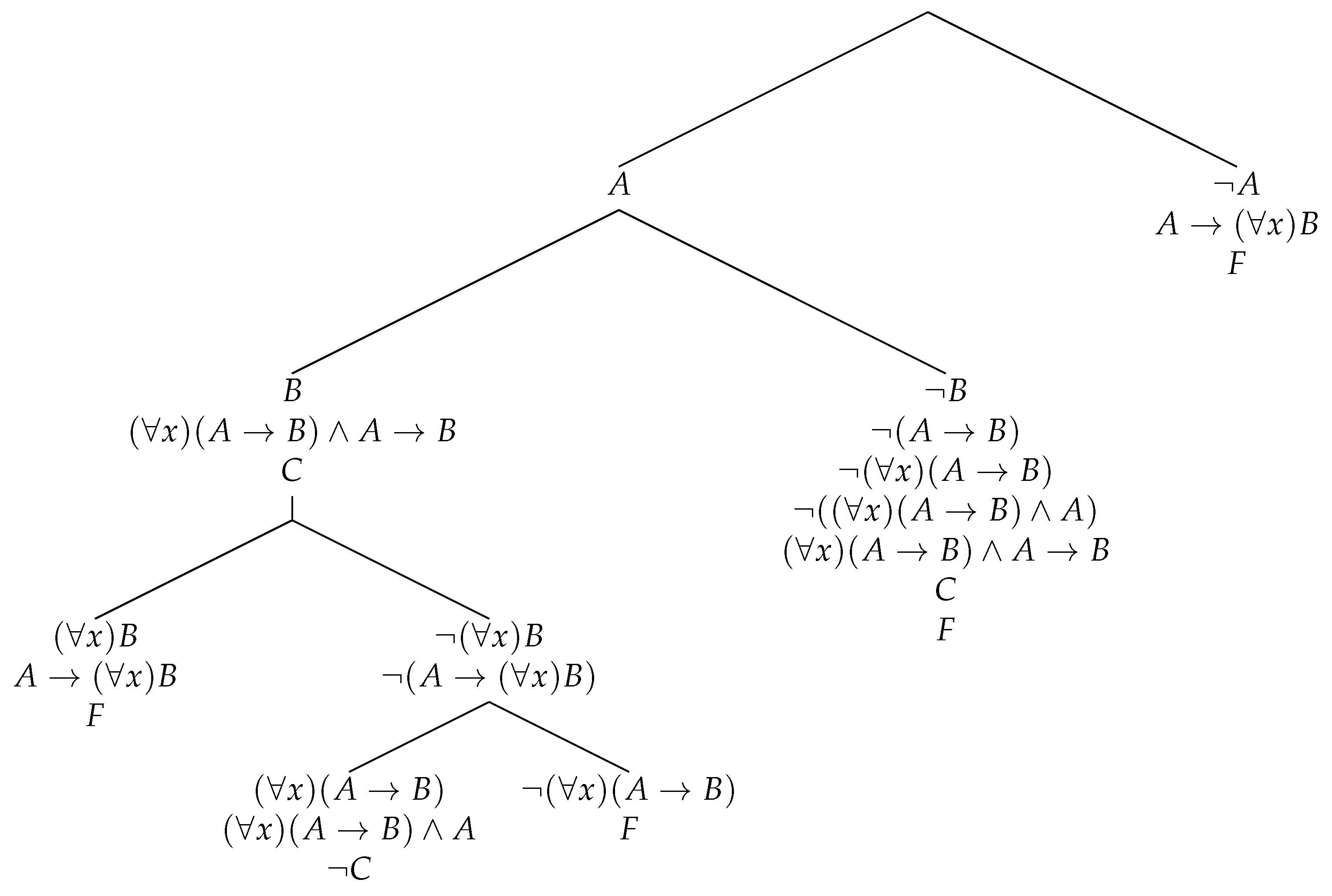
Finally, Figure 4 presents a proof of F where the problematic branch is closed by contradicting formula C. We need to use it, since without “importing” A to the antecedent we cannot generalize on B. Let us also explain that the fourth (from the left) branch contains a kind of a detour: formula ( x ) ( A B ) A B is derived here to make UG 1 applicable in the subtableau starting with A. After deriving formula C, we need to extend the branch with F (obtained by r 1 , which is a local rule), to make the tree a proof of F. The whole tableau is a good example illustrating the fact that the synthetic tableaux system is not a “tableau system” in the common sense of the term.
The interesting reflection is that about the relation between the axiomatic system and that of ST. The latter may seem bizarre, if an axiomatic proof is needed in order to get a hint on how to prove a formula. It appears that heuristics of proving theorems in axiomatic systems may serve also as heuristics of proving theorems in the ST-system. What is the benefit, if any? Does it work also the other way round, that is, is it the case that heuristics suitable for the ST-system can work for axiomatic systems as well?
At the moment, we are not able to answer this questions satisfactorily. However, the example with formula F sheds some light in this darkness. Although we need a hint to prove it, the use of the PB-rule is still restricted to subformulas (as mentioned above, the notion of subformula must take into account all substitutions) of formula F. The more complex formulas are built from the “atoms” introduced by the PB-rule. Albeit this “composition” derives us from the set of subformulas of F, it does so only via the export-import manipulation necessary to generalize on the consequent. This may be a matter of the particular form of rules for universal generalization in this ST-system.

8. ST-Systems for First-Order Theories

In [33], the authors presented a strategy of transforming axioms of certain forms into sequent calculus rules, in order to obtain a sequent calculus for a given first-order theory. In this section, we show that similar techniques may be applied beyond the domain of structural proof theory.

8.1. Universal Axioms

After Negri and von Plato [33], by universal axioms we mean sentences of L FOL of the following form:
( x 1 ) ( x k ) ( A 1 A n B 1 B m )
where A i and B j are atomic formulas. For simplicity, in this section, we assume that both conjunction and disjunction may have an arbitrary number of arguments. We show how the universal axioms can be converted into ST-rules. When n , m 1 , the rule has one of the forms indicated below.
A 1 A 2 A n B 1 B m ( R a x 1 ) A n B 1 | | B m ( R a x 1 ) A 1 A n B 1 B m ( R a x 2 ) A 1 A n B 1 | | B m ( R a x 2 )
Rules ( R a x 1 * ) and ( R a x 2 * ) cause branching to m subtrees. If the local rules for ∨ and ∧ are present in the system, then each of the four rules may be derived from any of the other three. We show two examples of such derivations below, the others are easy to find. On the left: rule ( R a x 1 ) is assumed, rule ( R a x 1 * ) is derived. On the right: rule ( R a x 2 * ) is assumed, rule ( R a x 1 ) is derived. Axioms 08 00133 i014
The general scheme of the proof of (ax) in an ST-system, assuming only atomic cuts and rule ( R a x 1 ) , looks as follows: Axioms 08 00133 i015 If we allow cut-formulas to be non-atomic, we can use the second rule and the proof can be simplified: Axioms 08 00133 i016
Further, for universal axioms (ax) with n = 0 and m 1 , we obtain the following no-premises rules:
B 1 B m ( R a x 1 )
B 1 B m ( R a x 1 * )
At each stage of a derivation, one can introduce the formula (in the case of ( R a x 1 ) ) or extend a tree by means of m subtrees (in the case of ( R a x 1 * ) ). As before, each of this rule is derivable from the other.
If n 1 and m = 0 , the rules can be formulated as follows:
A 1 A n C ( R a x 2 ) A 1 A n C ( R a x 2 )
C is an arbitrary formula. If we had Falsum (⊥) in the language, we could put C = . Again, these rules are inter-derivable in the system. Below to the left, we assume ( R a x 2 * ) and derive ( R a x 2 ) ; and vice versa to the right, where F is for ¬ ( A 1 A n ) : Axioms 08 00133 i017

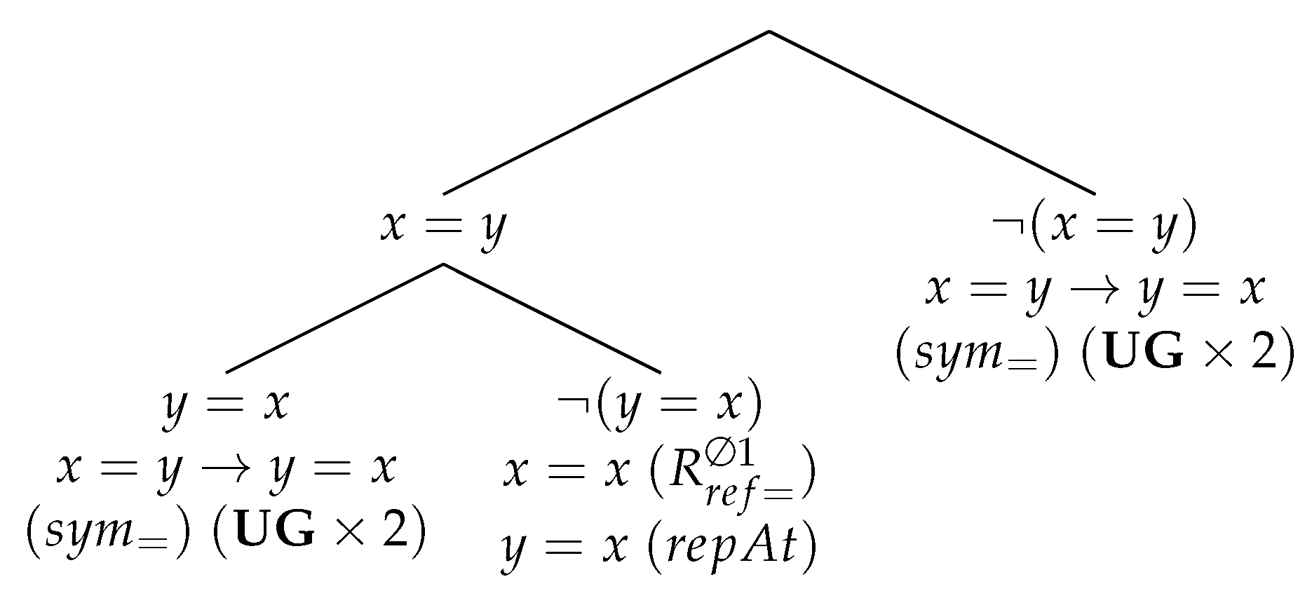
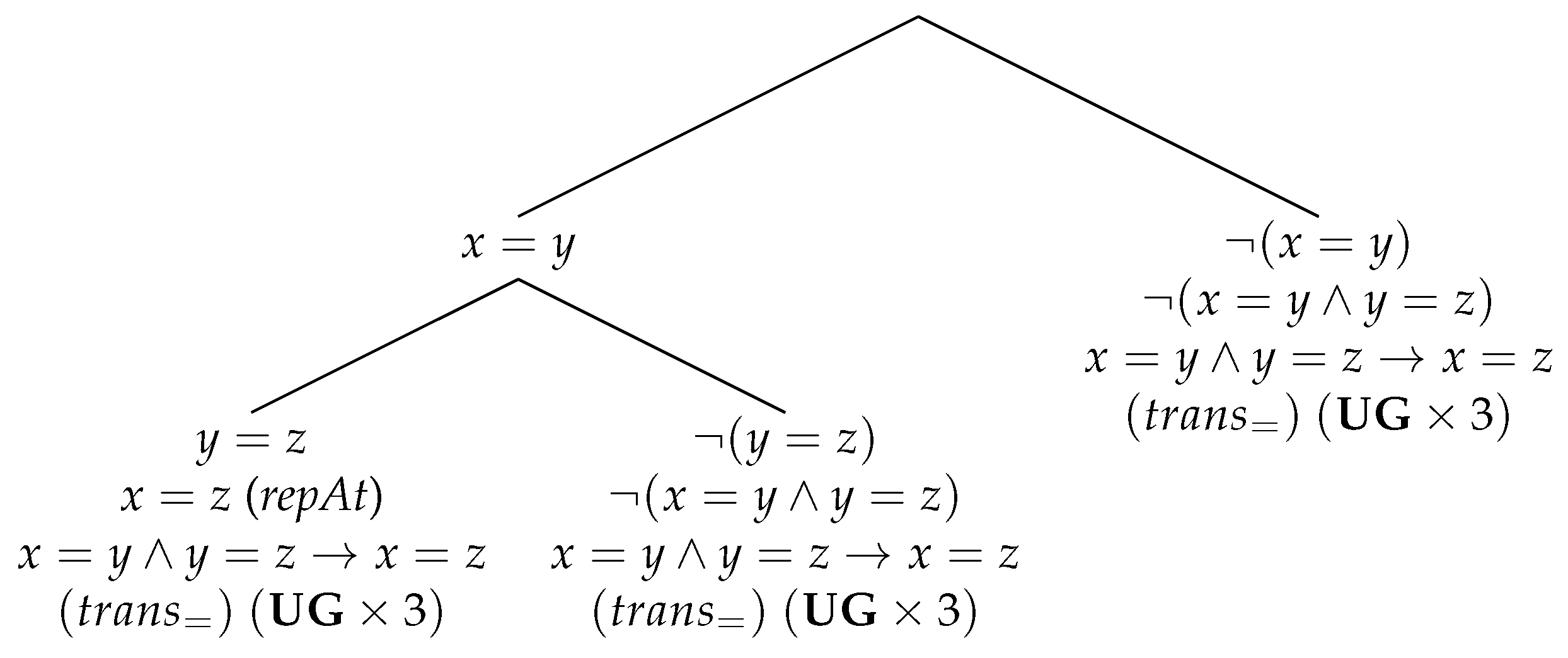
8.2. First Example: Identity

We show how to use the general approach in order to tackle the First-Order Logic with identity. First, we have to extend the language L FOL by means of a special predicate symbol, =, representing identity. Axiomatic system for FOL with identity, F FO = , can be obtained from F FO by the addition of the following two axioms:
( x ) ( x = x )
t i = t j A ( t i ) A ( t j / / t i )
where the notation “ A ( t j / / t i ) ” indicates that some occurrences (possibly all of them) of a term t i in a formula A has been replaced by a term t j . Similarly as in the case of substitutions, if a formula of the form A ( t j / / t i ) is considered, it is assumed that the replacement operation was performed “correctly”, that is, the variables of t i are not bounded in A, and t j is free for each variable of t i in A.
According to the introduced strategy, the axioms correspond to the following two rules:
t = t ( R r e f = 1 ) t i = t j A ( t i ) A ( t j / / t i ) ( R r e f = 1 )
The assumed semantics is model-theoretic, with the identity predicate interpreted as identity in the domain in every interpretation. The rules have a local character, therefore, for the soundness of the whole ST-system, it is enough to check that they have a property expressed in Lemma 1. We skip the details.
ST-system for FOL with identity results from the system designed for FOL in Section 5 by means of extending the latter with the two rules for identity. Let us call the resulting calculus ST FOL = .
Theorem 7
(Completeness). If a formula is provable in F FO = , then it is also provable in ST FOL = .
Proof. 
We know that all the rules of inference of F FO = can be simulated in ST FOL = (Theorem 3). What we have to show is that both axioms are derivable in our system. This is in fact the case as the following derivations show. The first axiom is derivable by: Axioms 08 00133 i018
The derivation starts with branching on x = x . Then, on the right, we use rule ( R r e f = 1 ) , to introduce x = x , which makes the branch closed. Now, the only open branch of the tree is the left one, where the rule UG is applied (let us recall that it is derivable in the ST-system for FOL ).
The second axiom, ( r e p = ) , is derivable by means of the following tree: Axioms 08 00133 i019 This finishes the proof. □
In some systems for FOL with identity, such as natural deduction system (see [33]), it is possible to use a version of the replacement rule restricted solely to atomic formulas. In our setting, such a rule would have the following form:
t i = t j P ( t i ) P ( t j / / t i ) ( r e p A t )
Naturally, the formulas expressing symmetry and transitivity of identity:
( x ) ( y ) ( x = y y = x )
( x ) ( y ) ( x ) ( x = y y = z x = z )
are derivable in ST FOL = , and both are derivable by the use of (repAt). Figure 5 presents a derivation of ( s y m = ) . In Figure 6, ( t r a n s = ) is proved, where on the leftmost branch rule (repAt) is used with x = y for A ( t i ) , y = z for t i = t j , and x = z for A ( t j ) .

8.3. Second Example: Partial Order

The second example of a first-order theory is that of a partial order. We add to the language L FOL a new predicate symbol, ≤, and we build F FO by adding two specific axioms to F FO :
( x ) ( x x )
( x ) ( y ) ( z ) ( x y y z x z )
Following the presented strategy, we transform the first axiom into the following rule:
x x ( R r e f 1 )
which states that at each branch x x can be synthesized without any additional information present.
The second axiom corresponds to the rule:
x y y z x z ( R t r a n s 1 )
We can synthesize x z on the condition that we have already synthesized x y and y z .
If we add these two rules to ST FOL , we obtain a system which we call: ST FOL .
Theorem 8
(Completeness). If a formula is provable in F FO , then it is also provable in ST FOL .
Proof. 
Again, we can derive the rules of inference of F FO as in Theorem 3. We show how the axioms can be derived.
The first axiom is derivable in a manner similar to reflexivity axiom in FOL with identity: Axioms 08 00133 i020 
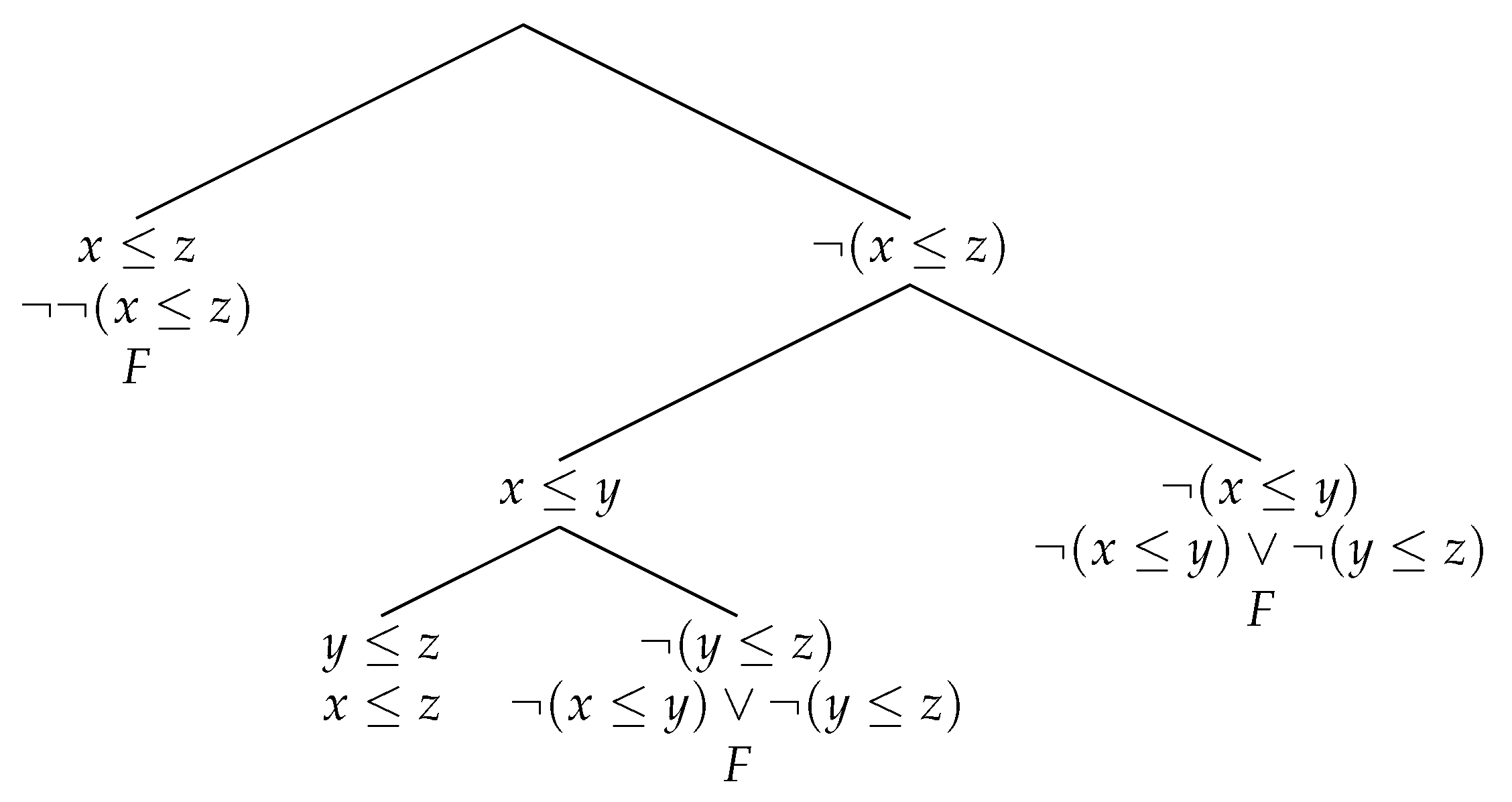
The second axiom is derived as displayed on Figure 7. □
The tree displayed on Figure 8 represents a proof of formula F = ¬ ( x z ) ( ¬ ( x y ) ¬ ( y z ) ) . The formula has been synthesized on every open branch. There is one closed branch containing both x z and its negation.
As in the case of identity, the issue of soundness is settled by verifying that the additional local rules satisfy Lemma 1.
Let us note that the theory of liner order can be obtained from the theory of partial order by means of the addition of the linearity axiom:
x y y x
which corresponds to one of the following rules:
  x y y x ( R l i n 1 )
  x y y x ( R l i n 1 * )
One can easily show that the ST-system for liner order is capable of simulating corresponding axiomatic system, which implies completeness.

9. Conclusions

In this paper, we describe a synthetic tableaux system for First-Order Logic and a general strategy for providing proof systems for some of its axiomatic extensions. We show that the resulting systems are complete with respect to the corresponding axiomatic systems. Synthetic tableaux method was developed to formalize direct validity checking and was inspired by Kalmár’s completeness proof (see [28]). ST system for First-Order Logic is different from the system for propositional logic, due to the fact that one has to introduce global rules, which act on the whole proof tree, while on the propositional level local rules are sufficient.
The rule of cut is, in a sense, essential to this method—it is the rule which starts every derivation introducing the information needed to synthesize more complex formulas. The presence of the cut rule in a system may be an advantage and a disadvantage at the same time. From the proof search oriented perspective, an application of the cut rule is problematic: the rule is unrestricted, so finding the right formula to cut on is hard, even if cut is restricted to subformulas of a goal-formula only. On the other hand, once the right cut formula has been found, the resulting proof may have significantly smaller size than that of proofs constructed by more mechanical methods; we indicate this issue in Section 4.
A step in the same direction has been made before in [34]. The authors proposed a proof procedure for First-Order Logic based on tableaux method with the cut rule. Our work is similar to this proposal in the sense that the cut rule is used while proving theorems and not as the post-processing tool employed to transform already existing derivations to reduce their size. The main difference between the approach in [34] and our approach concerns the proof method used and the form of syntactic structures being processed—in the cited work, the rules act on clauses, whereas our solution does not assume deriving a clausal form.
Finally, we wish to point out some open problems related to the introduced systems. Clearly, there is a connection between Frege systems and ST method, which we think should be further investigated. In particular, a question arises whether proof heuristics working well in one system can be transferred to the other. Another problem pertains to the lack of a subformula property being an effect of unrestricted cut applications. Is there a way to restrict the class of formulas appearing in a proof tree for a given formula?
References

Author Contributions

The first author is mainly responsible for Section 1, Section 2, Section 3, Section 4, Section 5, Section 6 and Section 7, and the second author is mainly responsible for Section 8 and Section 9; however, the general issues as well as many details in the whole paper were discussed and corrected jointly. Conceptualization, D.L.-J. and S.C.; Formal analysis, D.L.-J. and S.C.; Investigation, D.L.-J. and S.C.; Methodology, D.L.-J. and S.C.; Supervision, D.L.-J.; Writing—original draft, D.L.-J. and S.C.; and Writing—review and editing, D.L.-J. and S.C.

Funding

The first version of this paper, prepared by Dorota Leszczyńska-Jasion, was part of the project supported by funds of the National Science Centre, Poland, grant No. 2012/04/A/HS1/00715. The work of Szymon Chlebowski was supported financially by the National Science Centre, Poland, grant No. 2017/26/E/HS1/00127.

Conflicts of Interest

The authors declare no conflict of interest. The funders had no role in the design of the study; in the collection, analyses, or interpretation of data; in the writing of the manuscript, or in the decision to publish the results.

References

  1. Boolos, G. Don’t eliminate cut. J. Philos. Log. 1984, 13, 373–378. [Google Scholar] [CrossRef]
  2. Orevkov, V.P. Lower bounds for increasing complexity of derivations after cut elimination. J. Sov. Math. 1982, 20, 2337–2350. [Google Scholar] [CrossRef]
  3. Statman, R. Lower Bounds on Herbrand’s Theorem. Proc. Am. Math. Soc. 1979, 75, 104–107. [Google Scholar]
  4. Woltzenlogel Paleo, B. Atomic cut introduction by resolution: proof structuring and compression. In Logic for Programming, Artificial Intelligence and Reasoning (LPAR- 16); Lecture Notes in Computer Science; Clark, E., Voronkov, A., Eds.; Springer: Berlin, Germany, 2010; Volume 6355, pp. 463–480. [Google Scholar]
  5. Ebner, G.; Hetzl, S.; Leitsch, A.; Reis, G.; Weller, D. On the Generation of Quantified Lemmas. J. Autom. Reason. 2019, 63, 95–126. [Google Scholar] [CrossRef]
  6. Finger, M.; Gabbay, D. Cut and pay. J. Log. Lang. Inf. 2006, 15, 195–218. [Google Scholar] [CrossRef]
  7. Finger, M.; Gabbay, D. Equal Rights for the Cut: Computable Non-analytic Cuts in Cut-based Proofs. Log. J. IGPL 2007, 15, 553–575. [Google Scholar] [CrossRef]
  8. Urbański, M. Remarks on Synthetic Tableaux for Classical Propositional Calculus. Bull. Sect. Log. 2001, 30, 194–204. [Google Scholar]
  9. Urbański, M. Tabele Syntetyczne a Logika Pytań (Synthetic Tableaux and the Logic of Questions); Wydawnictwo UMCS: Lublin, Poland, 2002. [Google Scholar]
  10. D’Agostino, M. Investigations into the Complexity of Some Propositional Calculi; Technical Monograph; Oxford University Computing Laboratory, Programming Research Group: Oxford, UK, 1990. [Google Scholar]
  11. Mondadori, M. Efficient Inverse Tableaux. J. IGPL 1995, 3, 939–953. [Google Scholar] [CrossRef]
  12. Urbański, M. Synthetic Tableaux for ukasiewicz’s Calculus 3. Log. Anal. 2002, 177–178, 155–173. [Google Scholar]
  13. Urbański, M. How to Synthesize a Paraconsistent Negation. The Case of CLuN. Log. Anal. 2004, 185–188, 319–333. [Google Scholar]
  14. D’Agostino, M.; Mondadori, M. The Taming of the Cut. Classical Refutations with Analytic Cut. J. Log. Comput. 1994, 4, 285–319. [Google Scholar] [CrossRef]
  15. D’Agostino, M. Are Tableaux an Improvement on Truth-Tables? Cut-Free proofs and Bivalence. J. Log. Lang. Comput. 1992, 1, 235–252. [Google Scholar] [CrossRef]
  16. Urbański, M. Synthetic Tableaux and Erotetic Search Scenarios: Extension and Extraction. Log. Anal. 2001, 173–175, 69–91. [Google Scholar]
  17. Smullyan, R.M. Analytic cut. J. Symb. Log. 1968, 33, 560–564. [Google Scholar] [CrossRef]
  18. D’Agostino, M. Tableau Methods for Classical Propositional Logic. In Handbook of Tableau Methods; D’Agostino, M., Gabbay, D.M., Hähnle, R., Posegga, J., Eds.; Kluwer Academic Publishers: Dordrecht, The Netherlands, 1999; pp. 45–123. [Google Scholar]
  19. Indrzejczak, A. Natural Deduction, Hybrid Systems and Modal Logics; Springer: Berlin, Germany, 2010. [Google Scholar]
  20. Urbański, M. Rozumowania Abdukcyjne. Modele i Procedury (Abductive Reasoning. Models and Procedures); Wydawnictwo Naukowe UAM: Poznań, Poland, 2009. [Google Scholar]
  21. Wiśniewski, A. Erotetic Search Scenarios. Synthese 2003, 134, 389–427. [Google Scholar] [CrossRef]
  22. Wiśniewski, A. Questions, Inferences, and Scenarios; Studies in Logic, Logic and Cognitive Systems; College Publications: London, UK, 2013; Volume 46. [Google Scholar]
  23. Leszczyńska-Jasion, D. Erotetic Search Scenarios as Families of Sequences and Erotetic Search Scenarios as Trees: Two Different, Yet Equal Accounts; Technical Report 1(1); Institute of Psychology, Adam Mickiewicz University: Poznań, Poland, 2013. [Google Scholar]
  24. Troelstra, A.S.; Schwichtenberg, H. Basic Proof Theory, 2nd ed.; Cambridge University Press: Cambridge, UK, 2000. [Google Scholar]
  25. Negri, S.; von Plato, J. Structural Proof Theory; Cambridge University Press: Cambridge, UK, 2001. [Google Scholar]
  26. Fitting, M. First-Order Logic and Automated Theorem Proving, 2nd ed.; Springer: Berlin, Germany, 1996. [Google Scholar]
  27. Urbański, M. First-order Synthetic Tableaux; Technical Report; Institute of Psychology, Adam Mickiewicz University: Poznań, Poland, 2005. [Google Scholar]
  28. Kalish, D.; Montague, R. Logic. Techniques of Formal Reasoning, 2nd ed.; Harcourt Brace Jovanovich College Publishers: Fort Worth, TX, USA, 1980. [Google Scholar]
  29. Buss, S.R. Chapter I. “An Introduction to Proof Theory”. In Handbook of Proof Theory; Buss, S.R., Ed.; Elsevier: Amsterdam, The Netherlands, 1998; pp. 1–78. [Google Scholar]
  30. Cook, S.A.; Reckhow, R.A. On the lenght of proofs in the propositional calculus. In Proceedings of the 6th Annual Symposium on the Theory of Computing, Seattle, WA, USA, 30 April–2 May 1974; pp. 135–148. [Google Scholar]
  31. Cook, S.A.; Reckhow, R.A. The Relative Efficiency of Propositional Proof Systems. J. Symb. Log. 1979, 44, 36–50. [Google Scholar] [CrossRef]
  32. Smullyan, R.M. First-Order Logic; Springer: Berlin/Heidelberg, Germany; New York, NY, USA, 1968. [Google Scholar]
  33. Negri, S.; von Plato, J. Proof Analysis: A Contribution to Hilbert’s Last Problem; Cambridge University Press: Cambridge, UK, 2011. [Google Scholar]
  34. Lettmann, M.P.; Peltier, N. A Tableaux Calculus for Reducing Proof Size. In Proceedings of the 9th International Joint Conference on Automated Reasoning, IJCAR 2018, Oxford, UK, 14–17 July 2018; pp. 64–80. [Google Scholar]
Figure 1. A simulation of MP.
Axioms 08 00133 g001
Figure 2. Universal Generalization, part 1.
Axioms 08 00133 g002
Figure 3. Universal Generalization, part 2.
Axioms 08 00133 g003
Figure 4. A proof of F.
Axioms 08 00133 g004
Figure 5. Symmetry.
Figure 5. Symmetry.
Axioms 08 00133 g005
Figure 6. Transitivity.
Axioms 08 00133 g006
Figure 7. A proof of ( t r a n s ) .
Axioms 08 00133 g007
Figure 8. A proof of F = ¬ ( x z ) ( ¬ ( x y ) ¬ ( y z ) ) .
Axioms 08 00133 g008
Table 1. Linear synthesizing rules of the ST-system for CPL .
¬ B B C r 1 C B C r 2 B ¬ C ¬ ( B C ) r 3 B B C r 1 C B C r 2 ¬ B ¬ C ¬ ( B C ) r 3
¬ B ¬ ( B C ) r 1 ¬ C ¬ ( B C ) r 2 B C B C r 3 B ¬ ¬ B r ¬
Table 2. Introduction rules of KI.
f ( B ) t ( B C ) It 1 t ( B ) t ( B C ) It 1 f ( B ) f ( B C ) If 1 t ( B ) f ( ¬ B ) If ¬
t ( C ) t ( B C ) It 2 t ( C ) t ( B C ) It 2 f ( C ) f ( B C ) If 2 f ( B ) t ( ¬ B ) It ¬
t ( B ) f ( C ) f ( B C ) If f ( B ) f ( C ) f ( B C ) If t ( B ) t ( C ) t ( B C ) It
Table 3. Axiom schemes of F .
1. A ( B A ) 6. ( A B ) ( ( A ¬ B ) ¬ A )
2. ( A B ) ( ( A ( B C ) ) ( A C ) ) 7. ¬ ¬ A A
3. A A B 8. A B A
4. B A B 9. A B B
5. ( A C ) ( ( B C ) ( A B C ) ) 10. A ( B A B )

