Article

Wavelet-Based Monitoring for Biosurveillance

Indian School of Business, Gachibowli, Hyderabad 500 032, India
Axioms 2013, 2(3), 345-370; https://doi.org/10.3390/axioms2030345
Submission received: 5 June 2013 / Revised: 18 June 2013 / Accepted: 19 June 2013 / Published: 9 July 2013
(This article belongs to the Special Issue Wavelets and Applications)

Abstract

:
Biosurveillance, focused on the early detection of disease outbreaks, relies on classical statistical control charts for detecting disease outbreaks. However, such methods are not always suitable in this context. Assumptions of normality, independence and stationarity are typically violated in syndromic data. Furthermore, outbreak signatures are typically of unknown patterns and, therefore, call for general detectors. We propose wavelet-based methods, which make less assumptions and are suitable for detecting abnormalities of unknown form. Wavelets have been widely used for data denoising and compression, but little work has been published on using them for monitoring. We discuss monitoring-based issues and illustrate them using data on military clinic visits in the USA.

1. Introduction to Modern Biosurveillance

Biosurveillance is the practice of monitoring data for the early detection of disease outbreaks. Traditional biosurveillance has focused on the collection and monitoring of medical and public health data that verify the existence of disease outbreaks. Examples are laboratory reports and mortality rates. Although such data are the most direct indicators of a disease, they tend to be collected, delivered and analyzed days, weeks and even months after the outbreak. By the time this information reaches decision makers, it is often too late to treat the infected population or to react in other ways. Modern biosurveillance has therefore adopted the notion of “syndromic data” in order to achieve early detection. Syndromic data include information such as over-the-counter and pharmacy medication sales, calls to nurse hotlines, school absence records, web searches for symptomatic keywords and chief complaints by patients visiting hospital emergency departments. These data do not directly measure an infection, but it is assumed that they contain an earlier, though weaker, signature of a disease outbreak. The various data sources fall along a continuum according to their “earliness”. Under the assumption that people tend to self-treat and self-medicate themselves before rushing to the hospital, we expect web searching and purchasing of over-the-counter (OTC) medication to precede calls to nurse hotlines and ambulance dispatches and, then, to be followed by emergency department visits. Still, this entire continuum is assumed to occur before actual diagnoses can be made (after hospitalization and/or lab tests).
Recent years have shown great improvement in the collection and transfer of syndromic data. Currently, many surveillance systems that are deployed across the country routinely collect data from multiple sources on a daily basis, and these data are transferred with very little delay to the biosurveillance systems (see Fienberg and Shmueli [1] and Shmueli and Burkom [2] for a description of this process and examples from several surveillance systems). This means that the multiple syndromic data streams that are now collected are very different in nature from traditional data. We now have multiple time-series that come from different sources and, therefore, have different background behavior. Since these sources are believed to indirectly capture a disease outbreak, they tend to have a lower signal-to-noise ratio than traditional diagnostic data. This means that the noise includes sources of variation that are irrelevant to outbreak detection, such as the correlation of sales of cough medication with overall grocery sales. Almost all series exhibit some type of seasonality, which can differ across sources. The daily frequency of collection leads to non-negligible autocorrelation, and the nature of these non-specific datasets can include missing values (e.g., school absences are missing on holidays), coding errors, etc. Furthermore, the level of stationarity varies across series and across sources. These types of complications were demonstrated for over-the-counter medication sales [1,3]. Figure 1 illustrates some of these features. The top panel describes the daily number of visits to military outpatient clinics in Charleston, North Carolina, that resulted in respiratory complaints. The noisiness and changing mean are visible. During this period, epidemiologists believe that an outbreak occurred between Feb-19 and Mar-20 of 2002. We describe the data, outbreak and further details in Section 3. Zooming in (bottom panel in Figure 1) reveals a clear day-of-week effect, with lower counts on weekends.
A further complication in biosurveillance is that the signature of a disease outbreak in syndromic, and especially non-traditional, data is of an unknown pattern. We do not know how an anthrax attack will manifest itself in ambulance dispatches or in sales of cough remedies. Also, these systems are currently being used for the dual purpose of detecting natural disease outbreaks and bio-terrorist attacks, which can be of a very different nature. Due to this signature uncertainty, it is reasonable that methods that are tuned to particular anomaly patterns (such as classic control charts) will be, on average, less powerful than “general detectors”(Aradhye et al. [4] Note: “existing [control chart] Statistical Process Control (SPC) methods are best for detecting features over a narrow range of scales. Their performance can deteriorate rapidly if the abnormal features lie outside this limited range. Since in most industrial processes the nature of the abnormal features is not known a priori, [wavelet-based] Multiscale Statistical Process Control (MSSPC) provides better average performance, due to its ability to adapt to the scale of the features.”).
Figure 1. Daily number of respiratory chief complaints among visits to military outpatient clinics in Charleston between July 2001 and August 2002 (top) and zoomed-in view during September 2001 (bottom).
Axioms 02 00345 g001
In the absence of syndromic data that contain actual bio-terrorist attacks, there is the additional ambiguity of how to evaluate the performance of different algorithms. Even for natural outbreaks, the assertion of when exactly an outbreak occurred is ambiguous. A pioneering biosurveillance program by the The Defense Advanced Research Projects Agency (DARPA) was aimed at evaluating different algorithms using a common set of syndromic data in multiple US cities. For determining natural outbreaks in the data, a team of epidemiologists and medical specialists were assigned the task of identifying outbreaks. According to Siegrist et al. [5] and as described in Siegrist and Pavlin [6], the team used three methods to determine “golden standards”: documented outbreaks identified by traditional surveillance, visual analysis of the data and simple statistical algorithms to identify anomalies in the data. This, of course, raises issues of how outbreaks and their dates are determined, the circularity of determining outbreaks by employing statistical surveillance and the evaluation of actual detection rates, false alarm rates and timeliness. This adds an additional layer of uncertainty that further distinguishes between biosurveillance and classic engineering process control. An alternative approach has been to seed syndromic data with an artificial outbreak. However, there is a major challenge in constructing realistic outbreak patterns, because the signatures of such outbreaks in syndromic data are yet unknown.
Current surveillance systems rely mostly on traditional statistical monitoring methods, such as statistical process control and regression-based methods, e.g., [7,8]. The simplicity and familiarity of these methods to the public health community have led them to continue being implemented in this new environment. However, it appears that more suitable monitoring methods should evolve, as they have in other fields, where the data environment has changed in this way. This has motivated our investigation of wavelet methods, which have been adopted in many fields and, in particular, are suitable for the type of data and problems in biosurveillance.

2. Wavelet-Based Monitoring

In this section, we focus on how wavelets can be used for the purpose of monitoring and what the important issues that arise are. We start with a brief description of wavelets and the wavelet decomposition, focusing on the parts that are relevant for monitoring. There is a large literature on wavelets and their uses, and this is beyond the scope of this work.
Wavelets are a method for representing a time-series in terms of coefficients that are associated with a particular time and a particular frequency [9]. The wavelet decomposition is widely used in the signal processing world for denoising signals and recovering underlying structures. Unlike other popular types of decompositions, such as the Fourier transform, the wavelet decomposition yields localized components. A Fourier transform decomposes a series into a set of sine and cosine functions, where the different frequencies are computed globally from the entire duration of the signal, thereby maintaining specificity only in frequency. In contrast, the wavelet decomposition offers a localized frequency analysis. It provides information not only on what frequency components are present in a signal, but also when or where they are occurring [10]. The wavelet filter is long in time when capturing low-frequency events and short in time when capturing high-frequency events. This means that it can expose patterns of different magnitude and duration in a series, while maintaining their exact timing.
Wavelet decompositions have proven especially useful in applications where the series of interest is not stationary. This includes long-range-dependent processes, which include many naturally occurring phenomena, such as river flow, atmospheric patterns, telecommunications, astronomy and financial markets ([11], Chap 5). Also, the wavelet decomposition highlights inhomogeneity in the variance of a series. Furthermore, data from most practical processes are inherently multiscale, due to events occurring with different localizations in time, space and frequency [4]. With today’s technology, many industrial processes are measured at very high frequencies, yielding series that are highly correlated and sometimes non-stationary. Together with the advances in mechanized inspection, this allows much closer and cheaper inspection of processes, if the right statistical monitoring tools are applied. The appeal of Shewhart charts has been its simplicity, both in understanding and implementing them, and their power to detect abnormal behavior when the underlying assumptions hold. On the other hand, the growing complexity of the measured processes has lead to the introduction of various methods that can account for features, such as autocorrelated measurements, seasonality and non-normality. The major approach has been to model the series by accounting for these features and monitoring the model residuals using ordinary control charts. One example is fitting Autoregressive Integrated Moving Average (ARIMA) models to account for autocorrelation [12]. A more popular approach is using regression-type models that account for seasonality, e.g., the Serfling model [13] that is widely used by the Centers for Disease Control and Prevention (CDC). A detailed modeling approach is practical when the number of series to be monitored is small and when the model is expected to be stable over time. However, in many cases, there are multiple series, each of differing nature, that might change their behavior over time. In such cases, fitting a customized model to each process and updating the model often is not practical. This is the case of biosurveillance.
An alternative approach is to use a more flexible set of monitoring tools that do not make as many restricting assumptions. Methods that fall into this category are batch-means control charts [14], moving centerline Exponentially Weighted Moving Average (EWMA) [15] and dynamic Principal Components Analysis (PCA) [16]. These methods all attempt to account for autocorrelation in the data. The wavelet decomposition is also such an approach, but it makes even less assumptions: it can handle autocorrelation and non-stationarity.
An additional appeal of wavelet methods is that the nature of the abnormality need not be specified a priori. Unlike popular control charts, such as Shewhart, Cumulative Sum (CuSum), Moving Average (MA) and EWMA charts that operate on a single scale and are most efficient at detecting a certain type of abnormality ([17]), wavelets operate on multiple scales simultaneously. In fact, the Multiscale Statistical Process Control (MSSPC) wavelet-based method ([4]) subsumes the Shewhart, MA, EWMA and CuSum charts. Scales are inversely proportional to frequencies, and thus, cruder scales are associated with higher frequencies.

2.1. The Discrete Wavelet Transform (DWT)

The discrete wavelet transform (DWT) is an orthonormal transform of a real-valued time-series X of length n. Using the notation of Percival and Walden [9], we write w = W X , where w is an n × 1 vector of DWT coefficients and W is an n × n orthonormal matrix defining the DWT. The time-series can be written as:
X t = j = 1 J D j , t + A J , t
where D j = W j w j is the detail associated with changes in X at scale, j, and A J , t is equal to the sample mean. This representation is called the multi-resolution analysis (MRA) of X .
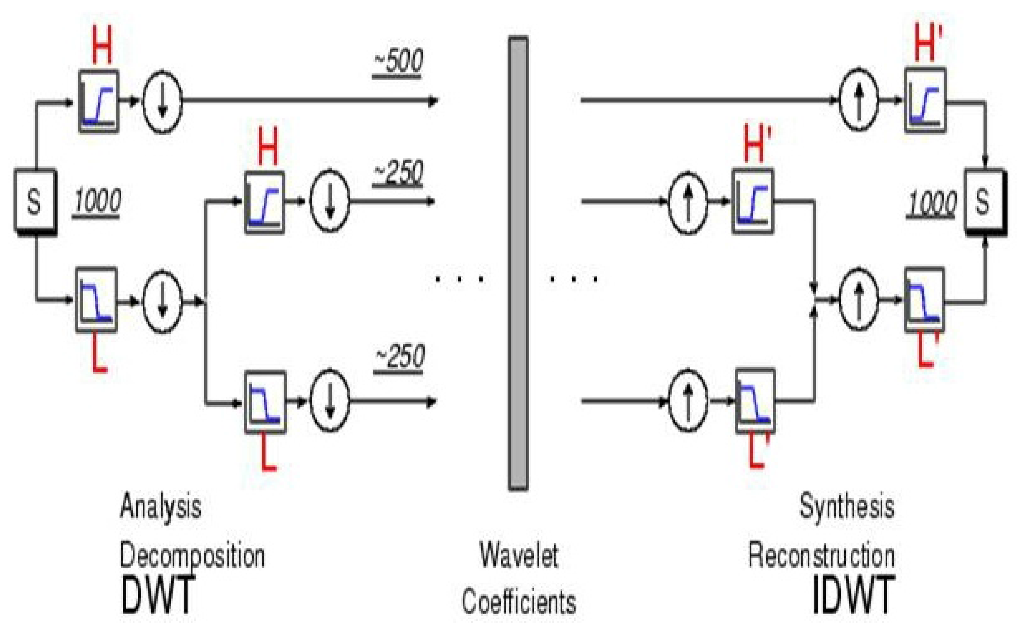
The process of performing DWT to decompose a time-series and the opposite reconstruction step are illustrated in Figure 2. The first scale is obtained by filtering the original time-series through a high-pass (wavelet) filter, which yields the first-scale detail coefficient vector, c D 1 , and through a low-pass (scaling) filter, which gives the first-scale approximation coefficient vector, c A 1 . In the next stage, the same operation is performed on c A 1 to obtain c A 2 and c D 2 , and so on. This process can continue to produce as many as J = log 2 ( n ) scales. In practice, however, a smaller number of scales is used. The standard DWT includes a step of down-sampling after each filtering, such that the filtered output is subsampled by two. This means that the number of coefficients reduces from scale to scale by a factor of two. In fact, the vector of wavelet coefficients, w , can be organized into J + 1 vectors: w = [ c D 1 , c D 2 , , c D J , c A J ] , where c D j and c A j correspond to the detail and approximation coefficients at scale, j, respectively. To reconstruct the series from its coefficients, the opposite operations are performed: starting from c D J and c A J , an upsampling step is performed (where zeros are introduced between each two coefficients) and “reconstruction filters” (or “mirror filters”) are applied in order to obtain c D J - 1 and c A J - 1 . This is repeated, until the original series is finally reconstructed from c D 1 and c A 1 .
Figure 2. The process of discrete wavelet transform (DWT) (from Matlab’s Wavelet Toolbox Tutorial). The time-series (S) is decomposed into three scales.
Axioms 02 00345 g002
Notice that there is a distinction between the wavelet approximation and detail coefficients and the wavelet reconstructed coefficients, which are often called approximations and details. We denote the coefficients by c A and c D (corresponding to approximation and detail coefficients, respectively) and their reconstruction by A and D. This distinction is important, because some methods operate directly on the coefficients, whereas other methods use the reconstructed vectors. The reconstructed approximation, A j , is obtained from c A j by applying the same operation as the series reconstruction, with the exception that it is not combined with c D j . An analogous process transforms c D j to D j .
To illustrate the complete process, consider the Haar, which is the simplest wavelet. In general, the Haar uses two operations: averaging and taking differences. The low-pass filter takes averages ( g = 2 [ 1 / 2 , 1 / 2 ] ), and the high-pass filter takes differences ( h = 2 [ 1 / 2 , - 1 / 2 ] ). This process is illustrated in Figure 3. Starting with a time-series of length, n, we obtain the first level approximation coefficients, c A 1 , by taking averages of every pair of adjacent values in the time-series (and multiplying by a factor of 2 ). The first-level detail coefficients, c D 1 , are proportional to the differences between these pairs of adjacent values. Downsampling means that we drop every other coefficient, and therefore, c A 1 and c D 1 are each of length n / 2 . At the next level, c A 2 coefficients are obtained by averaging adjacent pairs of c A 1 coefficients. This is equivalent to averaging groups of four values in the original time-series. c D 2 coefficients are obtained from c A 1 by taking the difference between adjacent pairs of c A 1 coefficients. This is equivalent to taking the difference between pairwise-averages of the original series. Once again, a downsampling step removes every other coefficient, and therefore, c A 2 and c D 2 are each of length, n / 4 . These operations are repeated to obtain the next scales. In summary, the detail coefficient at scale j, at time t reflects the difference between the averages of 2 j - 1 values before and after time t (the time-series is considered to be at scale j = 0 ).
Figure 3. Decomposition (left) and reconstruction (right) of a signal to/from its coefficients. Decomposition is done by convolving the signal (S) of length n = 1 , 000 with a high-pass filter (H) and low-pass filter (L) and then downsampling. The next scale is similarly obtained by convolving the first level approximation with these filters, etc. Reconstruction is achieved by upsampling and then convolving the upsampled vectors with “mirror filters”. (from Matlab’s Wavelet Toolbox Tutorial).
Axioms 02 00345 g003
The Haar reconstruction filters are given by g * = - g and h * = h . These are used for reconstructing the original series and the approximation and details from the coefficients.
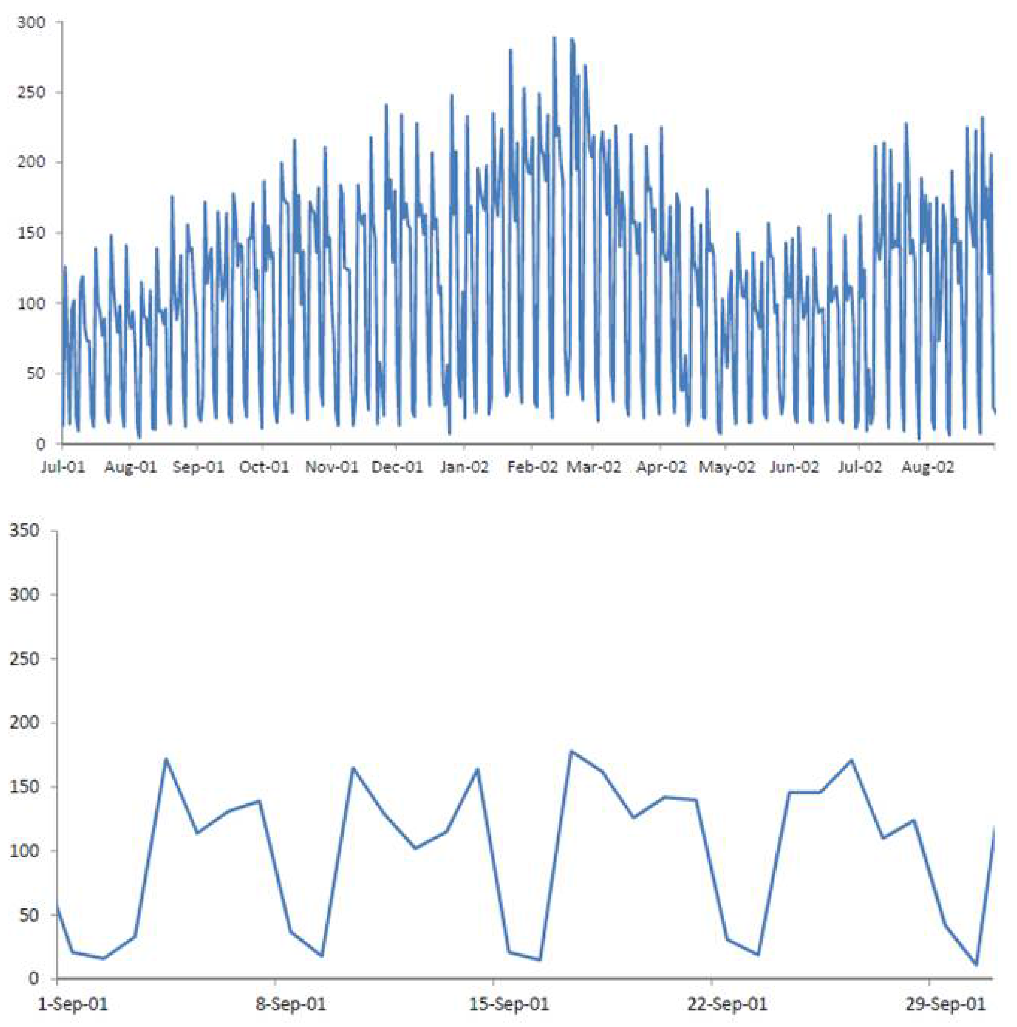
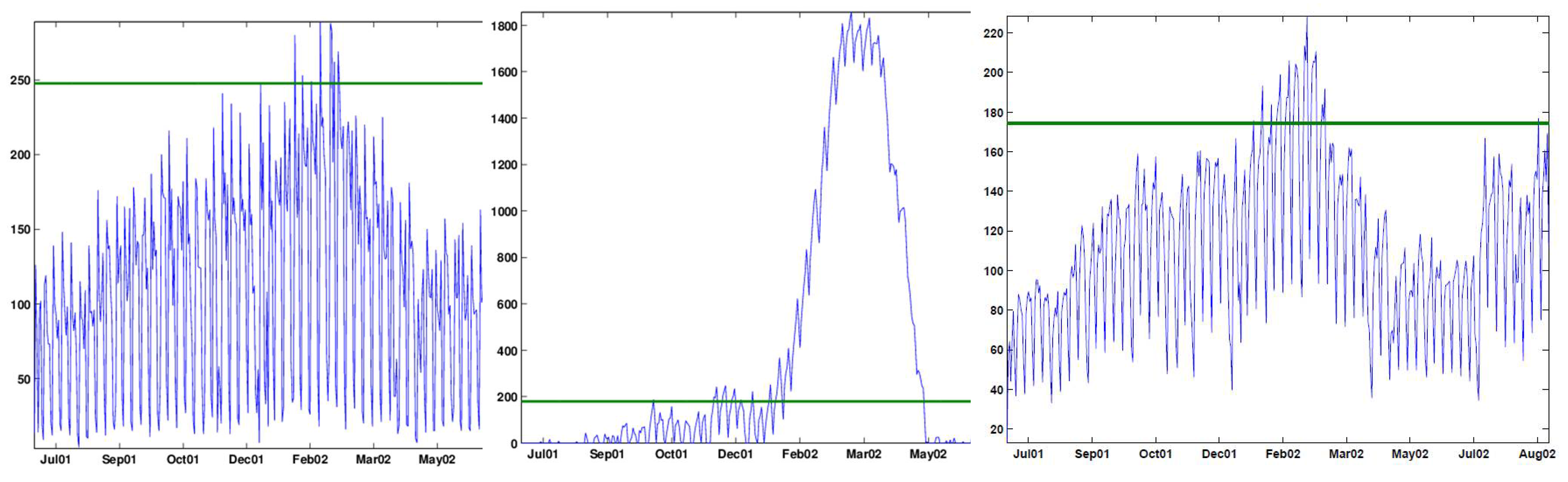
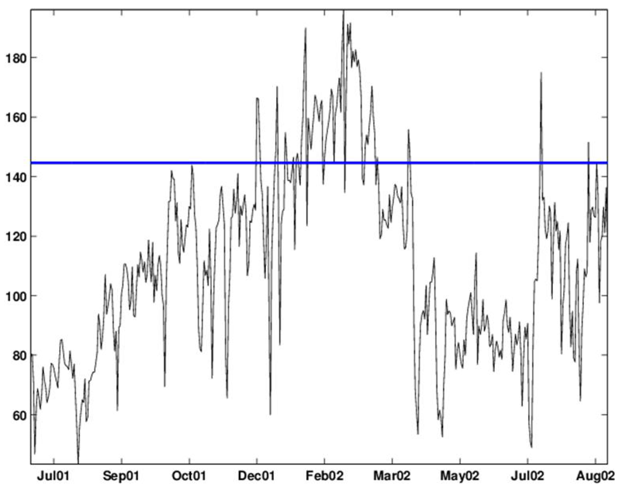
Figure 4 and 
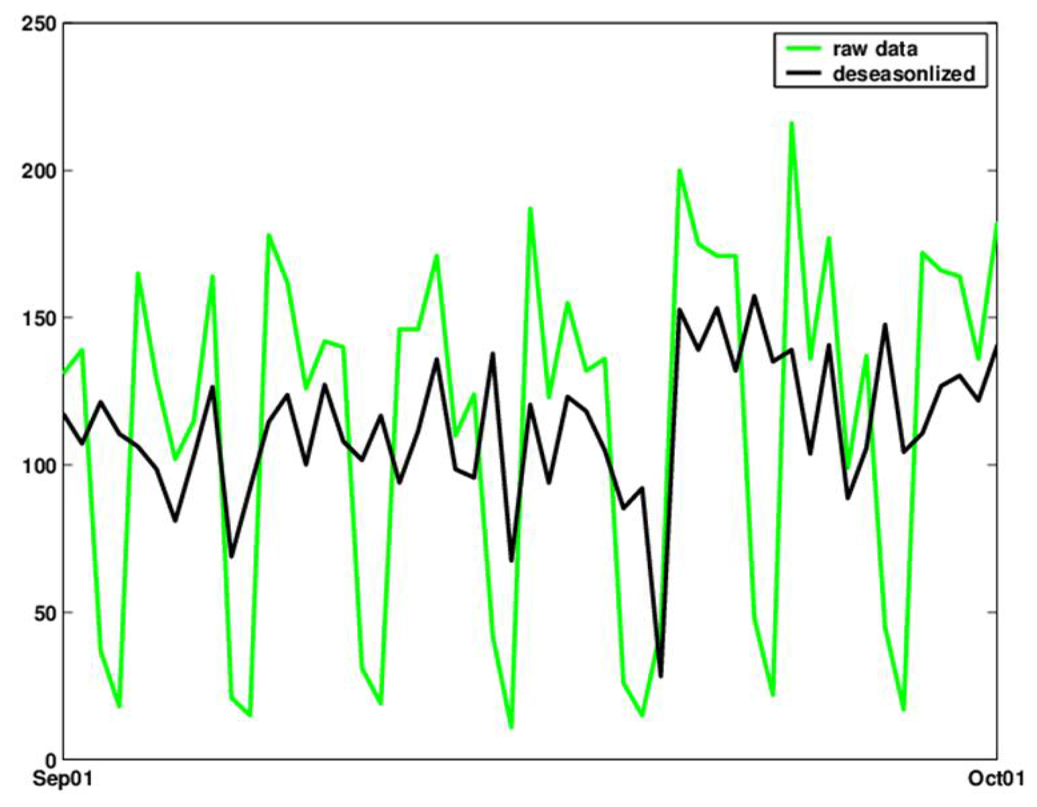
Figure 5 show the result of a DWT with five levels for the (deseasonalized) daily number of visits to military outpatient clinics dataset (deseasonalization is described further in Section 3). Figure 4 displays the Multiresolution Analysis, which includes the reconstructed coefficients ( D 1 - D 5 , A 5 ). Figure 5 shows the set of five detail coefficients ( c D 1 , , c D 5 ) in the bottom panel and the fifth level approximation ( A 5 ) overlayed on top of the original series.
The next step is to utilize the DWT for monitoring. There have been a few different versions of how the DWT is used for the purpose of forecasting or monitoring. In all versions, the underlying idea is to decompose the signal using DWT and then operate on the individual detail and approximation levels. Some methods operate on the coefficients, e.g., [4], while others use the reconstructed approximation and details [18]. There are a few other variations, such as [19], who use the approximation to detrend the data in order to remove extremely low data points, due to missing data. Our goal is to describe a general approach for monitoring using a wavelet decomposition. We therefore distinguish between retrospective and prospective monitoring, where, in the former, past data are examined to find anomalies retrospectively and, in the latter, the monitoring is done in real-time for new incoming data, in an attempt to detect anomalies as soon as possible. Although this distinction has not been pointed out clearly, it turns out that the choice of method, its interpretation and performance are dependent on the goal.
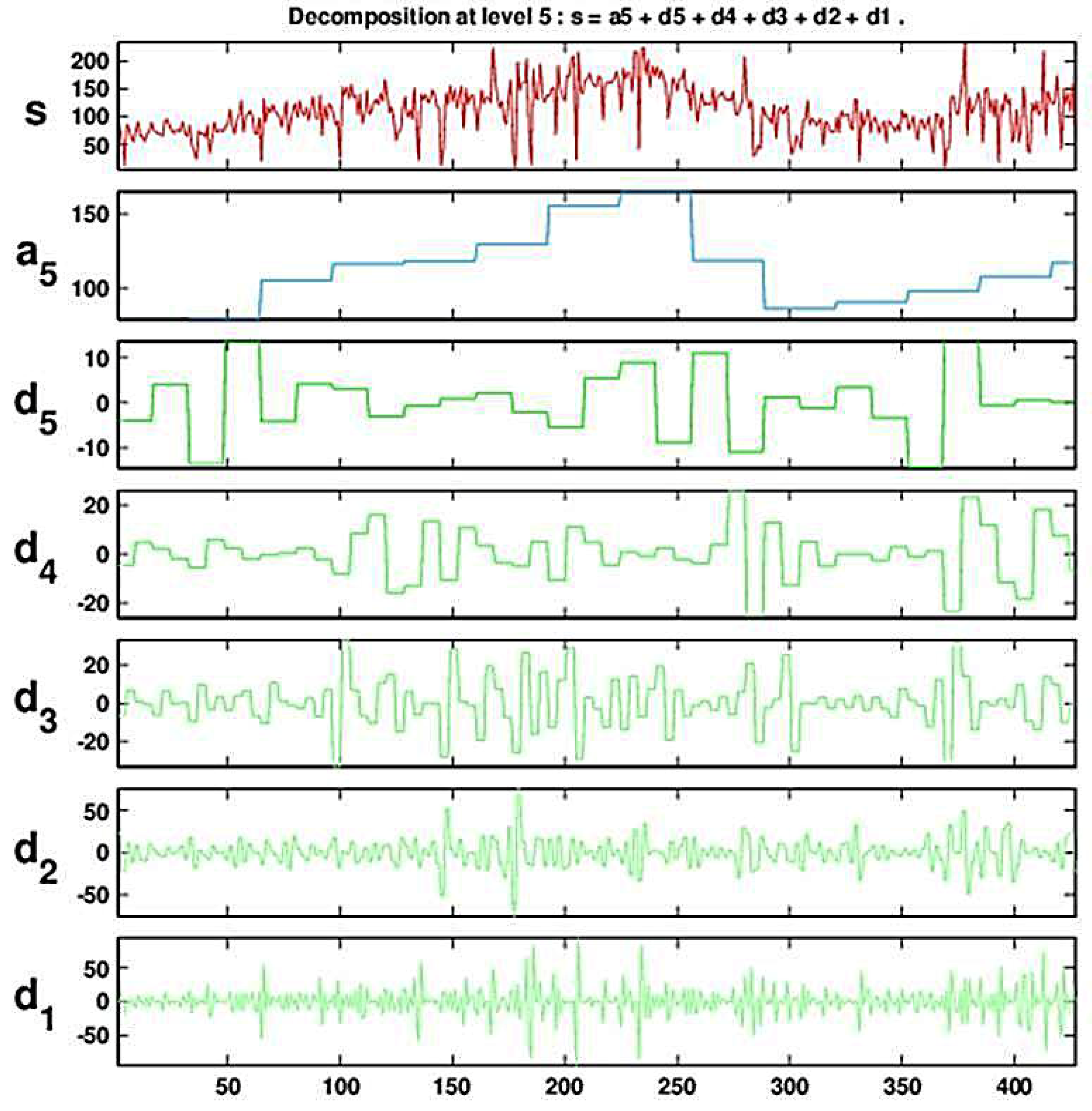
Figure 4. Decomposing the series of daily visits to military outpatient clinics into five levels using the Haar wavelet. The top panel displays the time-series. Below it is the multiresolution analysis that includes the fifth approximation and the five levels of detail.
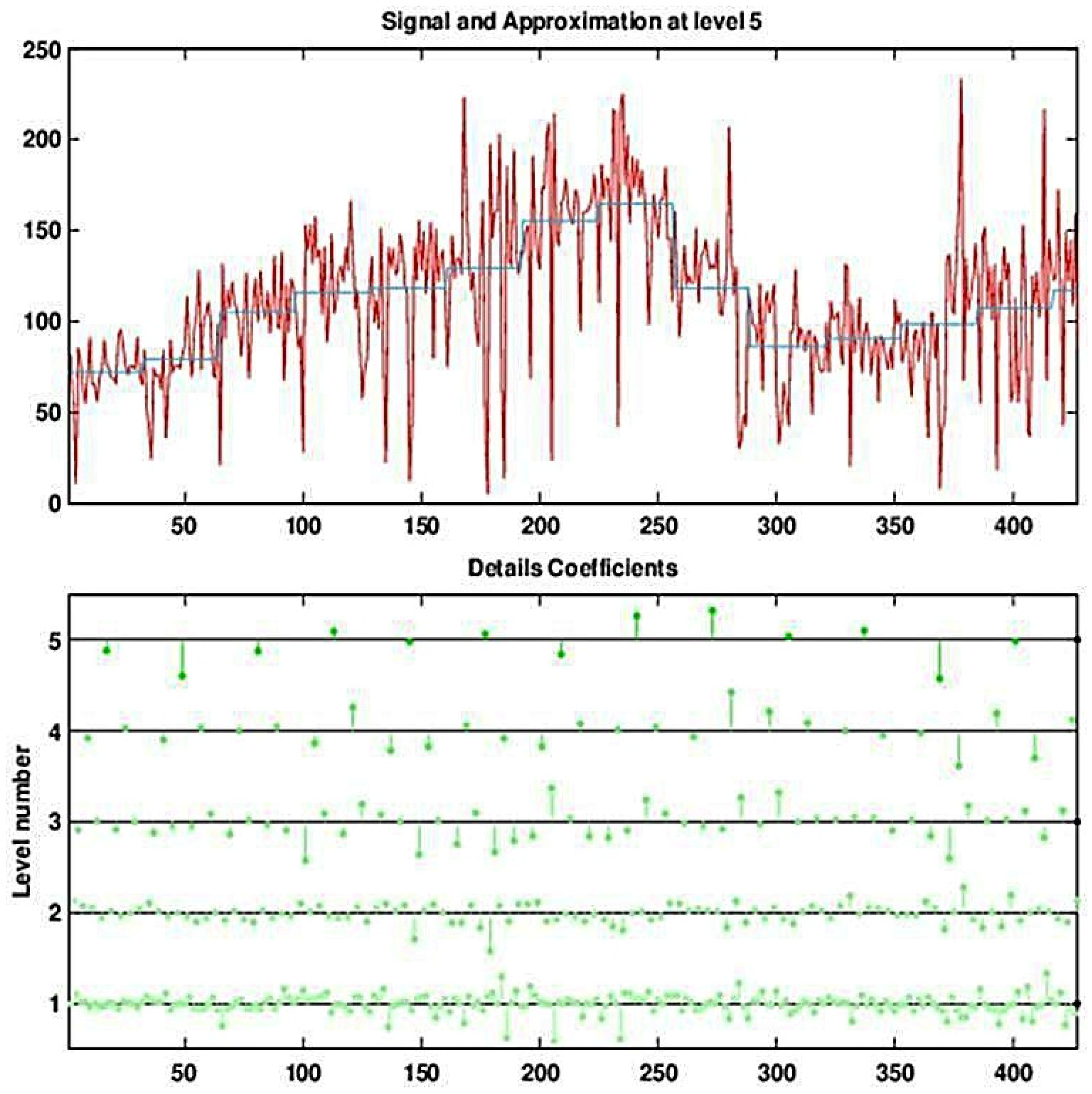
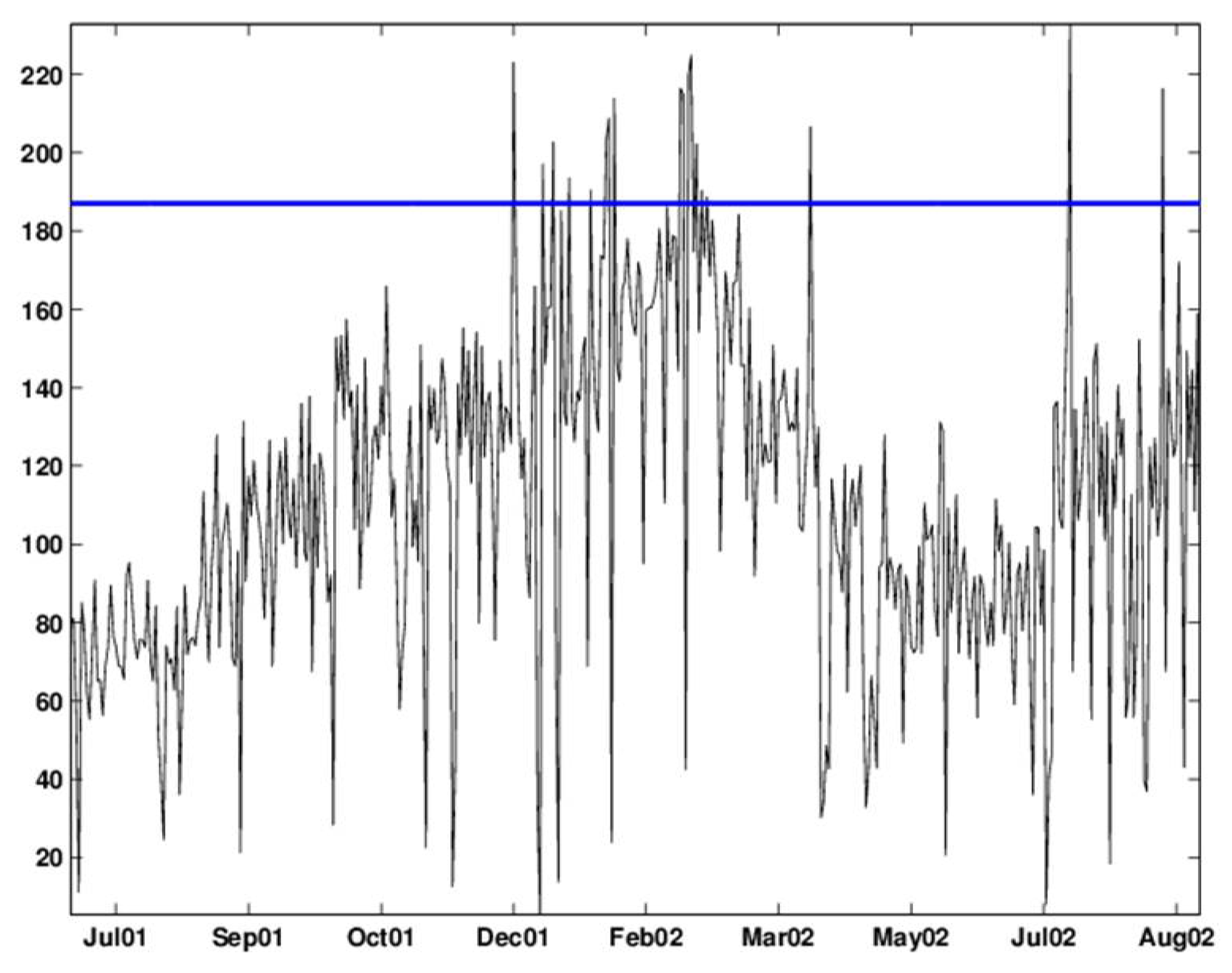
Axioms 02 00345 g004
Figure 5. Decomposing the (deseasonalized) series of daily visits to military outpatient clinics into five levels using the Haar wavelet. The top panel displays the time-series overlaid with the fifth approximation (the blocky curve). The bottom panel shows the five levels of detail coefficients.
Axioms 02 00345 g005

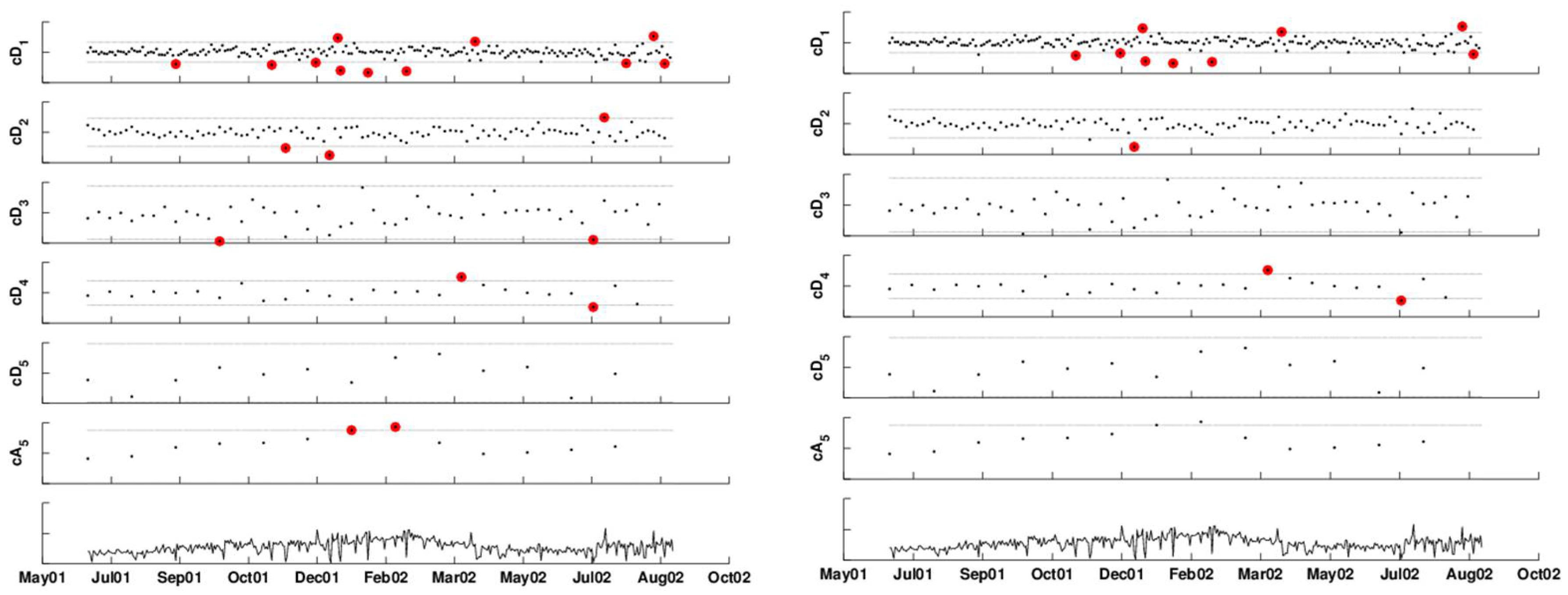
2.2. Retrospective Monitoring

Using wavelets for retrospective monitoring is the easier task of the two. The goal is to find anomalous patterns at any time points within a given time-series. This can be done by constructing thresholds or “control limits” that distinguish between natural variation and anomalous behavior. Wang [20] suggested the use of wavelets for detecting jumps and cusps in a time-series. He shows that if these patterns are sufficiently large, they will manifest themselves as extreme coefficients in the high detail levels. Wang uses Donoho’s universal threshold [21] to determine an extreme coefficient. This threshold is given by σ ( 2 ) log ( n ) / n , where σ is estimated by the median absolute deviation of the coefficients at the finest level, divided by 0.6745 [20].
Another approach that is directly aimed at statistical monitoring was suggested by Bakshi [22]. The method, called Multiscale Statistical Process Control (MSSPC), is comprised of three steps:
  • Decompose the time-series using DWT.
  • For each of the detail scales and for the coarsest approximation scale, construct a Shewhart (or other) control chart with control limits computed from scale-specific coefficients. Use each of the control charts to threshold coefficients so that coefficients within the control limits are zeroed out.
  • Reconstruct the time-series from the thresholded coefficients and monitor this series using a Shewhart (or other) control chart. The control limits at time t are based on estimated variances from scales, where coefficients exceeded their limits at time t.
The method relies on the decorrelation property of DWT, such that coefficients within and across scales are approximately uncorrelated. It is computationally cheap and easy to interpret. Using a set of real data from a chemical engineering process, Aradhye et al. [4] show that this method exhibits better average performance compared to traditional control charts in detecting a range of anomalous behavior when autocorrelation is present or void. Its additional advantage is that it is not tailored for detecting a certain type of anomaly (e.g., single spike, step function, exponential drift) and, therefore, on average, performs better than pattern-specific methods.
MSSPC is appealing, because its approach is along the line of classical SPC. However, there are two points that need careful attention: the establishment of the control limits and the triggering of an alarm. We describe these next.

2.2.1. Two-Phase Monitoring

We put MSSPC into the context of two-phase monitoring: Phase I consists of establishing control limits based on a period with no anomalies. For this purpose, there should be a period in the data that is known to be devoid of anomalies. Phase II uses these control limits to detect abnormalities in the remainder of the data. Therefore, a DWT is performed twice: once for the purpose of estimating standard deviations and computing control limits (using only the in-control period) and once for the entire series, as described in steps 2–3.

2.2.2. Accounting for Multiple Testing

MSSPC triggers an alarm only if the reconstructed series exceeds its control limits. The reconstruction step is essentially a denoised version of the original signal with hard thresholding. An alternative, which does not require the reconstruction step and directly accounts for the multiple tests at the different levels, is described below. When each of the levels is monitored at every time point, a multiple testing issue arises: For an m-level DWT, there are m + 1 tests being performed at every time point in step 2. This results in an inflated false alarm rate. When these tests are independent (as is the case, because of the decorrelation property) and each has a false alarm rate α the combined false alarm rate at any time point will be 1 - ( 1 - α ) m + 1 . We suggest correcting for this multiple testing by integrating the False Discovery Rate (FDR) correction [23,24] into step 2, above. Unlike Bonferroni-type corrections that control for the probability of any false alarm, the FDR correction is used to control the average proportion of false alarms among all detections. It is therefore more powerful in detecting real outbreaks. Adding an FDR correction means, in practice, that instead of setting fixed control limits, the p-values are calculated at each scale, and the thresholding then depends on the collection of p-values.
Finally, using DWT for retrospective monitoring differs from ordinary control charts in that it compares a certain time point not only to its past, but also to its future; depending on the wavelet function, the type and strength of the relationship with neighboring points (e.g., symmetric vs. non-symmetric wavelets and the width of the wavelet filter).

2.3. Prospective Monitoring

The use of DWT for prospective monitoring is more challenging. A few wavelet-based prospective monitoring algorithms were suggested and applied in biosurveillance [e.g., 3,19]. However, there has not been a rigorous discussion of the statistical challenges associated with the different formulation. We therefore list some main issues and suggest possible solutions.
  • Time lag: Although DWT can approximately decorrelate highly correlated series (even long memory with slow decaying autocorrelation function), the downsampling introduces a time lag for calculating coefficients, which becomes more and more acute at the coarse scales. One solution is to use a “redundant” or “stationary” DWT (termed SWT), where the downsampling step is omitted. The price is that we lose the decorrelation ability. The detail and approximation coefficients in the SWT are each a vector of length n, but they are no longer uncorrelated within scales. The good news is that the scale-level correlation is easier to handle than the correlation in the original time-series, and several authors have shown that this dependence can be captured by computationally efficient models. For example, Goldenberg et al. [3] use redundant DWT and scale-specific autoregressive (AR) models to forecast one-step-ahead details and approximation. These forecasts are then combined to create a one-step-ahead forecast of the time-series. Aussem and Murtagh [25] use a similar model, with neural networks to create the one-step-ahead scale-level forecasts. From a computational point of view, the SWT computational complexity is O ( n log 2 n ) , like that of the Fast Fourier Transform (FFT) algorithm, compared to O ( n ) for DWT. Therefore, it is still reasonable.
  • Dependence on starting point: Another challenge is the dependence of the decomposition on what we take as the starting point of the series [9]. This problem does not exist in the SWT, which further suggests the adequacy of the redundant DWT for prospective monitoring.
  • Boundaries: DWT suffers from “boundary problems”. This means that the beginning and end of the series need to be extrapolated somehow in order to compute the coefficients. The amount of required extrapolation depends on the filter length and on the scale. The Haar is the only wavelet that does not impose boundary problems for computing DWT coefficients. Popular extrapolation methods are zero-padding, mirror- and periodic-borders. In the context of prospective monitoring of a time-series, the boundary problem is acute, because it weakens the most recent information that we have. To reduce the impact of this problem, it is better to use wavelets with very short filters (e.g., the Haar, which has a length of two), and to keep the depth of the decomposition to a minimum. Note that an SWT using the Haar does suffer from boundary problems, although minimally ( 2 j values at scale j are affected by the boundary). Renaud et al. [18] and Xiao et al. [26] suggest a “backward implemented” SWT that uses a non-symmetric Haar filter for the purpose of forecasting a series using SWT with the Haar. This implementation only uses past values of the time-series to compute coefficients. Most wavelet functions, excluding the Haar, use future values to compute the coefficients at time n. Examining this modification, we find that it is equivalent to using an ordinary SWT, except that coefficients at scale j are shifted in time by 2 j points. For instance, the level 1 approximation and detail coefficients will be aligned with the second time point, rather than the first time point. This means that at scale j the first 2 j - 1 coefficients are missing, so that we need a phase I that is longer than 2 J . The great advantage of this modification is that new data-points do not affect past coefficients. This means that we can use this very efficiently in a roll-forward algorithm that applies SWT with every incoming point.
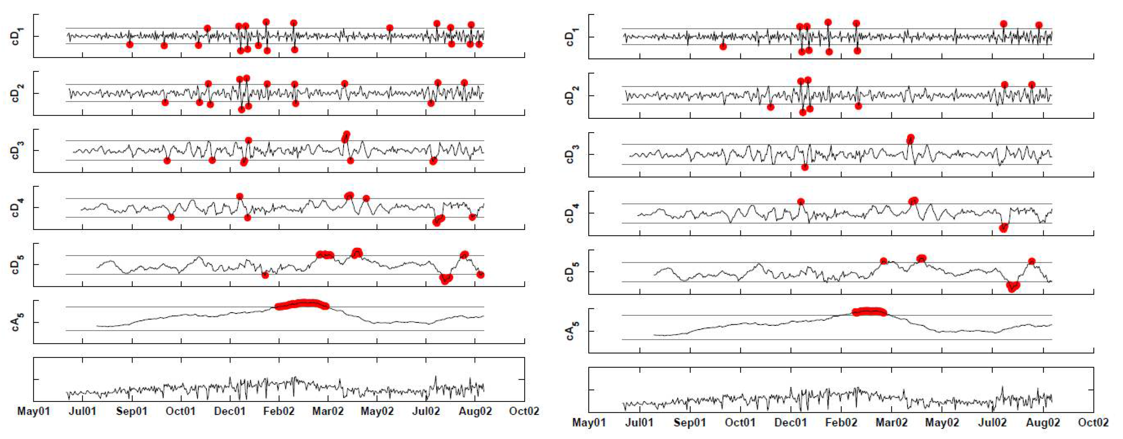
These challenges all suggest that a reasonable solution is to use a Haar-based redundant DWT in its “backward” adaptation as a basis for prospective monitoring. This choice also has the advantage that the approximation and details are much smoother than the downsampled Haar DWT and, therefore, more appealing for monitoring time-series that do not have a block-type structure. Furthermore, the redundant-DWT does not require the time-series to be of special length, as might be required in the ordinary DWT. Finally, the Haar is the simplest wavelet function and is therefore desirable from a computational and parsimonious perspective. 
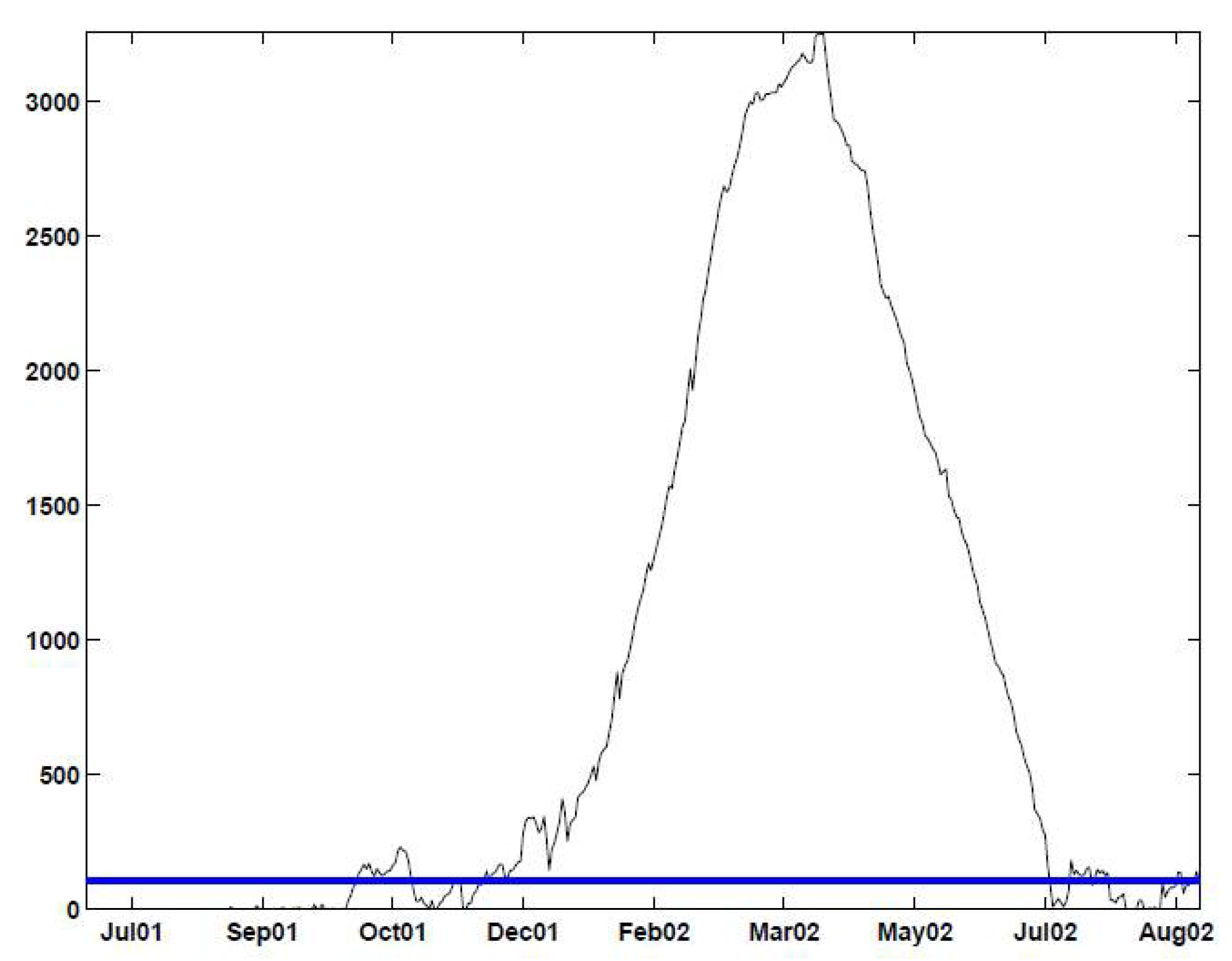
Figure 6 illustrates the result of applying a “backward” redundant Haar wavelet decomposition to the military clinic visits data. It can be seen that the series of coefficients starts at different time-points for the different scales. However, for prospective monitoring, this is not important, because we assume that the original time-series is sufficiently long and that our interest focuses on the right-most part of the series.
Two-stage monitoring should also be implemented in this case: first, a period that is believed to be devoid of any disease outbreak of interest is used for estimating scale-specific parameters. Then, these estimates are used for determining control limits for the alerting of anomalous behavior.
The redundancy in wavelet coefficients now leads to an inflated false alarm rate. Aradhye et al. [4] approached this by determining empirically the adjustment to the control limits in MSSPC when using the redundant DWT. The disadvantage of using the redundant DWT is that the high autocorrelation in the coefficients increases the false alarm rate in highly non-stationary series [4]. An FDR correction can still be used to handle the correlation across scales. In the following, we suggest an approach to handling the autocorrelation within scales directly.

2.3.1. Handling Scale-Level Autocorrelation

As can be seen in Figure 6, the coefficients within each scale are autocorrelated, with the dependence structure being different for the detail coefficients compared with the approximation coefficients series. In addition to autocorrelation, sometimes, after deseasonalizing there remains a correlation at a lag of seven. This type of periodicity is common in many syndromic datasets. The underlying assumption behind the detail coefficients is that in the absence of anomalous behavior, they should be zero. From our experience with syndromic data, we found that the detail coefficient series are well approximated by an autoregressive model of the order of seven with zero-mean.
Figure 6. Decomposing the (deseasonalized) series of daily visits to military outpatient clinics into five levels using the “backward” Haar wavelet, without downsampling. The bottom panel displays the time-series. Above it are the fifth approximation ( c A 5 ) and the five levels of detail ( c D 5 - c D 1 ).
Axioms 02 00345 g006
A similar type of model was also used by Goldenberg et al. [3] to model series arising from a redundant wavelet transform of over-the-counter medication sales. Using an autoregressive model to forecast detail levels has also been suggested in other applications [e.g., 18,
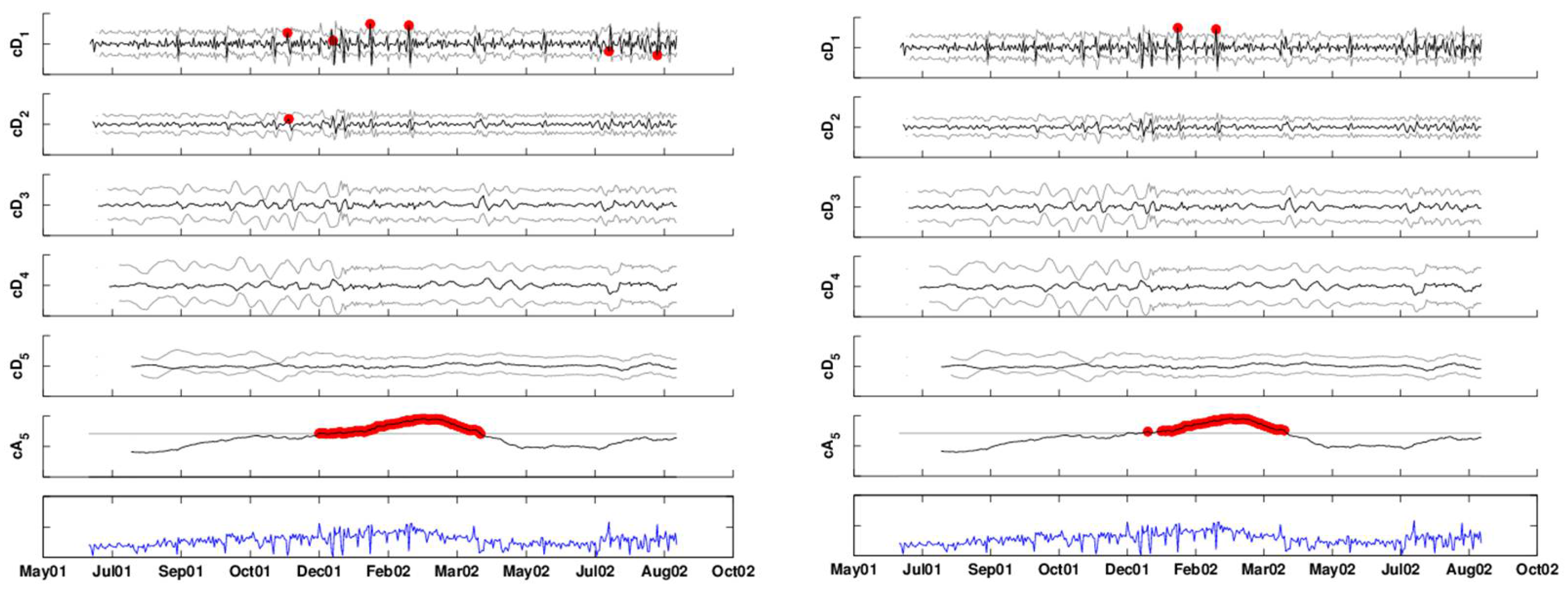
26]. The autoregressive model is used to forecast the coefficient (or its reconstruction) in the next point. In the context of monitoring, we need to specify how the AR parameters are estimated and how to derive forecast error measures. The following describes a roll-forward algorithm for monitoring the coefficients on a new day:
  • Using the phase I period, estimate the scale-specific AR(7) model coefficients ( θ 1 , , θ 7 ) by using the first part of the phase I period and the associated standard deviation of the forecast error ( σ D j ) using the second part of the phase I period.
  • For the phase II data, forecast the next-day detail coefficient at level j ( c D j ( t + 1 ) ), using the estimated AR(7) model:
    c D ^ j ( t + 1 ) = θ ^ 1 c D j ( t ) + θ ^ 2 c D j ( t - 1 ) + + θ ^ 7 c D j ( t - 6 )
  • Using the estimated standard deviation of the forecast error at level j ( σ ^ D j ), create the control limits:
    c D ^ j ( t + 1 ) ± z 1 - α / 2 · σ ^ D j
    where z 1 - α / 2 is the 1 - α / 2 percentile from the standard normal distribution.
  • Plot the next day coefficients on scale-level control charts with these control limits. If they exceed the limits, then an alarm is raised.
The approximation level captures the low-frequency information in the series or the overall trend. This trend can be local, reflecting background noise and seasonality rather than an outbreak. It is therefore crucial to have a sense of what is a “no-outbreak” overall trend. When the outbreak of interest is associated with a bio-terrorist attack, we will most likely have enough “no-outbreak” data to learn about the underlying trend. However, to assess the sampling variability of this trend, we need several no-outbreak seasons. For the case of “ordinary” disease outbreak detection, such as in our example, we have data from a single year, the trend appears to vary during the year, and this one year contains an outbreak period. We therefore do not know whether to attribute the increasing trend to the outbreak or to seasonal increases in outpatient visits during those months. A solution would be to obtain more data for years with no such outbreaks (at least not during the same period) and to use those to establish a no-outbreak trend and its related sampling error. Of course, medical and epidemiological expertise should be sought in all cases in order to establish what is a reasonable level at different periods of the year.
Two methods for evaluating whether there is anomalous behavior using the scale-level forecasts are to add these forecasts to obtain a forecast for the actual new data point (as in [3]). Alternatively, we can compare the actual vs. forecasted coefficient at each scale and determine whether the actual coefficient is abnormal. In both cases, we need estimates of the forecast error variability, which can be obtained from the forecast errors during phase I (the no-outbreak period). For the first approach of computing a forecast of the actual data, the standard deviation of forecast errors can be estimated from the forecasts generated during phase I and used to construct an upper control limit on the original time-series. For the second approach, where scale-level forecasts are monitored directly, we estimate scale-specific standard deviations of the forecast errors from phase I (at scale j, we estimate σ D , j ) and then construct scale-specific upper control limits on the coefficients at that scale. This is illustrated in the next section for our data.
In both cases, the algorithm is implemented in a roll-forward fashion: the scale-level models use the phase I data to forecast the next-day count or coefficients. This is then compared to the actual data or coefficients to determine whether an alarm should be raised. The new point is added to the phase I data, and the forecasting procedure is repeated with the additional data point.
Finally, an important factor for infiltrating new statistical methods into a non-statistician domain is software availability. Many software packages contain classic control charts, and they are also relatively easy to program. For this reason, we make our wavelet-monitoring Matlab code freely available at galitshmueli.com/wavelet-code. The code includes a program for performing retrospective DWT monitoring with Shewhart control limits and a program for performing prospective SWT monitoring with Shewhart or AR-based control limits. In both cases, it yields the control charts and lists the alarming dates. Outputs from this code are shown in the next section.

3. Example: Monitoring Respiratory Complaints at Military Outpatient Clinics in Charleston, SC, between July 2001–August 2002

We return with further detail to the syndromic data that we described in Section 1 and plotted in Figure 1. The data are the daily number of respiratory-complaint visits to military outpatient clinics in Charleston, SC, between July 2001 and August 2002. The respiratory complaints are based on International Classification of Diseases, Ninth Revision (ICD-9) codes. These data were used as part of the Bio-event Advanced Leading Indicator Recognition Technology (Bio-ALIRT) biosurveillance program by The Defense Advanced Research Projects Agency (DARPA) that took place between 2001–2004 (see [6], for further details.)
The underlying assumption is that a disease outbreak will manifest itself earlier in this series than in confirmed diagnosed cases data, by showing an increase in daily visits. However, we do not know the pattern of increase: will it be a single-day spike, an exponential increase or a step function? Furthermore, this time-series exhibits a day-of-week effect, seasonality, dependence and long-term dependence. Finally, a team of epidemiologists detected a gastrointestinal outbreak between February 19 and March 20 of 2002. Such an outbreak is associated with respiratory symptoms. However, as described in Section 1, the determination of this outbreak and its timing must be treated cautiously, as it relies on visual inspection of the data and the use of traditional monitoring tools.
We use this series to illustrate the performance of ordinary control charts (that are the standard tool in biosurveillance) and compare it to wavelet-based monitoring.
Common practice in biosurveillance is to use a standard control chart, such as a CuSum, or an EWMA chart to monitor the raw data (or its standardized version). For instance, Ivanov et al. [27] use EWMA to monitor daily hospital visits by children under the age of five, who have respiratory and gastrointestinal complaints. Common false alarm rates that have been acceptable in biosurveillance are much higher than in engineering practices. The different algorithms in the Bio-ALIRT project report rates of a false alarm every 2–6 weeks. If for our 427-day data, we aim for this rate, we expect approximately 10–30 days with false alarms. However, we hypothesize that the actual false alarm rate from control charts, such as Shewhart, CuSum and EWMA, will be higher than the one we set it to, because of the positive autocorrelation. We therefore set all alarm rates in the following to one in 100 days (≈4 days in our time-series).
Figure 7 illustrates the outcome of applying a one-sided Shewhart x-chart (with a 2.33-sigma upper limit), a one-sided CuSum (with k = 0 . 5 , h = 2 . 84 , using Sigmund’s formula) and a one-sided EWMA chart (with λ = 0 . 4 and a 2.33-sigma upper limit) directly to the raw data. The first 284 days (July 1 to December 31, 2001) served as the phase I period and were used to compute the control limits.
The Shewhart chart alarms on nine days: December 26, 2001, January 22 and 28, 2002, and February 4, 11, 19, 20, 22 and 25, 2002. All of these are weekdays, with the majority being Mondays. The CuSum alarms around five periods: a single alarm on Friday October 12, 2001, a month-long period with most days between November 28 to December 28, 2001, a five-month period between January 10, 2002, and May 10, 2002, a single alarm on Friday July 12, 2002, and a week starting in August 23, 2002 (Friday to Friday). The EWMA alarms on every Friday between January 11, 2002, and March 8, 2002, with a few other weekdays in between. It alarms again on Friday, August 23, 2002. The common features to all charts are the lack of alarms on weekends and alarms around January–February. The last two charts also both alarm in late August, 2002.
Figure 7. Shewhart x-chart (left), Cumulative Sum (CuSum) (center) and Exponentially Weighted Moving Average (EWMA) chart (right) applied to raw data.
Axioms 02 00345 g007
This brings up the important issue that syndromic data typically contain some periodicity. In our data, there is an obvious seven-day periodicity. A close look shows that weekends (Saturday–Sunday) experience, on average, much fewer visits than weekdays, as expected. In addition, Mondays seem to incur the most visits. Applying a Shewhart, CuSum or EWMA chart directly to periodic data, and especially using the periodic data to compute control limits, will obviously deteriorate their performance in two directions: the false alarm rate on days with high counts will increase, and the power of true detection on days with low counts will decrease. For our data, we therefore expect more false alarms on Mondays and low detection power on weekends. The control chart alarm days above indeed support this bias. Seasonality, therefore, should be accounted for before applying these control charts.
Forsberg et al. [28] apply a preliminary step of smoothing using a moving average with a window of seven days to remove daily variation. However, this type of preliminary temporal averaging means that timeliness is sacrificed. Siegrist et al. [5] describe a similar step and reported that “pre-filters using 2–7 day averages were also tried, and the detection delay defeated any gain from the data smoothing.” Other methods for accounting for day-of-week effects have been to model various days of the week as separate time-series and taking differences at a lag of seven.
A simple alternative that does not introduce temporal delays is to deseasonalize the series using the ratio-to-moving averages method [see, e.g., 29, Chapter 13]. The deseasonalized series can then be monitored using a standard control chart. Figure 8 shows the original and deseasonalized data (where day-of-week is removed) for September 2001, using the ratio-to-moving-averages method with multiplicative seasonal indexes.
Figure 8. Raw counts (green) and deseasonalized (bold black) counts of daily visits during the month of September 2001.
Axioms 02 00345 g008

3.1. Using Standard Control Charts

Figure 9, Figure 10 and Figure 11 display three standard (one-sided) control charts applied to the deseasonalized data: a 2.33-sigma Shewhart chart (9), a CuSum chart with k = 0 . 5 , h = 2 . 84 (10) and an EWMA chart with λ = 0 . 4 (11). As before, the first 284 days (July to December of 2001) were used to compute the control limits (phase I), and the alarm rate (under the i i d assumption) was chosen for all cases to be 0.01.
Figure 9. Shewhart chart with an upper 2.33-sigma limit applied to the deseasonalized data. The chart signals alarms on: December, 15, 26 and 30, 2001, January 5, 13, 19–22, 2002, February 16, 17, 19, 20, 22, 24 and 26, 2002, April 6, 2002, July 13, 2002, and August 17, 2002.
Axioms 02 00345 g009
Figure 10. CuSum chart with k = 0 . 5 and h = 2 . 84 applied to the deseasonalized data. The chart signals alarms around five periods: October 13, 2001 to November 2, 2001; November 19–20, 2001, November 30, 2001 to July 4, 2002; July 13–27,2002, and August 23–31, 2002.
Axioms 02 00345 g010
Figure 11. EWMA chart with λ = 0 . 4 and an upper 2.33-sigma limit applied to the deseasonalized data. The chart signals alarms on: December 15–17 and 29–30, 2001, and January 5–6, 11 and 13–14, 2002; most days between January 17, 2002 and March 14, 2002; and April, 6–7, 2002 and July 13, 2002, and 17-Aug-2002.
Axioms 02 00345 g011
Even with the reservation regarding the actual outbreaks in the data, it appears that the control charts are yielding too many false alarms relative to the 1% rate (≈4 days) that they were set to. In all charts, alarms are triggered around December–January, but the spread in dates is very large and not practical for deriving conclusions about outbreak dates. The CuSum and EWMA also alarm from mid-July, 2002 on. However, because of the reliance of these control charts on the assumptions that are violated here, interpreting their signals is questionable. Finally, these charts are used in the same way for retrospective and prospective monitoring, because the daily statistic never relies on future values of the series.

3.2. Wavelet-Based Monitoring

We now use the DWT and SWT to decompose the deseasonalized data. We first decompose the first 284 days (July to December of 2001) in order to compute the control limits (phase I), as in the ordinary control chart case. In both cases, we use the Haar wavelet and five levels of decomposition, because it is reasonable to compare a daily count with neighboring days up to a month (level 5 looks at a window of 32 days).

3.2.1. Retrospective Monitoring

The left panel in Figure 12 shows the DWT of the (seven-day deseasonalized) series, with a two-sided 2.58-sigma x-bar chart applied to each of the detail levels and a one-sided upper 2.33-sigma chart applied to the approximation level (because we are only interested in increases in the series). Different seasonal components can be seen at the different detail levels and possibly in the approximation. If at least one coefficient exceeds its thresholds on a certain day, it signals an alarm. Detail coefficients that are below the lower threshold indicate that the current period has lower counts than the next period, and the opposite holds for detail coefficients exceeding the upper threshold.
In this example, almost all alarms are triggered by the finest detail coefficients, indicating that the number of respiratory complaint visits on certain days (especially in January–March, 2002) was high relative to their neighboring day (after accounting for the day-of-week effect). There is also alarming based on comparison with the counts two weeks previously. Note that alarms are triggered also by the approximation level. However, it is unclear whether this indicates an abnormal increase in the series or else it reflects “natural” seasonality in clinic visits during that period of the year. We discuss this ambiguity further in the next section. The right panel applies an FDR correction to the above results, to account for the multiple testing that occurs on many days. This results in reducing the alarm dates to 12 days: first, on November 12, 2001, where the negative level-1 detail coefficient indicates that this Monday is much lower than the following Tuesday. The second period is December 14, 24, and 30, 2001 and January 1, 2002. Then, during the assumed 2002 outbreak period: January 21, February 18. And finally, a set of single-day alarms in 2002: March 30, April 9, July 4, August 17 and August 25.

3.2.2. Prospective Monitoring

As discussed earlier, DWT is better suited for retrospective surveillance than for prospective surveillance. Instead, we use SWT, which is an undecimated (non-downsampled) DWT, implemented in a “backward” fashion, so that coefficients at time t are computed only using data before time t. This is mathematically equivalent to a roll-forward algorithm that starts after Phase I ends and performs this SWT version every day until Aug 31, 2002.
Figure 13 shows the result of decomposing the data by SWT and applying a 3-sigma x-bar chart to each scale. It can be seen that, as expected, the coefficients within each scale are no longer approximately decorrelated, as are coefficients across scales. The FDR correction is used to correct for the correlation across scales, and the right panel shows the remaining alarms after applying the FDR correction.
Figure 12. DWT of the time-series with 3-sigma x-bar charts applied at each scale. The left panel shows alarms based on coefficients that exceed the thresholds. The right panel shows alarms after correcting for multiple testing.
Axioms 02 00345 g012
Figure 13. Backward-implemented stationary discrete wavelet transform (SWT) with 3-sigma x-bar charts applied at each scale. The left panel shows alarms based on coefficients that exceed the thresholds. The right panel shows alarms after correcting for multiple testing.
Axioms 02 00345 g013
Even after the FDR correction, we get alarms for long periods of time: the first is between January 17 and February 25, 2002 and then, we get three single day alarms on June 22, June 30, and August 13, 2002. These results are not trustworthy, because of the heavy correlation within each scale. We therefore used AR(7) models to forecast the next-day detail coefficients. Using the phase I period, we estimated the scale-specific model coefficients using the first 92 days and the associated standard deviation of the forecast errors from the next 92 days. The estimates are given in Table 1.
Monitoring the approximation level is challenging in our example, because we have data only on a single year, and it supposedly contains an outbreak of the type we are interested in detecting. It is therefore unknown whether the increasing trend during the January–March, 2002, period is due to the outbreak or to other unrelated reasons. In this case, it is necessary to have more data on the January–March season, where it can be asserted that no outbreak of this type has occurred. For the sake of illustration, let us assume that past data indicate that there is no increasing trend during January–March in such syndromic data. In that case, we can use a chart, such as an EWMA, to monitor the approximation coefficient series (because of the autocorrelation). The right panel of Figure 14 shows the result of applying an FDR correction for the multiple testing. Therefore, here, we are accounting for both correlation within scales and across scales. The remaining alarms occur twice in the finest detail coefficients (January 21, 2002, February 18, 2002), and the remaining are all in the approximation (December 12, 2001, and January 9, 2002 to April 9, 2002.) Recall that this is based on an assumption that the trend increase during these months does not reflect the normal behavior of this series. In the presence of data on more years, we would have been able to assess this better and fit a model to the approximation series based on the trend information.
Table 1. Estimated coefficients and standard deviation of forecast errors for scale-level AR(7) models, based on the first 184 days.
c D 1 c D 2 c D 3 c D 4 c D 5
θ ^ 1 −0.87460.73670.85801.00400.9760
θ ^ 2 −0.6520−1.13210.0177−0.09900.2617
θ ^ 3 −0.47580.8163−0.10590.0637−0.0174
θ ^ 4 −0.3598−0.8944−0.6849−0.1315−0.1596
θ ^ 5 −0.32050.49810.60030.0631−0.1195
θ ^ 6 −0.2248−0.3905−0.07050.0285−0.1017
θ ^ 7 −0.16100.1352−0.0986−0.14130.1209
σ ^ e j 23.115.210.67.44.0
Figure 14. Monitoring each scale separately to account for autocorrelation: the detail coefficients (top five panels) are compared to control limits based on an AR(7) model. The approximation coefficients (sixth panel) are monitored by an EWMA chart. The bottom panel is the deseasonalized series. The left panel displays alarms based on exceeding thresholds. The right panel displays alarms after False Discovery Rate (FDR) correction.
Axioms 02 00345 g014
Residual plots indicate that the model residuals are approximately normally distributed, and thus, we can use Equation (3) to construct control limits for the coefficient series. This is shown in the top five panels of Figure 14.
Finally, we can see that the prospective monitoring gives different (and, in this case, fewer) alarms compared to the retrospective monitoring. This is because the prospective algorithm assesses coefficients by comparing them only to their past, whereas the retrospective algorithm compares each point to its past and future.

4. Conclusions and Future Directions

The goal of this paper is to introduce the important area of modern biosurveillance and the challenges that it poses to traditional statistical monitoring. There are currently not many statisticians involved, and there is a pressing need to develop improved biosurveillance systems. From a research point of view, there are opportunities for developing statistical methodology for improving the development and evaluation of biosurveillance systems.
Three components make biosurveillance challenging. First, like many other fields, the advancement of technology has lead to data that are more complex than those collected a century ago. More frequent and diverse data mean that the classical assumptions of sample-to-sample independence and stationarity tend not to be met. This challenge is not specific to biosurveillance and is apparent in chemical processes and geo-physical data, among others. Second, modern biosurveillance systems monitor diagnostic and non-traditional pre-diagnostic data that are assumed to contain an earlier signature of an outbreak than actual diagnosis data. However, this earliness comes at the cost of a weaker outbreak signal compared to actual diagnosis data. Therefore, detecting the weak signal requires sensitive and timely monitoring methods.
Third, since there are nearly no diagnostic data containing bio-terrorist outbreaks, it is unknown how such an outbreak would manifest itself in the data. This means that classic control charts that are specialized in detecting a particular type of pattern (e.g., a single spike, an exponential increase or a linear trend), are risky. Methods that are “general detectors” reduce the risk by “diversifying” the detection to a wider number of patterns. This situation also occurs in other fields, where the outbreak nature might not be known a priori (e.g., in forecasting storms). Future work should therefore investigate the ability of wavelet-based methods to detect different outbreak signatures. Lotze et al. [30] and Cheng et al. [31] propose methods for simulating and evaluating biosurveillance data and outbreaks, which, in turn, can be used for testing the performance of wavelet and other methods.
Finally, the issue of the lack of “golden standards” is a major challenge. The problem is that determining whether an outbreak of interest is contained in the data is not straightforward. The current practice is for a team of medical staff and epidemiologists to eyeball a few series of syndromic data in order to determine whether and when an outbreak started. This clearly results in tuning and developing monitoring tools for detecting what the team sees, rather than actual outbreaks in the data. Furthermore, it greatly complicates the evaluation of algorithms and their performance. The implications of not having golden standards are: (1) When the goal is to detect natural outbreaks, and we do not know whether and when exactly in the data there are such outbreaks, it is hard to assess what is a phase I in order to estimate process in-control parameters and to establish control limits; (2) when the goal is to detect outbreaks associated with bio-terrorist attacks, we can (luckily) assume that the data are clean of such attacks. However, the presence of natural outbreaks in the data create more background noise that is hard to model if it is not specified as an outbreak. One approach has been to try and seed the data with outbreaks (e.g., Goldenberg et al. [3], Stoto et al. [32]). This avoids the lack of data with a certain outbreak signature in it, but we still have the problem of determining whether other outbreaks occur in the data. Furthermore, outbreak simulation is challenging, because we do not know what the pattern will look like. If we knew, we would design a good monitoring tool to detect that pattern. When simulating a certain type of outbreak, we automatically give an advantage to some methods that can be specified a priori (e.g., a CuSum for detecting a small step function change).
Current biosurveillance relies on classical control charts, such as the CuSum and EWMA. For the reasons mentioned above, we believe that these tools are not always adequate for the purpose and requirements of biosurveillance. Shmueli and Fienberg [33] survey advanced monitoring methods in different fields and assess their potential for biosurveillance. One of these is based on wavelets. In this work, we introduce a general approach based on wavelets. The main idea is to decompose a series into a time-frequency domain and then monitor the different scale for abnormalities. Wavelet-based methods have the advantage of making less assumptions about the data (regarding independence and stationarity); they are “general detectors” in the sense of not being specified to a particular abnormality pattern, and they are computationally efficient. When the original series has missing values, the wavelet approach can still be applied by removing the periods with missing values and creating a complete time-series. It is important, however, that the initial deseasonalizing step take into account the missing values, so that seasonality is properly removed.
There are different ways to use wavelet decompositions for monitoring. We discussed different options, their advantages and limitations and what they would be suitable for. There are most likely other ways to integrate wavelet decompositions with monitoring, which could lead to improved methods. Finally, a generalization to multivariate monitoring would be a large step in biosurveillance monitoring. Ordinary multivariate monitoring tools, such as the hotelling-T 2 and multivariate-CuSum charts, are limited by the same assumptions as their univariate counterparts. Wavelet-based generalizations would therefore be a potentially powerful tool for biosurveillance.

Acknowledgments

The author thanks Dr. Howard Burkom from the Johns Hopkins Applied Physics Lab, Paul Kvam from the School of Industrial and Systems Engineering at Georgia Tech and Henry Rolka from the Centers for Disease Control and Prevention for helpful discussions. Permission to use the data was obtained through data use agreement #189 from TRICARE Management Activity.

Conflict of Interest

The authors declare no conflict of interest.

References

  1. Fienberg, S.E.; Shmueli, G. Statistical issues and challenges associated with rapid detection of bio-terrorist attacks. Stat. Med. 2005, 24, 513–529. [Google Scholar] [CrossRef] [PubMed]
  2. Shmueli, G.; Burkom, H. Statistical challenges facing early outbreak detection in biosurveillance. Technometrics 2010, 52, 39–51. [Google Scholar] [CrossRef]
  3. Goldenberg, A.; Shmueli, G.; Caruana, R.A.; Fienberg, S.E. Early statistical detection of anthrax outbreaks by tracking over-the-counter medication sales. Proc. Natl. Acad. Sci. USA 2002, 99, 5237–5240. [Google Scholar] [CrossRef] [PubMed]
  4. Aradhye, H.B.; Bakshi, B.R.; Strauss, R.A.; Davis, J.F. Multiscale statistical process control using wavelets—Theoretical analysis and properties. AIChE J. 2003, 49, 939–958. [Google Scholar] [CrossRef]
  5. Siegrist, D.; McClellan, G.; Campbell, M.; Foster, V.; Burkom, H.; Hogan, W.; Cheng, K.; Buckeridge, D.; Pavlin, J.; Kress, A. Evaluation of Algorithms for Outbreak Detection Using Clinical Data from Five U.S. Cities; Technical Report, DARPA Bio-ALIRT Program; 2005. [Google Scholar]
  6. Siegrist, D.; Pavlin, J. Bio-ALIRT biosurveillance detection algorithm evaluation. Morb. Mortal. Wkly. Rep. 2004, 53, 152–158. [Google Scholar]
  7. Burkom, H.S.; Elbert, Y.; Feldman, A.; Lin, J. Role of Data Aggregation in Biosurveillance Detection Strategies with Applications from ESSENCE. Morb. Mortal. Wkly. Rep. 2004, 53, 67–73. [Google Scholar]
  8. Heffernan, R.; Mostashari, F.; Das, D.; Besculides, M.; Rodriguez, C.; Greenko, J.; Steiner-Sichel, L.; Balter, S.; Karpati, A.; Thomas, P.; et al. System descriptions New York city syndromic surveillance systems. Morb. Mortal. Wkly. Rep. 2004, 53, 23–27. [Google Scholar]
  9. Percival, D.; Walden, A. Wavelet Methods for time-series Analysis; Cambridge University Press: Cambridge, UK, 2000. [Google Scholar]
  10. Abramovich, F.; Bailey, T.; Sapatinas, T. Wavelet analysis and its statistical applications. J. R. Stat. Soc. Ser. D 2000, 49. [Google Scholar] [CrossRef]
  11. Gencay, R.; Selcuk, F.; Whitcher, B. An Introduction to Wavelets and Other Filtering Methods in Finance and Economics; Academic Press: San Diego, CA, 2001. [Google Scholar]
  12. Reis, B.; Mandl, K. time-series modeling for syndromic surveillance. BMC Med. Inform. Decis. Mak. 2003, 3. [Google Scholar] [CrossRef] [Green Version]
  13. Serfling, R.E. Methods for current statistical analysis fo excess pneumonia-influenza deaths. Public Health Rep. 1963, 78, 494–506. [Google Scholar] [CrossRef] [PubMed]
  14. Runger, G.C.; Willemain, T.R. Model-based and model-free control of autocorrelated processes. J. Qual. Technol. 1995, 27, 283–292. [Google Scholar]
  15. Mastrangelo, C.M.; Montgomery, D.C. SPC with correlated observations for the chemical and process industries. Qual. Reliab. Eng. Int. 1995, 11, 78–89. [Google Scholar] [CrossRef]
  16. Ku, W.; Storer, R.H.; Georgakis, C. Disturbance detection and isolation by dynamic principal component analysis. Chemom. Intell. Lab. Syst. 1995, 30, 179–196. [Google Scholar] [CrossRef]
  17. Box, G.; Luceno, A. Statistical Control: By Monitoring and Feedback Adjustment, 1st ed.; Wiley-Interscience: New York, 1997. [Google Scholar]
  18. Renaud, O.; Starck, J.L.; Murtagh, F. Wavelet-based combined signal filtering and prediction. IEEE Trans. SMC B 2005, 35, 1241–1251. [Google Scholar] [CrossRef]
  19. Zhang, J.; Tsui, F.; Wagner, M.; Hogan, W. Detection of Outbreaks from time-series Data Using Wavelet Transform. In Proceedings of AMIA 2003 Annual Symposium, Washington, DC, November 8–12 2003; pp. 748–752.
  20. Wang, Y. Jump and sharp cusp detection by wavelets. Biometrika 1995, 82, 385–397. [Google Scholar] [CrossRef]
  21. Donoho, D.L.; Johnstone, J.M. Ideal spatial adaptation by wavelet shrinkage. Biometrika 1994, 81, 425–455. [Google Scholar] [CrossRef]
  22. Bakshi, B.R. Multiscale PCA with application to multivariate statistical process monitoring. AIChE J. 1998, 44, 1596–1610. [Google Scholar] [CrossRef]
  23. Benjamini, Y.; Hochberg, Y. Controlling the false discovery rate: A practical and powerful approach to multiple testing. J. R. Stat. Soc. Ser. B 1995, 57, 289–300. [Google Scholar]
  24. Storey, J.D. A direct approach to false discovery rates. J. R. Stat. Soc. Ser. B 2002, 64, 479–498. [Google Scholar] [CrossRef]
  25. Aussem, A.; Murtagh, F. Combining neural network forecasts on wavelet-transformed time series. Connect. Sci. 1997, 9, 113–121. [Google Scholar] [CrossRef]
  26. Xiao, H.; Sun, H.; Ran, B.; Oh, Y. Fuzzy-neural network traffic prediction framework with wavelet decomposition. Trans. Res. Rec. 2003, 1836, 16–20. [Google Scholar] [CrossRef]
  27. Ivanov, O.; Gesteland, P.H.; Hogan, W.; Mundorff, M.B.; Wagner, M.M. Detection of pediatric respiratory and gastrointestinal outbreaks from free-text chief complaints. In Proceedings of AMIA 2003 Annual Symposium, Washington, DC, November 8–12 2003; pp. 318–322.
  28. Forsberg, L.; Jeffery, C.; Ozonoff, A.; Pagano, M. A Spatio-Temporal Analysis of Syndromic Data for Biosurveillance. In Statistical Methods in Counter-Terrorism: Game Theory, Modeling, Syndromic Surveillance, and Biometric Authentication; Springer: New York, 2006; pp. 173–191. [Google Scholar]
  29. Albright, S.C.; Winston, W.L.; Zappe, C. Data Analysis for Managers with Microsoft Excel, 2nd ed.; South-Western College Pub: Belmont, CA, 2007. [Google Scholar]
  30. Lotze, T.; Shmueli, G.; Yahav, I. Simulating and Evaluating. Biosurveillance Datasets. In Biosurveillance: Methods and Case Studies; Chapman and Hall: Boca Raton, FL, 2010; pp. 23–52. [Google Scholar]
  31. Cheng, K.E.; Crary, D.J.; Ray, J.; Safta, C. Structural models used in real-time biosurveillance outbreak detection and outbreak curve isolation from noisy background morbidity levels. J. Am. Med. Inform. Assoc. 2013, 20, 435–440. [Google Scholar] [CrossRef] [PubMed]
  32. Stoto, M.; Fricker, R.D.; Jain, A.; Davies-Cole, J.O.; Glymph, C.; Kidane, G.; Lum, G.; Jones, L.; Dehan, K.; Yuan, C. Evaluating Statistical Methods for Syndromic Surveillance. In Statistical Methods in Counter-Terrorism: Game Theory, Modeling, Syndromic Surveillance, and Biometric Authentication; Springer: New York, 2006; pp. 141–172. [Google Scholar]
  33. Shmueli, G.; Fienberg, S.E. Current and Potential Statistical Methods for Monitoring Multiple Data Streams for Bio-Surveillance. In Statistical Methods in Counter-Terrorism: Game Theory, Modeling, Syndromic Surveillance, and Biometric Authentication; Springer: New York, 2006; pp. 109–140. [Google Scholar]

