
Soliton Solution of the Nonlinear Time Fractional Equations: Comprehensive Methods to Solve Physical Models


Abstract
:1. Introduction
2. Algorithm for the -Expansion, the -Expansion, and the Multi-Exp-Function Method
2.1. The Basic Idea of the -Expansion Method
- Consider the general nonlinear fractional PDE of the type:where
- Rewrite Equation (6) as
- Assume the general solution of (8) can be expressed in terms of aswhere satisfies the following Riccati equation:in which The constants or may be zero, but both of them cannot be zero simultaneously. Also, are constants to be determined in the next step. In addition, the value of can be computed through the homogeneous balance principle [37].
- Depending on the values of and the general solutions of (10) can be separated into the following cases:Case 1:Case 2:Case 3:where
2.2. The Basic Idea of the -Expansion Method
- Consider the general nonlinear fractional PDE of the type (6).
- Assume the general solution of (8) can be expressed in terms of aswhere satisfies the following second order ODE:in which and are constants to be determined later.Notice that we can obtain the value of N by the homogeneous balance principle.
- Depending on the values of and the general solutions of (17) can be separated into the following cases:Case 1:Case 2:Case 3:where
2.3. The Basic Idea of the Multi-Exp-Function Method
- Step 1: Assume thatin which , and are angular wave numbers, arbitrary constants, and wave frequencies, respectively. Notice that
- Step 2: Assumewhere and are fixed to be determined from (21).We now get
- Step 3: When we solve a system of algebraic equations on variables and , we get the MWSs u as
3. Application of the -Expansion Method
- ifin which
- ifin which
- ifin whichwhere
- ifin which
- ifin which
- ifin whichwhere
- ifin which
- ifin which
- ifin whichwhere
- ifin which
- ifin which
- ifin whichwhere
- ∘
- where
- ∘
- , where
- ∘
- ∘
- ∘
- ∘
- ifwhere
- ifwhere
- ifwherewhere
4. Application of the -Expansion Method
5. Comparing the -Expansion and the -Expansion Methods
6. Application of the Multi-Exp-Function-Method
6.1. Example 1
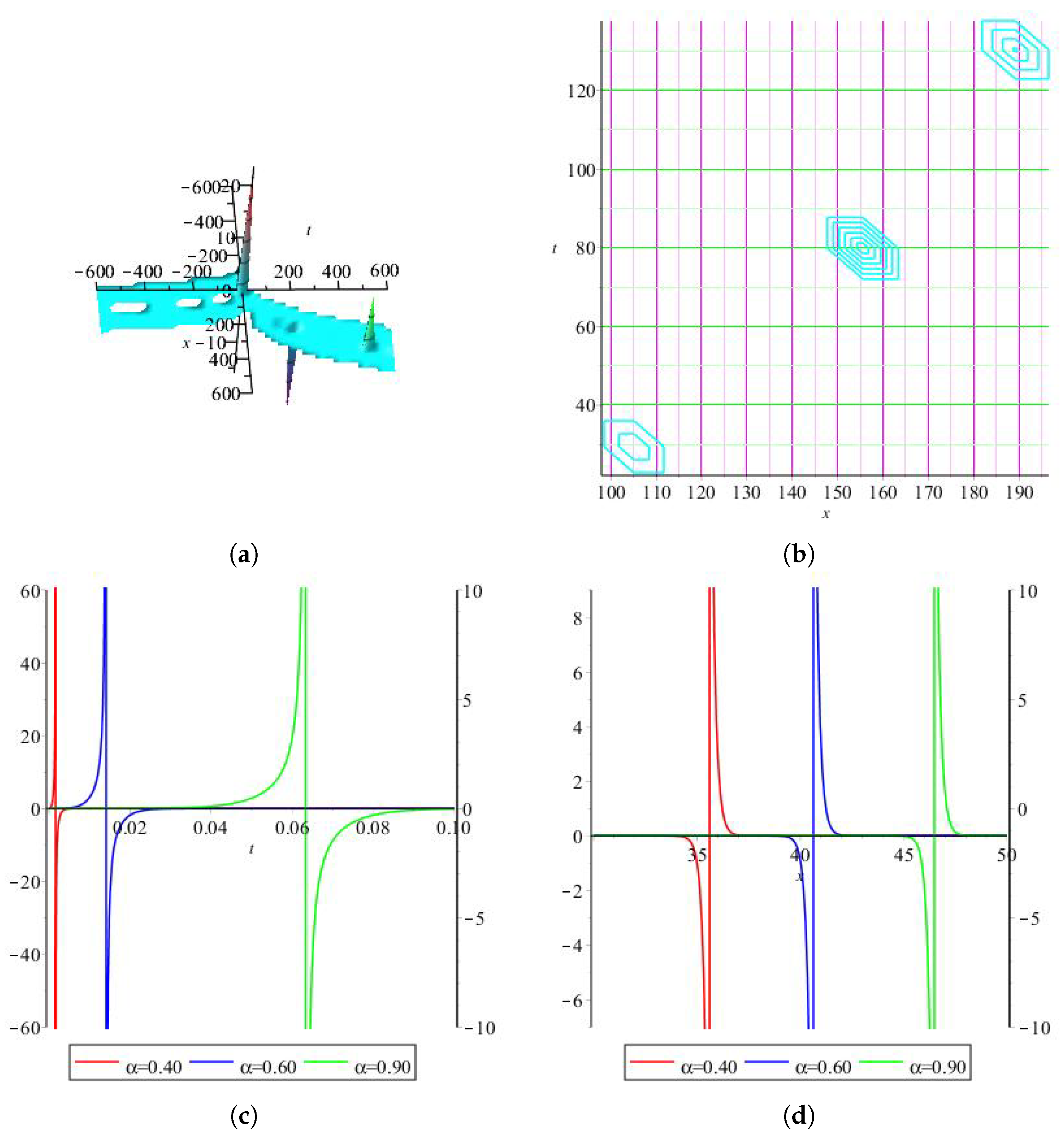
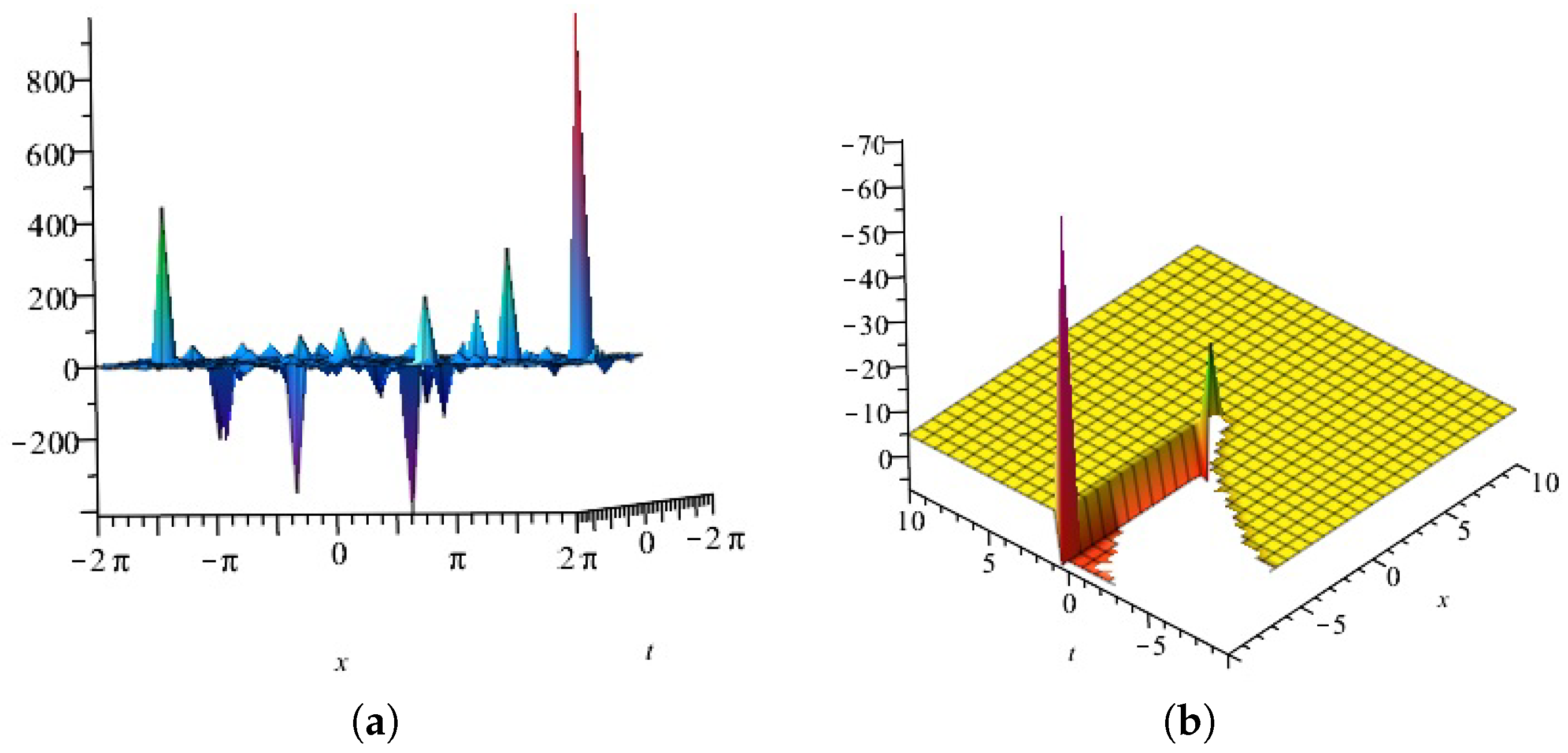
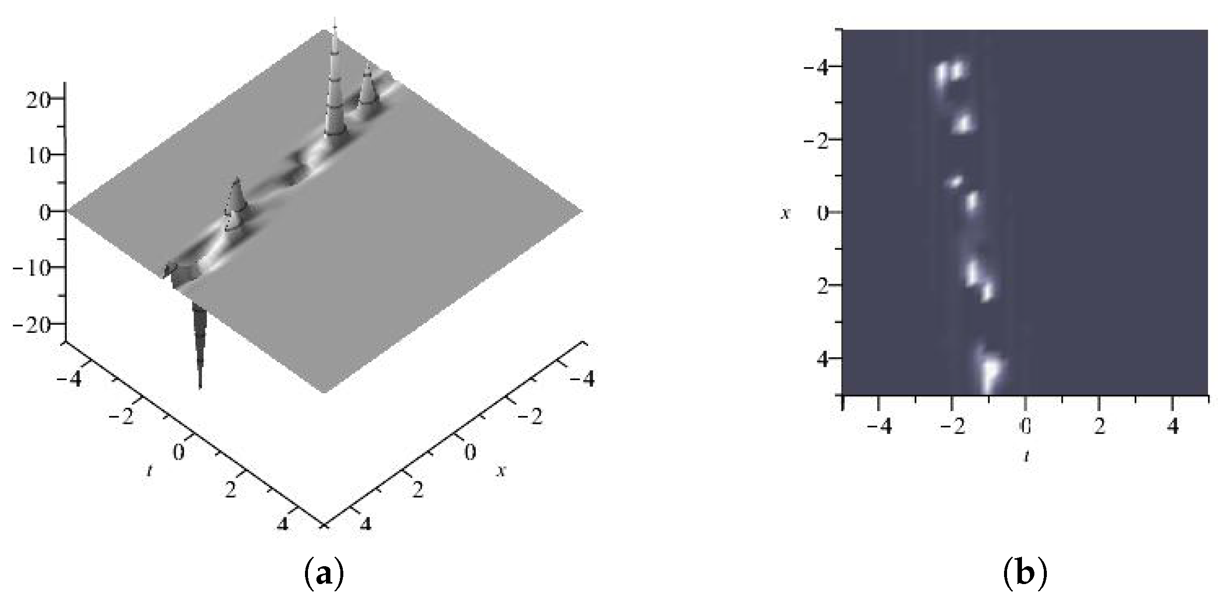
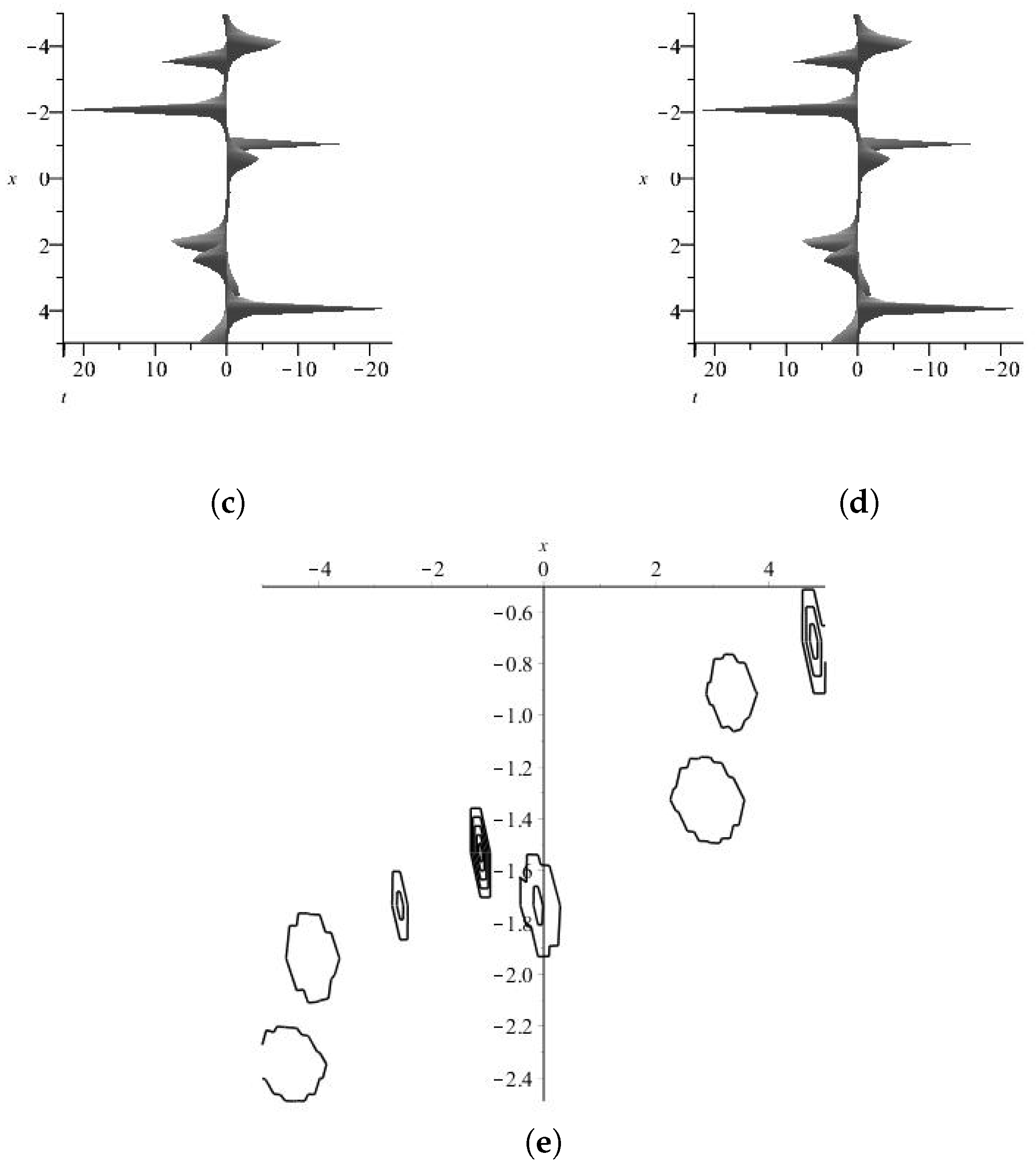
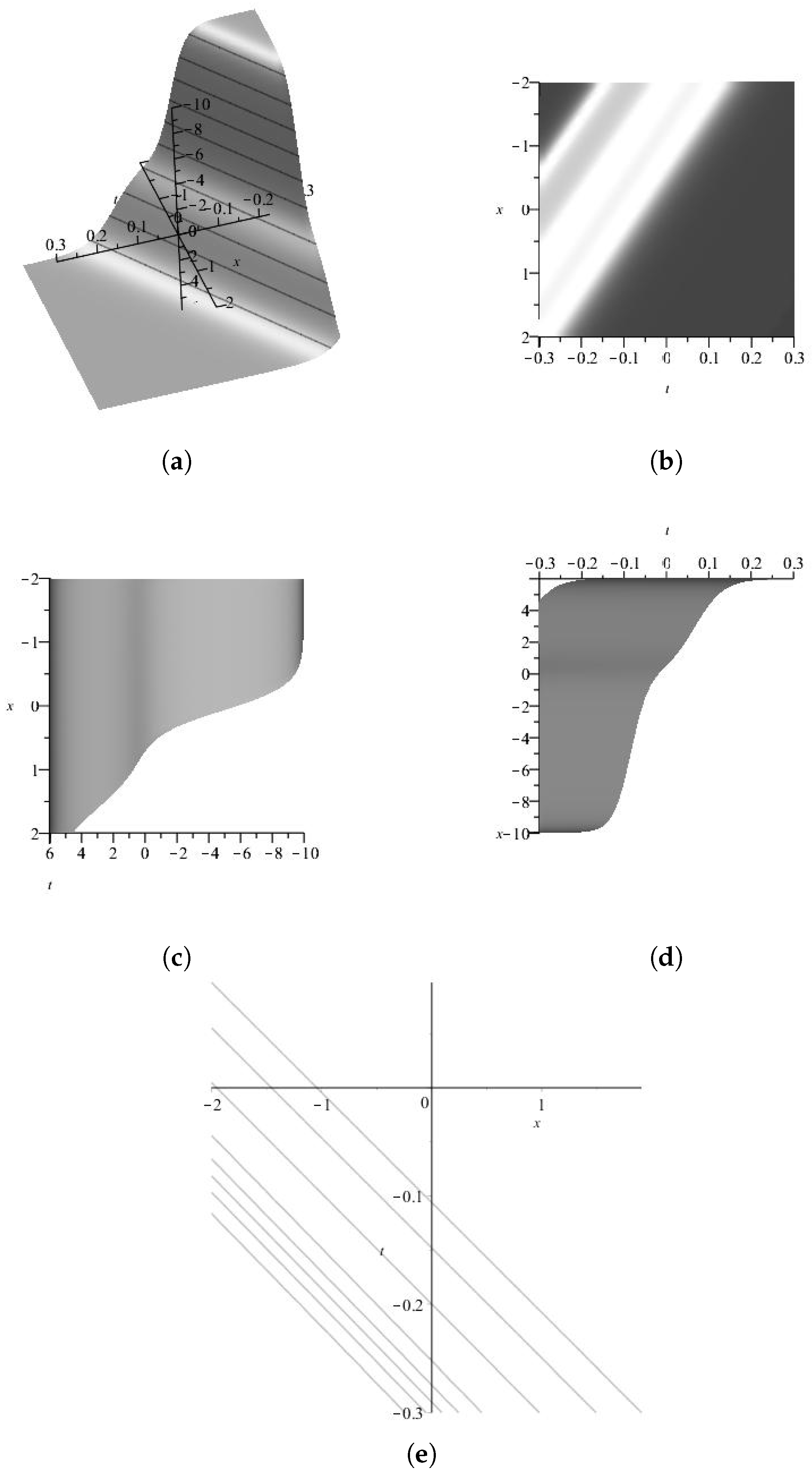
- One wave solutions for (4):First, consider aswhere , and are constants. Now, has the following relationsThe real part of is displayed in Figure 10 for , (a) is three dimensional with Here, (b), (c), and (d) exploit the –axis orientation, respectively. Additionally, (e) is the contour plot. In addition, the imaginary part of equation is displayed in Figure 11 for , (a) is three dimensional with Here, (b), (c), and (d) exploit the –axis, orientation, respectively. Additionally, (e) is the contour plot.
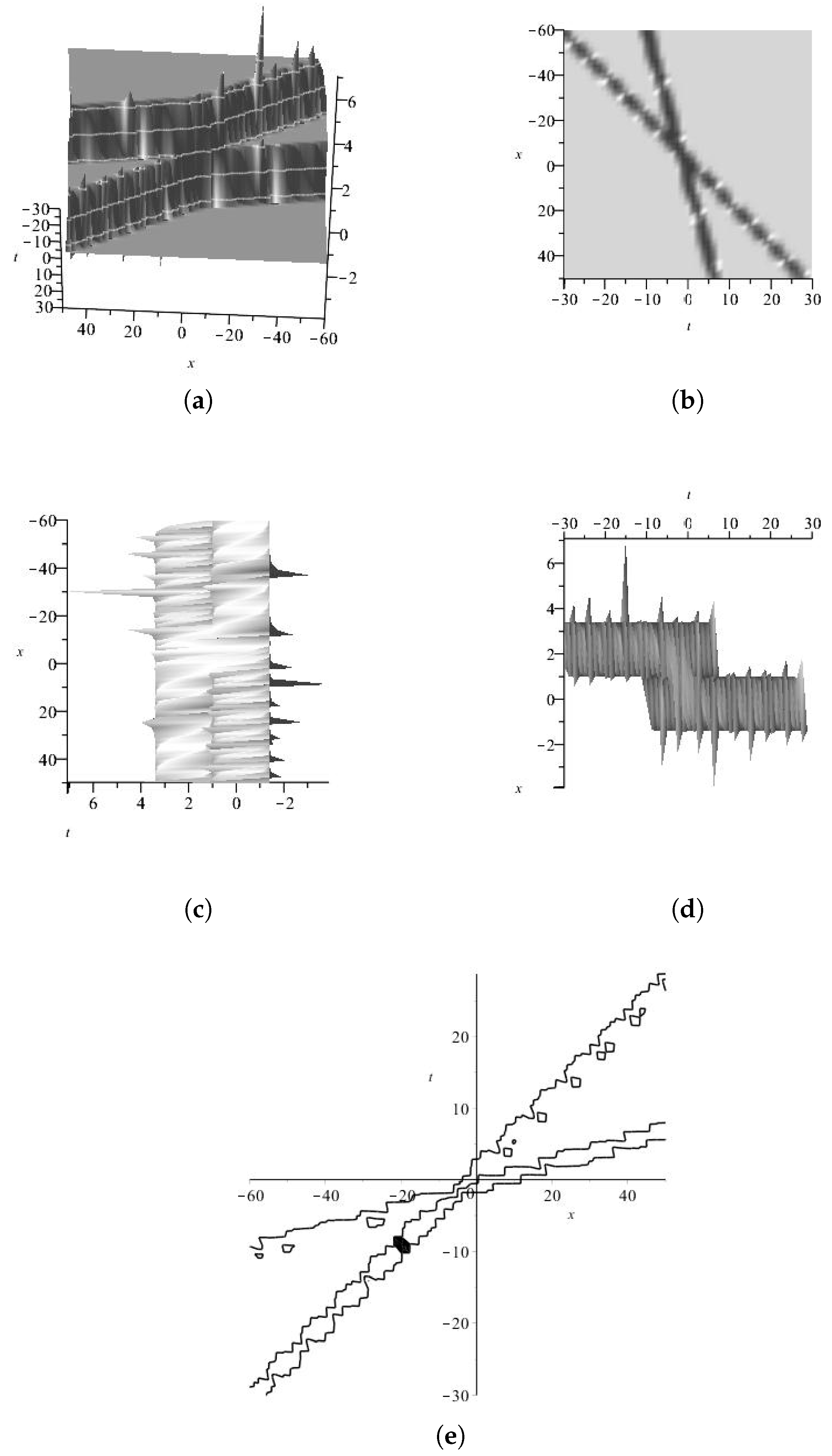
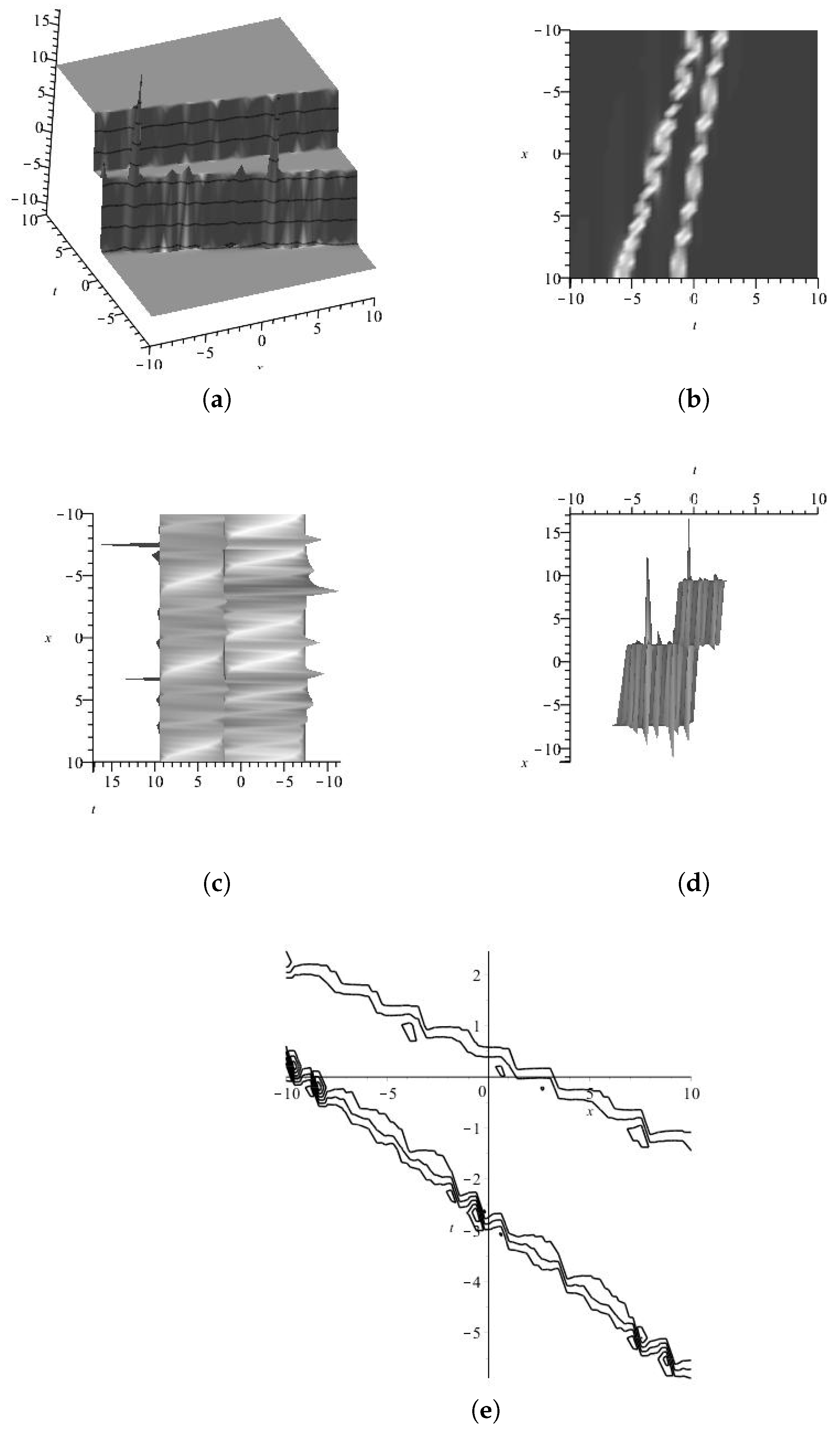
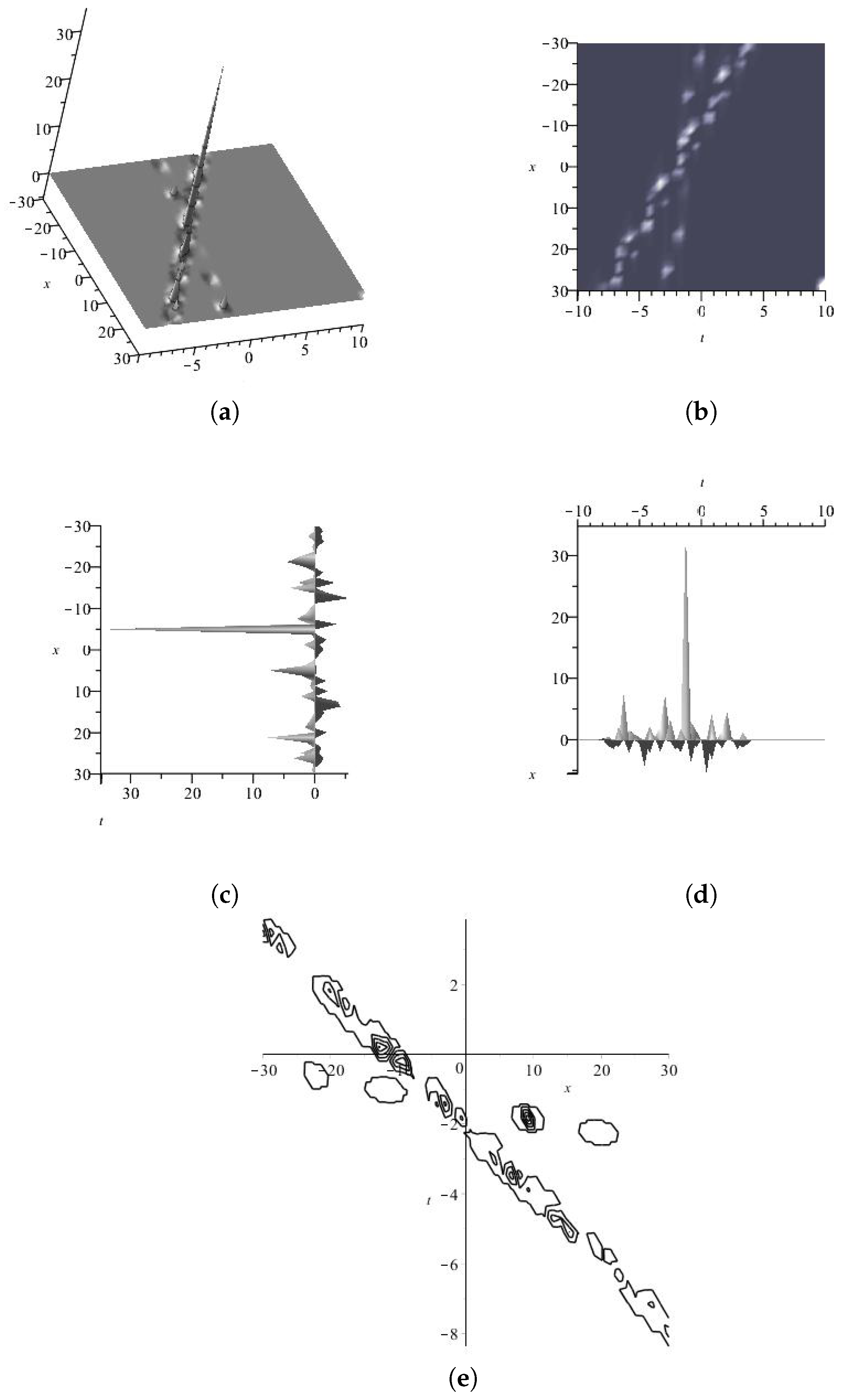
- Two wave solutions for (4):Consider such thatin which and are fixed. Now, we haveUsing (89), we can show that the two wave solutions can be presented by The real part of is displayed in Figure 12 for (a) is three dimensional with Here, (b), (c), and (d) exploit the –axis, respectively. Additionally, (e) is the contour plot. In addition, the imaginary part of equation is displayed in Figure 13 for (a) is three dimensional with Here, (b), (c), and (d) exploit the –axis orientation, respectively. Additionally, (e) is the contour plot.
- Three wave solutions for (4):Consider such thatwhere and are fixed. Now, has the following relationsThus, the three wave solutions can be presented by , respectively.
6.2. Example 2
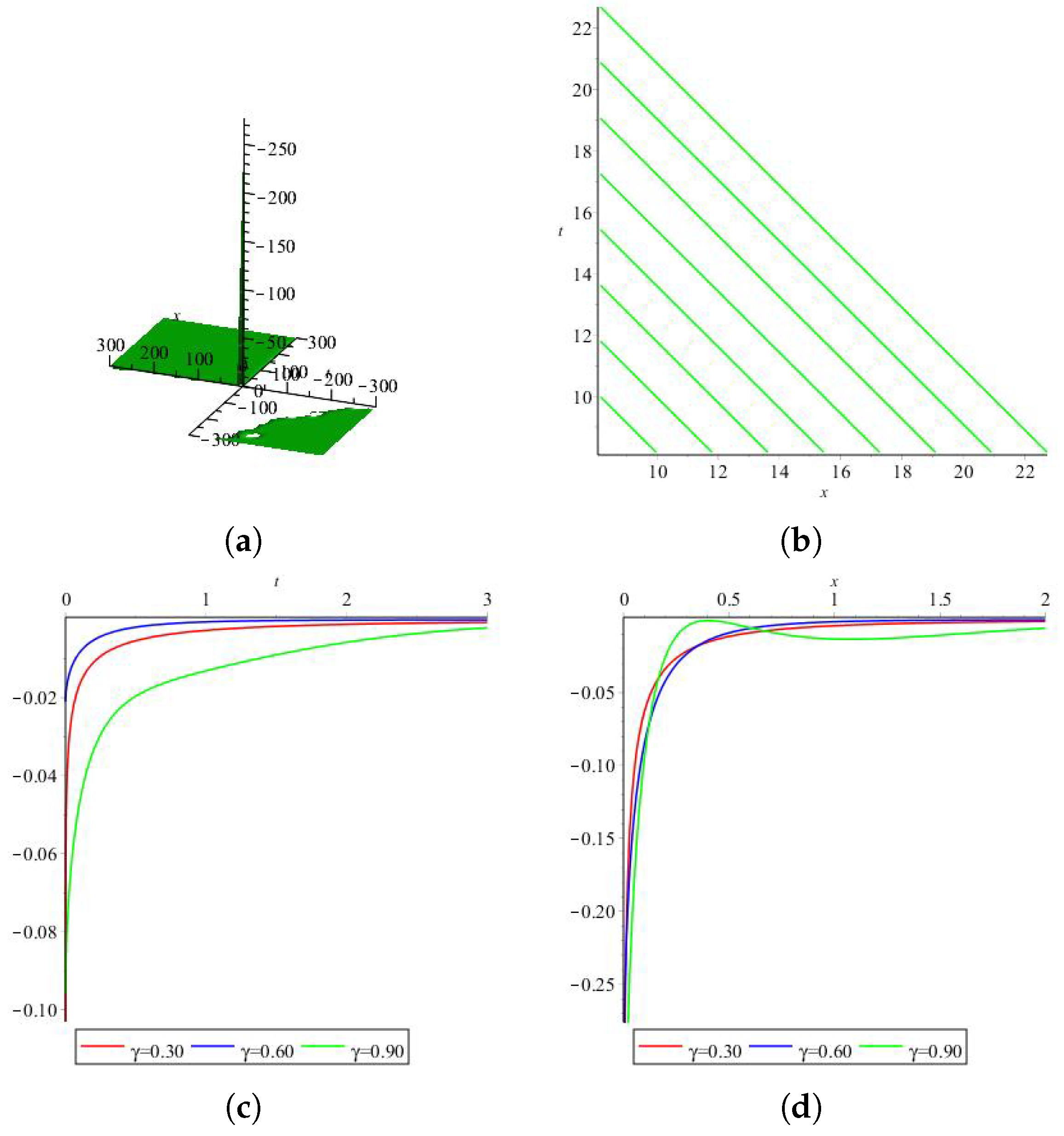
- One wave solutions for (5):In a similar way, we getis displayed in Figure 26 for , (a) is three dimensional with Here, (b), (c), and ( d) exploit the –axis orientation. Additionally, (e) is the contour plot.
- Two wave solutions for (5):In a similar way, we getBy setting the above values in (89), the two wave solutions can be presented byis displayed in Figure 27 for (a) is three dimensional with Here, (b), (c), and (d) exploit the z-axis, y-axis, x-axis orientation, respectively. Additionally, (e) is the contour plot.
- Three wave solutions for (5):In a similar way, we getandThus, the three wave solutions can be presented by respectively.
7. Concluding Remarks
Author Contributions
Funding
Data Availability Statement
Conflicts of Interest
References
- Aderyani, S.R.; Saadati, R.; Vahidi, J.; Allahviranloo, T. The exact solutions of the conformable time-fractional modified nonlinear Schrödinger equation by the Trial equation method and modified Trial equation method. Adv. Math. Phys. 2022, 2022, 4318192. [Google Scholar] [CrossRef]
- Aderyani, S.R.; Saadati, R.; Vahidi, J.; Gómez-Aguilar, J.F. The exact solutions of conformable time-fractional modified nonlinear Schrödinger equation by first integral method and functional variable method. Opt. Quantum Electron. 2022, 54, 218. [Google Scholar] [CrossRef]
- Aderyani, S.R.; Saadati, R.; O’Regan, D.; Alshammari, F.S. Describing Water Wave Propagation Using the G′G–Expansion Method. Mathematics 2022, 11, 191. [Google Scholar] [CrossRef]
- Tarla, S.; Ali, K.K.; Yilmazer, R.; Osman, M.S. New optical solitons based on the perturbed Chen-Lee-Liu model through Jacobi elliptic function method. Opt. Quantum Electron. 2022, 54, 131. [Google Scholar] [CrossRef]
- Yasmin, H.; Aljahdaly, N.H.; Saeed, A.M.; Shah, R. Probing families of optical soliton solutions in fractional perturbed Radhakrishnan–Kundu–Lakshmanan model with improved versions of extended direct algebraic method. Fractal Fract. 2023, 7, 512. [Google Scholar] [CrossRef]
- Aderyani, S.R.; Saadati, R.; Vahidi, J.; Mlaiki, N.; Abdeljawad, T. The exact solutions of conformable time-fractional modified nonlinear Schrödinger equation by Direct algebraic method and Sine-Gordon expansion method. AIMS Math. 2022, 7, 10807–10827. [Google Scholar] [CrossRef]
- Yasmin, H.; Aljahdaly, N.H.; Saeed, A.M.; Shah, R. Investigating Families of Soliton Solutions for the Complex Structured Coupled Fractional Biswas–Arshed Model in Birefringent Fibers Using a Novel Analytical Technique. Fractal Fract. 2023, 7, 491. [Google Scholar] [CrossRef]
- Yasmin, H.; Aljahdaly, N.H.; Saeed, A.M.; Shah, R. Investigating Symmetric Soliton Solutions for the Fractional Coupled Konno–Onno System Using Improved Versions of a Novel Analytical Technique. Mathematics 2023, 11, 2686. [Google Scholar] [CrossRef]
- Hirota, R. The Direct Method in Soliton Theory; No. 155; Cambridge University Press: Cambridge, UK, 2004. [Google Scholar]
- Nguyen, L.T.K. Soliton solution of good Boussinesq equation. Vietnam J. Math. 2016, 44, 375–385. [Google Scholar] [CrossRef]
- Ma, W.X.; Li, C.X.; He, J. A second Wronskian formulation of the Boussinesq equation. Nonlinear Anal. Theory Methods Appl. 2009, 70, 4245–4258. [Google Scholar]
- Nguyen, L.T.K. Wronskian formulation and Ansatz method for bad Boussinesq equation. Vietnam J. Math. 2016, 44, 449–462. [Google Scholar] [CrossRef]
- Behera, S.; Aljahdaly, N.H.; Virdi, J.P.S. On the modified ()-expansion method for finding some analytical solutions of the traveling waves. J. Ocean. Eng. Sci. 2022, 7, 313–320. [Google Scholar] [CrossRef]
- Nadeem, M.; Li, Z.; Alsayyad, Y. Analytical Approach for the Approximate Solution of Harry Dym Equation with Caputo Fractional Derivative. Math. Probl. Eng. 2022, 2022, 4360735. [Google Scholar] [CrossRef]
- Singh, J.; Kumar, D.; Sushila, D. Homotopy perturbation Sumudu transform method for nonlinear equations. Adv. Theor. Appl. Mech. 2011, 4, 165–175. [Google Scholar]
- Ghiasi, E.K.; Saleh, R. A mathematical approach based on the homotopy analysis method: Application to solve the nonlinear Harry-Dym (HD) equation. Appl. Math. 2017, 8, 1546–1562. [Google Scholar] [CrossRef]
- Mokhtari, R. Exact Solutions of the Harry-Dym Equation. Commun. Theor. Phys. 2011, 55, 204. [Google Scholar] [CrossRef]
- Fonseca, F. A Solution of the Harry-Dym Equation Using Lattice-Boltzmannn and a Solitary Wave Methods. Appl. Math. Sci. 2017, 11, 2579–2586. [Google Scholar]
- Rawashdeh, M. A new approach to solve the fractional Harry Dym equation using the FRDTM. Int. J. Pure Appl. Math. 2014, 95, 553–566. [Google Scholar] [CrossRef]
- Iyiola, O.S.; Gaba, Y.U. An analytical approach to time-fractional Harry Dym equation. Appl. Math. Inf. Sci. 2016, 10, 409–412. [Google Scholar] [CrossRef]
- Assabaai, M.A.; Mukherij, O.F. Exact solutions of the Harry Dym Equation using Lie group method. Univ. Aden J. Nat. Appl. Sci. 2020, 24, 481–487. [Google Scholar] [CrossRef]
- Shunmugarajan, B. An Efficient Approach for Fractional Harry Dym Equation by Using Homotopy Analysis Method. Int. J. Eng. Res. Technol. 2016, 5, 561–566. [Google Scholar]
- Al-Khaled, K.; Alquran, M. An approximate solution for a fractional model of generalized Harry Dym equation. Math. Sci. 2014, 8, 125–130. [Google Scholar] [CrossRef]
- Islam, M.T.; Akter, M.A. Distinct solutions of nonlinear space-time fractional evolution equations appearing in mathematical physics via a new technique. Partial Differ. Equ. Appl. Math. 2021, 3, 100031. [Google Scholar] [CrossRef]
- Pavlidou, E.; Papadopoulou, S.K.; Seroglou, K.; Giaginis, C. Revised harris–benedict equation: New human resting metabolic rate equation. Metabolites 2023, 13, 189. [Google Scholar] [CrossRef]
- Perez, V.J.; Leder, R.M.; Badaut, T. Body length estimation of Neogene macrophagous lamniform sharks (Carcharodon and Otodus) derived from associated fossil dentitions. Palaeontol. Electron. 2021, 24, a09. [Google Scholar]
- Liu, A.; Fan, E. On asymptotic stability of multi-solitons for the focusing modified Korteweg–de Vries equation. Phys. D Nonlinear Phenom. 2024, 459, 134046. [Google Scholar] [CrossRef]
- Moretlo, T.S.; Adem, A.R.; Muatjetjeja, B. A generalized (1 + 2)-dimensional Bogoyavlenskii-Kadomtsev-Petviashvili (BKP) equation: Multiple exp-function algorithm; conservation laws; similarity solutions. Commun. Nonlinear Sci. Numer. Simul. 2022, 106, 106072. [Google Scholar] [CrossRef]
- Polyanin, A.D.; Zaitsev, V.F. Handbook of Nonlinear Partial Differential Equations; Chapman and Hall/CRC: Boca Raton, FL, USA, 2016. [Google Scholar]
- Ma, W.X.; Zhu, Z. Solving the (3 + 1)-dimensional generalized KP and BKP equations by the multiple exp-function algorithm. Appl. Math. Comput. 2012, 218, 11871–11879. [Google Scholar]
- Yildirim, Y.; Yaşar, E. Multiple exp-function method for soliton solutions of nonlinear evolution equations. Chin. Phys. B 2017, 26, 070201. [Google Scholar] [CrossRef]
- Adem, A.R. The generalized (1 + 1)-dimensional and (2 + 1)-dimensional Ito equations: Multiple exp-function algorithm and multiple wave solutions. Comput. Math. Appl. 2016, 71, 1248–1258. [Google Scholar] [CrossRef]
- Liu, J.G.; Zhou, L.; He, Y. Multiple soliton solutions for the new (2 + 1)-dimensional Korteweg–de Vries equation by multiple exp-function method. Appl. Math. Lett. 2018, 80, 71–78. [Google Scholar] [CrossRef]
- Zayed, E.M.; Al-Nowehy, A.G. The multiple exp-function method and the linear superposition principle for solving the (2 + 1)-dimensional Calogero–Bogoyavlenskii–Schiff equation. Z. Naturforsch. A 2015, 70, 775–779. [Google Scholar] [CrossRef]
- Long, Y.; He, Y.; Li, S. Multiple soliton solutions for a new generalization of the associated camassa-holm equation by exp-function method. Math. Probl. Eng. 2014, 2014, 418793. [Google Scholar] [CrossRef]
- Aderyani, S.R.; Saadati, R.; Vahidi, J. Multiple exp-function method to solve the nonlinear space–time fractional partial differential symmetric regularized long wave (SRLW) equation and the (1 + 1)-dimensional Benjamin–Ono equation. Int. J. Mod. Phys. B 2022, 37, 2350213. [Google Scholar] [CrossRef]
- Nguyen, L.T.K. Modified homogeneous balance method: Applications and new solutions. Chaos Solitons Fractals 2015, 73, 148–155. [Google Scholar] [CrossRef]


| 0.001 | ±10.8391 | ±5.1739 | ±3.0254 | ±7.9327 | ±0.0069 | ±9.7979 | ±4.9993 | ±4.8005 |
| 0.010 | ±11.4354 | ±3.9987 | ±3.0052 | ±7.9859 | 0.0000 | ±9.7979 | ±4.8991 | ±4.8988 |
| 0.100 | ±15.5875 | ±0.9025 | ±1.6523 | ±14.5247 | 0.0000 | ±9.7979 | ±4.8989 | ±4.8989 |
| 1.001 | ±16.1931 | ±15.2886 | ±9.8816 | ±2.4287 | 0.0000 | ±9.7979 | ±4.8989 | ±4.8989 |
| 1.010 | ±13.5703 | ±10.6300 | ±33.0590 | ±0.7259 | 0.0000 | ±9.7979 | ±4.8989 | ±4.8989 |
| 1.100 | ±18.5057 | ±4.9848 | ±1.4733 | ±13.7668 | 0.0000 | ±9.7979 | ±4.8989 | ±4.8989 |
| 0.001 | 0.0000 | |
| 0.010 | ±4.0050 | 0.0000 |
| 0.100 | ±4.0000 | 0.0000 |
| 1.001 | ±4.0000 | 0.0000 |
| 1.010 | ±4.0000 | 0.0000 |
| 1.100 | ±4.0000 | 0.0000 |
Disclaimer/Publisher’s Note: The statements, opinions and data contained in all publications are solely those of the individual author(s) and contributor(s) and not of MDPI and/or the editor(s). MDPI and/or the editor(s) disclaim responsibility for any injury to people or property resulting from any ideas, methods, instructions or products referred to in the content. |
© 2024 by the authors. Licensee MDPI, Basel, Switzerland. This article is an open access article distributed under the terms and conditions of the Creative Commons Attribution (CC BY) license (https://creativecommons.org/licenses/by/4.0/).
Share and Cite
O’Regan, D.; Aderyani, S.R.; Saadati, R.; Inc, M. Soliton Solution of the Nonlinear Time Fractional Equations: Comprehensive Methods to Solve Physical Models. Axioms 2024, 13, 92. https://doi.org/10.3390/axioms13020092
O’Regan D, Aderyani SR, Saadati R, Inc M. Soliton Solution of the Nonlinear Time Fractional Equations: Comprehensive Methods to Solve Physical Models. Axioms. 2024; 13(2):92. https://doi.org/10.3390/axioms13020092
Chicago/Turabian StyleO’Regan, Donal, Safoura Rezaei Aderyani, Reza Saadati, and Mustafa Inc. 2024. "Soliton Solution of the Nonlinear Time Fractional Equations: Comprehensive Methods to Solve Physical Models" Axioms 13, no. 2: 92. https://doi.org/10.3390/axioms13020092