Article

Numerical Solutions of Second-Order Elliptic Equations with C-Bézier Basis

School of Mathematics and Statistics, Xinyang Normal University, Xinyang 464000, China
*
Author to whom correspondence should be addressed.
Axioms 2024, 13(2), 84; https://doi.org/10.3390/axioms13020084
Submission received: 29 December 2023 / Revised: 18 January 2024 / Accepted: 19 January 2024 / Published: 27 January 2024
(This article belongs to the Topic Numerical Methods for Partial Differential Equations)

Abstract

:
This article introduces a finite element method based on the C-Bézier basis function for second-order elliptic equations. The trial function of the finite element method is set up using a combination of C-Bézier tensor product bases. One advantage of the C-Bézier basis is that it has a free shape parameter, which makes geometric modeling more convenience and flexible. The performance of the C-Bézier basis is searched for by studying three test examples. The numerical results demonstrate that this method is able to provide more accurate numerical approximations than the classical Lagrange basis.

1. Introduction

The finite element method is a powerful numerical tool for solving partial differential equations (PDEs) in the fields of physics [1], mechanics [2], and mathematics [3]. The idea of discrete approximation can be traced back to the ancient practice of partitioning the whole into parts. In 1943, the finite element method was first introduced by Courant [4], who described the unknown functions with piecewise functions on the domain. In the 1960s, Feng [5] demonstrated the convergence of the finite element method. In 1960, Clough [6,7] initially coined and used the term “finite element method” while addressing the elasticity problem. In 1989, Hu [8] established a sufficient and necessary condition for obtaining an energy-rational approximate solution and reported the generalized variational principle of elasticity. Numerous researchers contributed significantly to the development of the finite element approach [9,10,11,12].
The accuracy of the finite element method is increased by a selection of the basis and a suitable mesh refinement. Lagrange [13,14], Bernstein [15], Hermite [16], Argyris [17], and radial basis functions [18] are some classical bases that can be used to construct finite dimensional function spaces. In addition, it has been demonstrated in numerous studies that the finite element method based on spline basis functions is applied to many differential equations, and high precision has been obtained. In 2005, Hughes [19] used the NURBS basis function to conduct a finite analysis after drawing inspiration from Computer Aided Design (CAD). In 2006, Bhatti and Bracken [15] introduced an approach for using a modified Bernstein basis to solve differential equations. In 2010, Zhu [20] presented a numerical solution to the Burgers–Fisher equation based on cubic B-spline quasi interpolation. The numerical results have been compared with the exact solution to illustrate the efficiency of this method. In 2011, Li [21] discretized the elliptic problem by finite elements using the polynomial splines over the hierarchical T-meshes (PHT) spline basis function, and the numerical solution produced a higher order approximation and an effective error estimate. In 2019, a redundant basis was introduced by Kang et al. [22] to solve the Poisson equation numerically. The numerical results show that the error of the spline approximation is identical to that of the standard finite element method. Kacimi et al. [23] provided a Bernstein-Bézier FEM to solve short-wave problems on triangular meshes. In 2020, Peng [24] introduced a Bernstein-Bézier finite element method to simulate the heat transfer process during welding. When the mesh is locally refined, the rational basis function form is used to preserve the accuracy of the geometric shape.
Lagrange, Bernstein, and B-spline basis functions are essentially polynomial or piecewise polynomial basis functions. The intrinsic limitations of these bases, despite their many good qualities, prevent them from accurately portraying several fundamental geometric figures, for example, any quadratic curve other than parabolas or paraboloids. The rational form of the NURBS basis function [25] is unstable, which also increases the complexity of computing integrals and differentials. There have been numerous attempts to create new function spaces [26], but none of these bases can represent higher-order free-form polynomial curves. Accordingly, Wang et al. [26] extended the spaces of mixed algebra and the trigonometric polynomial and proposed a new base, called the C-Bézier basis, for the space T = s p a n 1 , t , , t n 2 , sin t , cos t , in which t n 1 , t n were substituted for sin t and cos t . On the one hand, the C-Bézier basis inherits the desirable properties of the classic Bézier basis function while being an extension of it. On the other hand, the C-Bézier basis has a shape parameter that greatly expands curve and surface modeling and enables the accurate description of arc curves and high-order polynomials. In previous work, scholars obtained good approximate solutions by combining spline functions with the finite element. Spline basis functions have been used to produce better approximations of solutions, as was already discussed, and the C-Bézier basis is a particularly good spline function [27]. Sun et al. [28] showed that the C-Bézier and H-Bézier basis functions have a much better approximation in simulating convection-diffusion problems. Sun et al. [29] combine the Galerkin finite element method with C-Bézier basis functions to solve unsteady elastic equations, and the numerical results indicate that the method has much better precision in solving unsteady elastic equations.
The goal of this paper is to present a numerical approximation method based on the finite element method and C-Bézier basis for solving second-order elliptic equations. Numerical examples are given, and the numerical results indicate that our method has much better precision in solving second-order elliptic equations. The numerical solutions in this paper are generated in MATLAB 2018a. For simplicity, we demonstrate the main idea by considering the following second-order elliptic equation, which seeks an unknown function u ( x , y ) satisfying [30,31]
· ( c u ) = f ( x , y ) , ( x , y ) Ω , u | Ω = g ( x , y ) o n Ω ,
where Ω is a polygonal domain in R 2 , c = ( c i j ( x ) ) 2 × 2 is a symmetric matrix valued function, and g ( x , y ) is the boundary condition of second-order elliptic equation. u is the gradient of u. Assume that a positive constant λ exists such that
λ ξ T ξ ξ T c ξ , ξ R 2 .
Here, ξ is a column vector and ξ T is the transpose of it. In this paper, we apply the C-Bézier basis function to construct the finite dimensional subspace in the finite element method.
The rest of this paper is organized as follows. In Section 2, some notions and preliminary material, such as the Sobolev spaces, norms, and finite element space, will be recalled. In Section 3, we review the definition and excellent properties of the C-Bézier basis function, C-Bézier curves, and tensor product C-Bézier surfaces. In Section 4, we use the C-Bézier basis to construct the trial and test function spaces, and the corresponding C-Bézier finite element method for second-order elliptic equations is given. In Section 5, the error estimates under the L norm, L 2 norm, and H 1 semi-norm are obtained through numerical examples to demonstrate that our scheme improves the efficiency and accuracy of the traditional finite element method compared with Lagrange basis functions. In Section 6, we summarize some comments on the overall work and propose a prospect for the future. This method has the potential to be implemented in higher-dimensional partial differential equations defined on more complex domains.

2. Preliminaries

As a preparation for the finite element algorithm, we briefly present the definitions of Sobolev space H m ( Ω ) and the corresponding norms.
Let Ω R 2 be a bounded domain. The Sobolev space H m ( Ω ) is defined by
H m ( Ω ) = v L 2 ( Ω ) : D γ v L 2 ( Ω ) , if | γ | m ,
with the norm
v H m ( Ω ) = ( | γ | m D γ v L 2 ( Ω ) 2 ) 1 2 ,
and the semi-norm
| v | H m ( Ω ) = ( | γ | = m D γ v | L 2 ( Ω ) 2 ) 1 2 .
In the above equations,
γ = ( γ 1 , γ 2 ) , | γ | = ( γ 1 + γ 2 ) , D γ = | γ | x 1 γ 1 x 2 γ 2 .
For m = 1 , H 0 1 ( Ω ) is the subspace of H 1 ( Ω ) with vanishing boundary values on Ω .
Let Ω h be a partition of Ω ¯ . For each element T Ω h , h T and ρ T are the diameters of T and the largest ball in T, respectively [32]. The mesh size of Ω h is
h = m a x T Ω h h T .
Assume that every element T Ω h has a simplex S ( T ) with diameter
h S ( T ) h .
If there are positive constants c 1 and c 2 that satisfy
m a x T Ω h h T ρ T c 1 , m a x T Ω h m i n T Ω h c 2 ,
the partition Ω h is called quasiuniform.

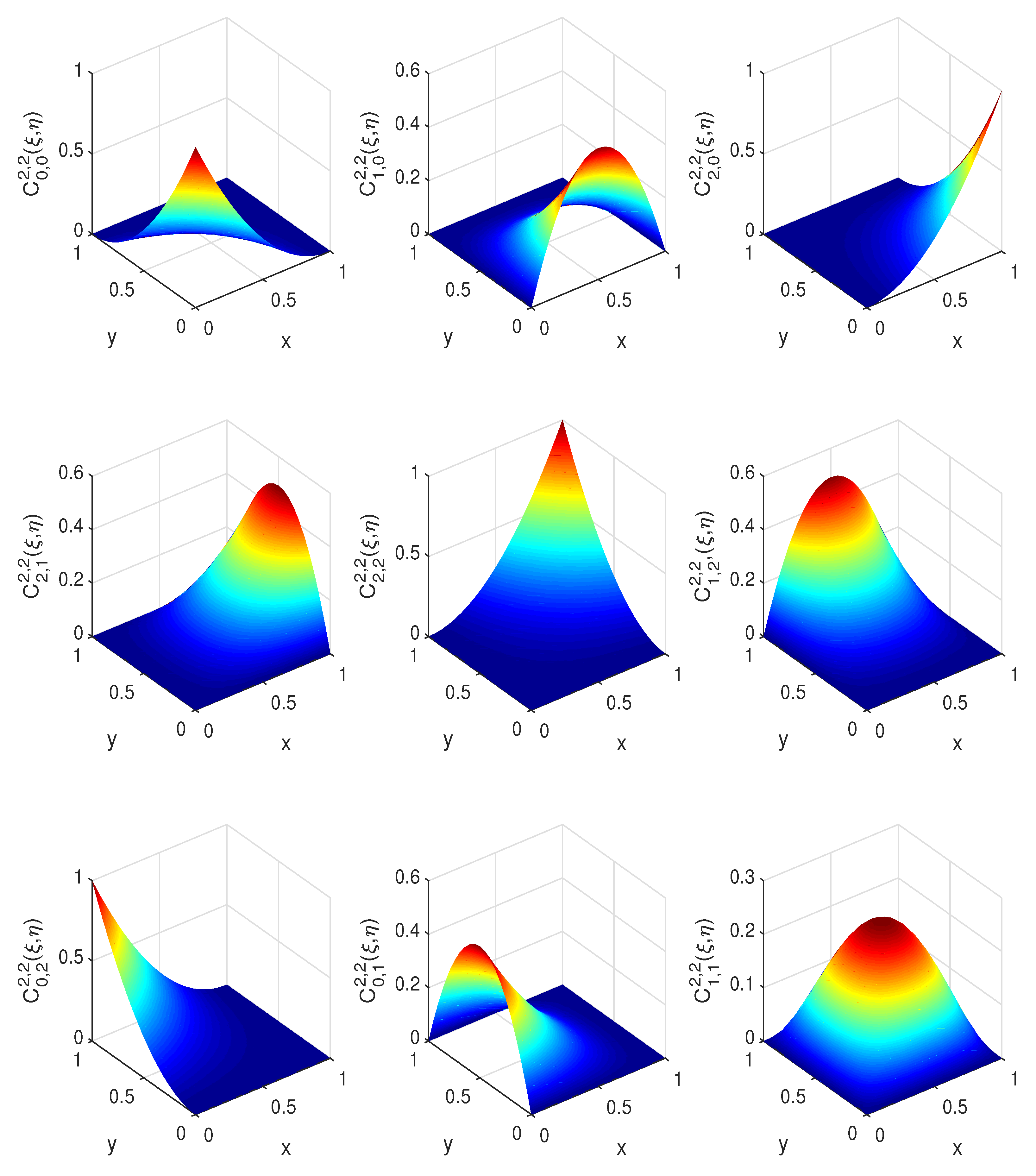
3. C-Bézier Basis, Curve, and Surface

In this section, we recall the definitions and properties of the C-Bézier basis and curves and present corresponding graphs. Furthermore, we generalize the unary C-Bézier basis to the tensor product type and form a kind of tensor product C-Bézier surface.
Definition 1
([26]). The C-Bézier basis C i n ( t ) i = 0 n for the space T = s p a n 1 , t , t n 2 , , sin t , cos t of degrees n is defined by
C 0 n ( t ) = 1 0 t δ 0 n 1 C 0 n 1 ( s ) d s , C i n ( t ) = 0 t δ i 1 n 1 C i 1 n 1 ( s ) d s 0 t δ i n 1 C i n 1 ( s ) d s , i = 1 , 2 , , n 1 , C n n ( t ) = 0 t δ n 1 n 1 C n 1 n 1 ( s ) d s ,
where t [ 0 , α ] , α ( 0 , π ] , n 2 , C 0 1 ( t ) = sin ( α t ) sin α , C 1 1 ( t ) = sin t sin α , δ i n = ( 0 α C i n ( t ) d t ) 1 , and α denotes the length of interval. In addition, α denotes the length of α, which is referred to as the shape parameter. The mathematical expressions of the quadratic C-Bézier basis are as follows, and the graphs generated by Matlab on [ 0 , α ] are shown in Figure 1.
C 0 2 ( t ) = 1 cos ( α t ) 1 cos α , C 1 2 ( t ) = 1 cos t + cos α cos ( α t ) 1 cos α , C 2 2 ( t ) = 1 cos t 1 cos α ,
where t [ 0 , α ] , α ( 0 , π ] . The shape of the C-Bézier basis can be changed by varying the shape parameter α; Figure 1a gives the quadratic C-Bézier basis with α = π 4 , and Figure 1b presents the cubic C-Bézier basis with α = π .
Figure 1. C-Bézier basis functions.
Axioms 13 00084 g001
C-Bézier basis functions are a generalization of classical Bernstein basis functions that pose a lot of common properties, such as affine invariance, endpoints interpolation, convex hull property; all of these properties can be found in [26]. From the graph above, we can see that the C-Bézier basis functions have symmetry, which is written by the mathematical formula as
C i n ( t ) = C n i n ( α t ) f o r t [ 0 , α ] , i = 0 , 1 , , n .
Definition 2
([26]). A C-Bézier curve P ( t ) with control points P i ( x , y , z ) R 3 is defined by
P ( t ) = i = 0 n P i C i n ( t ) ,
where C i n ( t ) is the C-Bézier basis of n degrees, and α is a global shape parameter. The n-sided polygon obtained by connecting two adjacent control vertices with straight segments is called a control polygon.
In the image below, Figure 2a presents a cubic C-Bézier curve with α = π 4 and P i i = 0 3 = ( 0 , 4 ) , ( 1 , 0 ) , ( 2 , 0 ) , ( 4 , 4 ) R 2 . Figure 2b displays a quartic C-Bézier curve with α = π 3 and P i i = 0 4 = ( 0 , 0 ) , ( 2 , 4 ) , ( 4 , 7 ) , ( 6 , 4 ) , ( 8 , 1 ) R 2 . Figure 2c is a quartic C-Bézier curve with α = π 6 and P i i = 0 4 = ( 0 , 0 , 1 ) , ( 1 , 0 , 1 ) , ( 1 , 1 , 1 ) , ( 1 , 1 , 0 ) , ( 0 , 1 , 0 ) R 3 .
The basis of bivariate tensor product spaces is obtained form the tensor product of unary basis functions. For unitary C-Bézier basis functions C i n ( u ) i = 0 m , C j n ( v ) j = 0 n of m and n degrees, the bivariate tensor-product C-Bézier basis of m × n is as follows:
C i , j m , n ( u , v ) = C i m ( u ) C j n ( v ) , i = 0 , 1 , , m , j = 0 , 1 , , n .
Definition 3.
A C-Bézier surface S ( u , v ) of m × n degrees with control points P i , j ( x , y , z ) R 3 is defined by
S ( u , v ) = i = 0 m j = 0 n P i , j C i , j m , n ( u , v ) , ( u , v ) [ 0 , α ] × [ 0 , β ] ,
where C i , j m , n ( u , v ) = C i m ( u ) C j n ( v ) is the tensor-product C-Bézier basis, and α , β are global shape parameters. The grid of m × n edge broken line obtained by connecting two adjacent control vertices in the same row and column with straight segments is called the control grid.
Figure 3 shows two C-Bézier surfaces and their control grids. Study [26] provided several properties of tensor-product C-Bézier surfaces. Here, we will only elaborate on the following three points:
Property 1.
Corner interpolation
At the corners, the C-Bézier surface has the same corner interpolation properties as the Bézier surface. That is,
S ( 0 , 0 ) = P 0 , 0 , S ( 0 , β ) = P 0 , n , S ( α , 0 ) = P m , 0 , S ( α , β ) = P m , n .
Property 2.
Symmetry
S ( α u , β v ) = i = 0 m j = 0 n P i , j C i m ( α u ) C j n ( β v ) = k = 0 m l = 0 n P i , j C k m ( u ) C l n ( v ) = S ( u , v ) , ( u , v ) [ 0 , α ] × [ 0 , β ] .
Property 3.
Partial derivative
k u k S ( u , v ) = i = 0 m k j = 0 n i k P i , j C i m k ( u ) C j n ( v ) l v l S ( u , v ) = i = 0 m j = 0 n l j l P i , j C i m ( u ) C j n l ( v ) k + l u k v l S ( u , v ) = i = 0 m k j = 0 n l j t ( i s P i , j ) C i m k ( u ) C j n l ( v ) , ( u , v ) [ 0 , α ] × [ 0 , β ]
The difference operator is defined by the following recursive formula:
i 0 P i , j = P ( i + 1 , j ) P ( i , j ) i l P i , j = δ i m 1 i 0 P i , j i s P i , j = δ i m s ( i s 1 P i , j ) , s = 1 , 2 , , k , i = 0 , 1 , , m s ,
j 0 P i , j = P ( i , j + 1 ) P ( i , j ) j l P i , j = δ j n 1 j 0 P i , j j t P i , j = δ j n t ( j t 1 P i , j ) , t = 1 , 2 , , l , j = 0 , 1 , , n t ,

4. C-Bézier Finite Element Schemes

This section aims to illustrate how the C-Bézier basis be used in the design of the finite element scheme. With the Dirichlet boundary, the weak formulation of Equation (1) finds u ( x , y ) H 1 ( Ω ) such that u ( x , y ) = g ( x , y ) on Ω and
( c u , v ) = ( f , v ) , v H 0 1 ( Ω ) ,
where ( · , · ) expresses the L 2 -inner product [33,34]. We consider Ω = [ 0 , 1 ] × [ 0 , 1 ] , which is partitioned by a uniform rectangular mesh, denoted by Ω h . Suppose that Ω h is quasiuniform, and mesh size h = [ h 1 , h 2 ] = [ 1 N 1 , 1 N 2 ] , where N 1 , N 2 represent the number of subintervals uniformly divided in x-axis and y-axis. Firstly, we recommend the reference C-Bézier basis of m n degrees on the reference element T ^ = A 1 ^ A 2 ^ A 3 ^ A 4 ^ , where A 1 ^ = ( 0 , 0 ) , A 2 ^ = ( 1 , 0 ) , A 3 ^ = ( 1 , 1 ) , and A 4 ^ = ( 0 , 1 ) .
The tensor product C-Bézier basis of m n degrees on element [ 0 , α ] × [ 0 , β ] is
C i , j m , n ( x ^ , y ^ ) = C i m ( x ^ ) C j n ( y ^ ) , i = 0 , , m , j = 0 , n .
Let ξ = x ^ α , η = y ^ β ; then, the reference C-Bézier basis as follows:
C i , j m , n ( ξ , η ) = C i m ( α ξ ) C j n ( β η ) , i = 0 , , m , j = 0 , n ,
where ( ξ , η ) [ 0 , 1 ] × [ 0 , 1 ] . Plots of nine reference biquadratic C-Bézier bases with α = β = π 6 are shown in Figure 4.
Subsequently, we can use the affine mapping between the reference element and an arbitrary element to obtain the local basis functions. For an element T Ω h , denote the local finite element space by W ( T , m , n ) , i.e.,
W ( T , m , n ) = v , v s p a n C i , j m , n ( x , y ) i , j = 0 m , n , ( x , y ) T . .
Then, a finite dimensional space would be constructed by patching W ( T , m , n ) over all the elements T Ω h . That is, the finite element space can be written as [35]
U h ( m , n ) = v , v W ( T , m , n ) , T Ω h .
The space U h 0 ( m , n ) is the subspace of U h ( m , n ) containing the functions that vanish on the boundary of domain Ω , i.e.,
U h 0 ( m , n ) = v U h , v | T Ω = 0 , T Ω h .
For any u , v U h ( m , n ) , we introduce a bilinear form as follows:
a ( u , v ) = ( c u , v ) ,
where ( c u , v ) = Ω c u · v d Ω .
Finite Element Algorithm . An approximation for Equation ( 1 ) can be obtained by finding u h U h ( m , n ) satisfying u h | Ω = g h and
a ( u h , v h ) = ( f , v h ) , v h U h 0 ( m , n ) .
where g h is an discretization of the boundary value u ( x , y ) = g ( x , y ) at the finite element nodes. The steps of above method is shown in the folowing Algorithm 1.
Algorithm 1 Steps of finite element method with C-Bézier basis functions
Step 1: 
Initialization: Specify the elliptic Equation (1) to be solved and the associated boundary conditions.
Step 2: 
Establish a weak form (12): multiply both sides of the equation by the C-Bézier basis function and integrate over the solution domain.
Step 3: 
In order to take advantage of the boundary conditions, deal with the integral using Green’s formula.
Step 4: 
Update the weak form: Place the terms with unknowns on the left side to form an algebraic system.
Step 5: 
Solve algebraic systems to obtain approximate solutions for unknowns.
Step 6: 
Verify the correctness of the numerical solution, and carry out error analysis and visualization.

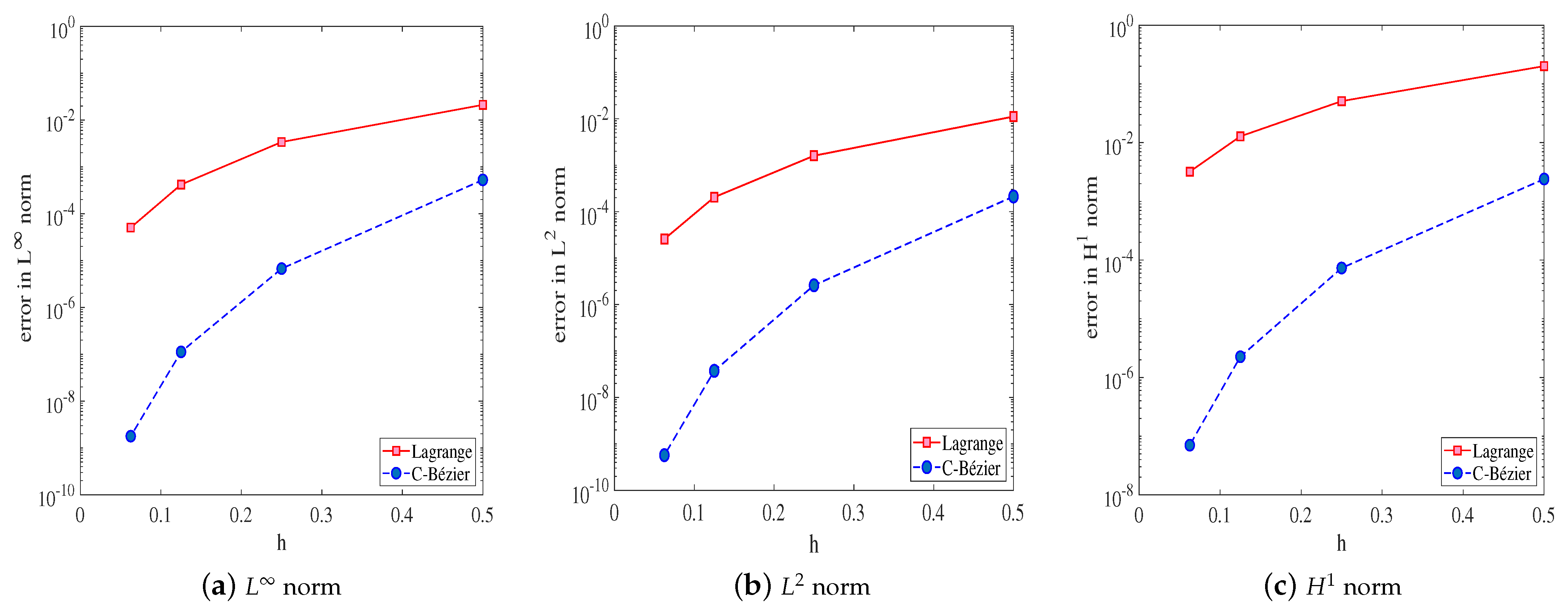
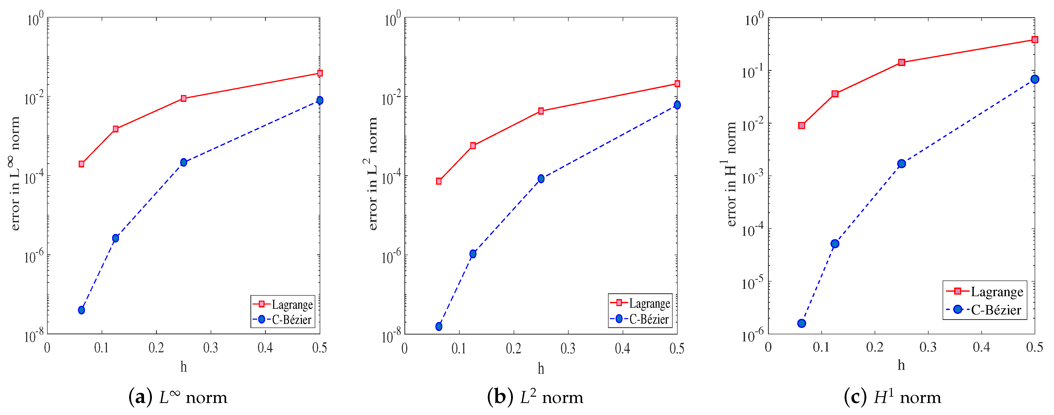
5. Approximation of Solutions with the C-Bézier Basis

In this section, three numerical experiments will be implemented to see the performance of the C-Bézier basis method. The approximate solutions are solved by MATLAB software; in all experiments, Ω is divided by quasiuniform rectangle meshes. The results of the suggested algorithm will be compared with those obtained with the Lagrange basis in terms of three error norms [36,37]:
u u h = s u p x Ω | u u h | ( L n o r m e r r o r ) ,
u u h 0 = Ω ( u u h ) 2 d x d y ( L 2 n o r m e r r o r ) ,
| u u h | 1 = Ω ( u u h ) x 2 d x d y + Ω ( u u h ) y 2 d x d y
( H 1 s e m i n o r m e r r o r ) .
Example 1.
Consider the equation
· ( u ) = 2 π 2 sin ( π x ) sin ( π y ) , ( x , y ) Ω , u | Ω = 0
where Ω = [ 0 , 1 ] × [ 0 , 1 ] ; the exact solution is
u ( x , y ) = sin ( π x ) sin ( π y ) .
In the following, we use the finite element method with the tensor product biquadratic C-Bézier and Lagrange basis to seek the numerical solutions and calculate the error norms on Guass points.
To illustrate, mesh size h = [ h 1 , h 2 ] . In Table 1 and Figure 5, it can be observed that the numerical solutions derived by the C-Bézier basis are 2–4 orders of magnitude more accurate than that of the Lagrange basis. This indicates that the C-Bézier finite element method works well for elliptic problems involving Dirichlet boundary conditions applied on edges. Figure 6 shows the L norm errors of the Lagrange basis and the C-Bézier basis function with h = [ 1 4 , 1 4 ] .
Example 2.
The second-order elliptic equation with Dirichlet boundary conditions is given as
· ( u ) = 2 π 2 sin ( π x ) cos ( π x ) ( 3 sin 2 ( π y ) cos 2 ( π y ) ) , ( x , y ) Ω , u | Ω = 0
where Ω = [ 0 , 1 ] × [ 0 , 1 ] . The exact solution of ( 15 ) is
u ( x , y ) = sin ( π x ) cos ( π x ) sin 2 ( π y ) .
Similar to Example 1, the finite element method and C-Bézier basis are used to solve Equation ( 15 ) .
Table 2 and Figure 7 demonstrate that, when the Lagrange basis and C-Bézier basis function reaches the same convergence order, the mesh size of the latter is more refined. This means that the C-Bézier finite element method function not only reduces the computing complexity but also improves the precision of the numerical solution significantly compared with the Lagrange basis with the same mesh size. When h = [ 1 4 , 1 4 ] , the graph of the errors in the L norm is depicted in Figure 8.
Example 3.
Consider another second-order elliptic equation
· ( u ) = 5 4 π 2 sin ( π x ) cos ( π y 2 ) , ( x , y ) Ω , u | Ω = 0
where Ω = [ 0 , 1 ] × [ 1 , 3 ] . The exact solution of ( 16 ) is
u ( x , y ) = sin ( π x ) cos ( π y 2 ) .
The errors obtained with the C-Bézier and Lagrange basesin L norm, L 2 norm, and H 1 semi-norm are shown in Table 3 and Figure 9. The single most striking observation to emerge from the data comparison is that the precision of numerical solutions obtained by the traditional Lagrange basis is 1 4 orders of magnitude lower than that of the C-Bézier basis, which suggests that the C-Bézier finite element method works better than the Lagrange basis. Figure 10 provides the error in L norm pictures of Lagrange and C-Bézier with h = [ 1 4 , 1 2 ] .

6. Conclusions and Further Work

This essay presents a detailed finite element algorithm description of how the C-Bézier basis can be applied to give more accurate solutions for second-order elliptic equations in two-dimensional space. One of the most significant findings to emerge from this study is that the accuracy of numerical solutions obtained by the C-Bézier basis is 1–4 orders of magnitude higher than that of the Lagrange basis. The major limitation of this study is the inability to theoretically determine the value of the optimal shape parameter α .
There are several interesting questions worth exploring further. Firstly, elliptic equations with different boundary conditions, including Neumann and Robin boundary conditions can be solved using the C-Bézier finite element method. Secondly, the C-Bézier finite method can probably be extended to the calculation of other models, such as parabolic equations, hyperbolic equations, and coupled partial differential equations in three-dimensional space.

Author Contributions

L.S. carried out the program and conceived the paper. F.S. and K.P. helped to draft and revise the manuscript. L.S., F.S. and K.P. supplied significant information about current research to the introduction and conclusion. All authors have read and agreed to the published version of the manuscript.

Funding

This work is partly supported by Program for Science Technology Innovation Talents in Universities of Henan Province (No. 22HASTIT021), the Science and Technology Project of Henan Province (No. 212102210394), and the Graduate Innovation Project of Xinyang Normal University (No. 2021KYJJ48).

Data Availability Statement

Data are contained within the article.

Acknowledgments

The authors are very grateful to the editor and anonymous referees for their valuable comments and constructive suggestions, which helped to improve the paper significantly.

Conflicts of Interest

The authors declare no conflict of interest.

References

  1. Xu, F. A Cascadic Adaptive Finite Element Method for Nonlinear Eigenvalue Problems in Quantum Physics. Multiscale Model. Simul. 2020, 18, 198–220. [Google Scholar] [CrossRef]
  2. Arora, R.; Zhang, X.; Acharya, A. Finite element approximation of finite deformation dislocation mechanics. Comput. Methods Appl. Mech. Eng. 2020, 367, 113076. [Google Scholar] [CrossRef]
  3. Fu, G.; Xu, Z. High-order space-time finite element methods for the Poisson-Nernst-Planck equations: Positivity and unconditional energy stability. Comput. Methods Appl. Mech. Eng. 2021, 395, 115031. [Google Scholar] [CrossRef]
  4. Courant, R. Variational Methods for the Solution of Problems of Equilibrium and Vibration. Bull. Am. Math. Soc. 1943, 49, 1–23. [Google Scholar] [CrossRef]
  5. Feng, K. Difference scheme based on variational principle. Appl. Comput. Math. 1965, 2, 238–262. [Google Scholar]
  6. Clough, R.L. Thoughts about the origin of the finite element method. Comput. Struct. 2001, 79, 2029–2030. [Google Scholar] [CrossRef]
  7. Clough, R.L. Early history of the finite element method from the view point of a pioneer. Int. J. Numer. Meth. Eng. 2004, 60, 283–287. [Google Scholar] [CrossRef]
  8. Hu, H. Correct application of generalized variational principle of elasticity to approximate solution. Siam. J. Multiscale. Model. Sim. 1989, 19, 1159–1166. [Google Scholar]
  9. Clough, R.W. The Finite Element Method in Plane Stress Analysis. In Proceedings of the Asce Conference on Electronic Computation, Pittsburgh, PA, USA, 8–10 September 1960. [Google Scholar]
  10. Babuka, I. Error-bounds for finite element method. Numer. Math. 1971, 16, 322–333. [Google Scholar] [CrossRef]
  11. Li, H.; Wang, D.; Song, Z.; Zhang, F. Numerical analysis of an unconditionally energy-stable reduced-order finite element method for the Allen-Cahn phase field model. Comput. Math. Appl. 2021, 96, 67–76. [Google Scholar] [CrossRef]
  12. Kawecki, E.L. Finite element theory on curved domains with applications to discontinuous Galerkin finite element methods. Numer. Methods Partial. Differ. Equ. 2020, 36, 1492–1536. [Google Scholar] [CrossRef]
  13. Csati, Z.; Moes, N.; Massart, T.J. A stable extended/generalized finite element method with Lagrange multipliers and explicit damage update for distributed cracking in cohesive materials. Comput. Methods Appl. Mech. Eng. 2020, 369, 113173. [Google Scholar] [CrossRef]
  14. Alcntara, A.A.; Carmo, B.A.; Clark, H.R.; Guardia, R.R.; Rincon, M.A. On a nonlinear problem with Dirichlet and Acoustic boundary conditions. Appl. Math. Comput. 2021, 411, 126514–126533. [Google Scholar] [CrossRef]
  15. Bhatti, M.I.; Bracken, B.P. Solutions of differential equations in a Bernstein polynomial basis. J. Comput. Appl. Math. 2007, 205, 272–280. [Google Scholar] [CrossRef]
  16. Tang, Y.; Yin, Z. Hermite Finite Element Method for a Class of Viscoelastic Beam Vibration Problem. Engineering 2021, 13, 463–471. [Google Scholar] [CrossRef]
  17. Ebrahimi, F. A C1 finite element method for axisymmetric lipid membranes in the presence of the Gaussian energy. Comput. Methods Appl. Mech. Eng. 2022, 391, 114472. [Google Scholar] [CrossRef]
  18. Pais, A.I.; Lves, J.L.; Belinha, J. Using a radial point interpolation meshless method and the finite element method for application of a bio-inspired remodelling algorithm in the design of optimized bone scaffold. J. Braz. Soc. Mech. Sci. 2021, 43, 557. [Google Scholar] [CrossRef]
  19. Hughes, T.J.R.; Cottrell, J.A.; Bazilevs, Y. Isogeometric analysis: CAD, finite elements, NURBS, exact geometry and mesh refinement. Engineering 2005, 194, 4135–4195. [Google Scholar] [CrossRef]
  20. Zhu, C.; Kang, W. Numerical solution of Burgers-Fisher equation by cubic B-spline quasi-interpolation. Appl. Math. Comput. 2020, 216, 2679–2686. [Google Scholar] [CrossRef]
  21. Li, T.; Chen, F.; Du, Q. Adaptive finite element methods for elliptic equations over hierarchical T-meshes. J. Comput. Appl. Math. 2011, 236, 878–891. [Google Scholar]
  22. Kang, H.; Lai, M.; Li, X. An economical representation of PDE solution by using compressive sensing approach. Comput.-Aided Des. 2019, 115, 78–86. [Google Scholar] [CrossRef]
  23. Kacimi, A.E.; Ouazar, D.; Mohamed, M.S.; Seaid, M.; Trevelyan, J. Enhanced conformal perfectly matched layers for Bernstein-Bézier finite element modeling of short wave scattering. Engineering 2019, 355, 614–638. [Google Scholar]
  24. Peng, X.; Xu, G.; Zhou, O.; Yang, Y.; Ma, Z. An adaptive Bernstein-Bézier finite element method for heat transfer analysis in welding. Adv. Eng. Softw. 2020, 148, 102855. [Google Scholar] [CrossRef]
  25. Sevilla, R.; Fernández-Méndez, S.; Huerta, A. NURBS-enhanced finite element method (NEFEM). Arch. Comput. Methods Eng. 2011, 18, 441–484. [Google Scholar] [CrossRef]
  26. Chen, Q.; Wang, G. A class of Bézier-like curves. Comput. Aided Geom. Des. 2003, 20, 29–39. [Google Scholar] [CrossRef]
  27. Sun, L.; Su, F. Application of C-Bézier and H-Bézier basis in solving heat conduction problems. J. Xinyang Norm. Univ. (Nat. Sci. Ed.) 2022, 35, 1–6. [Google Scholar]
  28. Sun, L.; Su, F. Application of C-Bézier and H-Bézier basis functions to numerical solution of convection-diffusion equations. Bound. Value. Probl. 2022, 2022, 66. [Google Scholar] [CrossRef]
  29. Sun, L.; Pang, K. Numerical solution of unsteady elastic equations with C-Bézier basis functions. AIMS Math. 2024, 9, 702–722. [Google Scholar] [CrossRef]
  30. Badia, S.; Verdugoand, F.; Alberto, F. The aggregated unfitted finite element method for elliptic problems. Comput. Methods Appl. Mech. Eng. 2021, 336, 533–553. [Google Scholar] [CrossRef]
  31. Guan, Q.; Gunzburger, M.; Zhao, W. Weak-Galerkin finite element methods for a second-order elliptic variational inequality. Comput. Methods Appl. Mech. Eng. 2018, 337, 677–688. [Google Scholar] [CrossRef]
  32. Bramble, J.H.; Xu, J. Some estimates for a weighted L2 projection. Math. Comput. 1991, 56, 463–470. [Google Scholar]
  33. Chen, Z.; Tuo, R.; Zhang, W. A finite element method for elliptic problems with observational boundary data. Comput. Appl. Math. 2020, 38, 355–372. [Google Scholar]
  34. Li, R.; Liu, B. Numerical Solutions for Differential Equations; Academic Press: Cambridge, MA, USA, 1997; pp. 252–253. [Google Scholar]
  35. Wang, J.; Ye, X. A weak Galerkin Finite Element Method for Second-Order Elliptic Problems. J. Comput. Appl. Math. 2013, 241, 103–115. [Google Scholar] [CrossRef]
  36. Coelho, K.O.; Devloo, P.; Gomes, S.M. Error estimates for the Scaled Boundary Finite Element Method. Comput. Math. 2021, 379, 113765. [Google Scholar] [CrossRef]
  37. Chen, Y.; Huang, Y.; Yi, N. Error analysis of a decoupled, linear and stable finite element method for Cahn–Hilliard–Navier–Stokes equations. Appl. Math. Comput. 2022, 421, 126928. [Google Scholar] [CrossRef]
Figure 2. C-Bézier curves with α = π 4 , π 3 and π 6 .
Axioms 13 00084 g002
Figure 3. Tensor-product C-Bézier surfaces and their control grids.
Axioms 13 00084 g003
Figure 4. Reference biquadratic C-Bézier basis.
Axioms 13 00084 g004
Figure 5. Error graphs (generated from Example 1).
Axioms 13 00084 g005
Figure 6. Error graphs.
Axioms 13 00084 g006
Figure 7. Error graphs.
Axioms 13 00084 g007
Figure 8. Error graphs.
Axioms 13 00084 g008
Figure 9. Error graphs (generated from Example 3).
Axioms 13 00084 g009
Figure 10. Error graphs.
Axioms 13 00084 g010
Table 1. The numerical errors for quadratic element of Example 1.
Basis h 1 h 2 α β | | u u h | | | | u u h | | 0 | u u h | 1 CPU Time (s)
Lagrange 1 2 1 2 -- 2.1100 × 10 2 1.1180 × 10 2 2.0120 × 10 1 0.614
1 4 1 4 -- 3.4000 × 10 3 1.6000 × 10 3 5.0900 × 10 2 0.295
1 8 1 8 -- 4.1941 × 10 4 2.0486 × 10 4 1.2800 × 10 2 1.026
1 16 1 16 -- 5.0651 × 10 5 2.5717 × 10 5 3.2000 × 10 3 4.414
C-Bézier 1 2 1 2 π 2 π 2 5.2767 × 10 4 2.1224 × 10 4 2.4000 × 10 3 0.239
1 4 1 4 π 4 π 4 6.7404 × 10 6 2.5977 × 10 6 7.3090 × 10 5 0.285
1 8 1 8 π 8 π 8 1.1237 × 10 7 3.7353 × 10 8 2.2559 × 10 6 1.050
1 16 1 16 π 16 π 16 1.7821 × 10 9 5.7064 × 10 10 7.0261 × 10 8 4.316
Table 2. The numerical errors for the quadratic element of Example 2.
Basis h 1 h 2 α β | | u u h | | | | u u h | | 0 | u u h | 1 CPU Time (s)
Lagrange 1 2 1 2 -- 3.8500 × 10 2 2.1000 × 10 2 3.8290 × 10 1 0.209
1 4 1 4 -- 8.9000 × 10 3 4.3000 × 10 3 1.4130 × 10 1 0.321
1 8 1 8 -- 1.5000 × 10 3 5.7229 × 10 4 3.5900 × 10 2 1.236
1 16 1 16 -- 1.9614 × 10 4 7.2516 × 10 5 9.0000 × 10 3 4.226
C-Bézier 1 2 1 2 π π 7.9000 × 10 3 6.1000 × 10 3 6.7900 × 10 2 0.084
1 4 1 4 π 2 π 2 2.1516 × 10 4 8.3757 × 10 5 1.7000 × 10 3 0.345
1 8 1 8 π 4 π 4 2.6147 × 10 6 1.0609 × 10 6 5.1633 × 10 5 1.152
1 16 1 16 π 8 π 8 3.9968 × 10 8 1.5542 × 10 8 1.5946 × 10 6 4.339
Table 3. The numerical errors for quadratic element of Example 3.
Basis h 1 h 2 α β | | u u h | | | | u u h | | 0 | u u h | 1 CPU Time (s)
Lagrange 1 2 1 -- 2.0000 × 10 2 1.6400 × 10 2 2.2480 × 10 1 0.227
1 4 1 2 -- 3.3000 × 10 3 2.3000 × 10 3 5.6900 × 10 2 0.291
1 8 1 4 -- 4.1473 × 10 4 2.8968 × 10 4 1.4300 × 10 2 1.123
1 16 1 8 -- 5.0648 × 10 5 3.6369 × 10 6 3.6000 × 10 3 4.243
C-Bézier 1 2 1 π 2 π 2 4.9460 × 10 4 2.8379 × 10 4 2.7000 × 10 3 0.076
1 4 1 2 π 4 π 4 6.6507 × 10 6 3.6257 × 10 6 8.1731 × 10 5 0.287
1 8 1 4 π 8 π 8 1.1203 × 10 7 5.2667 × 10 8 2.5221 × 10 6 1.059
1 16 1 8 π 16 π 16 1.7808 × 10 9 8.0642 × 10 10 7.8554 × 10 8 4.459
Disclaimer/Publisher’s Note: The statements, opinions and data contained in all publications are solely those of the individual author(s) and contributor(s) and not of MDPI and/or the editor(s). MDPI and/or the editor(s) disclaim responsibility for any injury to people or property resulting from any ideas, methods, instructions or products referred to in the content.

