
Boolean Subtypes of the U4 Hexagon of Opposition


1
Center for Logic and Philosophy of Science, KU Leuven, 3000 Leuven, Belgium
2
KU Leuven Institute for Artificial Intelligence, KU Leuven, 3000 Leuven, Belgium
*
Author to whom correspondence should be addressed.
Axioms 2024, 13(2), 76; https://doi.org/10.3390/axioms13020076
Submission received: 24 December 2023
/
Revised: 19 January 2024
/
Accepted: 22 January 2024
/
Published: 24 January 2024
(This article belongs to the Section Logic)
Abstract
:This paper investigates the so-called ‘unconnectedness-4 (U4) hexagons of opposition’, which have various applications across the broad field of philosophical logic. We first study the oldest known U4 hexagon, the conversion closure of the square of opposition for categorical statements. In particular, we show that this U4 hexagon has a Boolean complexity of 5, and discuss its connection with the so-called ‘Gergonne relations’. Next, we study a simple U4 hexagon of Boolean complexity 4, in the context of propositional logic. We then return to the categorical square and show that another (quite subtle) closure operation yields another U4 hexagon of Boolean complexity 4. Finally, we prove that the Aristotelian family of U4 hexagons has no other Boolean subtypes, i.e., every U4 hexagon has a Boolean complexity of either 4 or 5. These results contribute to the overarching goal of developing a comprehensive typology of Aristotelian diagrams, which will allow us to systematically classify these diagrams into various Aristotelian families and Boolean subfamilies.
Keywords:
Aristotelian diagram; square of opposition; hexagon of opposition; logical geometry; syllogistics; conversion; existential import; bitstring semanticsMSC:
03A05; 03B10; 03G051. Introduction
The past two decades have witnessed a renewed surge of interest in Aristotelian diagrams, such as the well-known square of opposition for the categorical statements from syllogistics [1,2,3,4,5,6,7]. It is becoming increasingly clear that next to the square, there exist many other, larger Aristotelian diagrams that can be fruitfully studied as well, including various kinds of hexagons and octagons of opposition; cf. Figure 1. Several of these diagrams have a long history, which can be traced back anywhere from a few decades [8,9,10,11,12,13,14,15] to several centuries [16,17,18,19,20,21,22,23]. Today, Aristotelian diagrams are studied in a variety of areas, including philosophy [24,25,26], linguistics [27,28,29], legal theory [30,31,32], and computer science [33,34,35]. The contemporary research program of logical geometry studies Aristotelian diagrams as objects of independent mathematical and philosophical interest [36,37,38,39,40]. A major (and still ongoing) research effort in this area is the development of a comprehensive typology of Aristotelian diagrams, which allows us to systematically classify these diagrams into various families and subfamilies [41,42,43]. For example, the diagram in Figure 1a belongs to the family of ‘classical squares of opposition’, while those in Figure 1b,c both belong to the family of ‘Jacoby–Sesmat–Blanché (JSB) hexagons’ [8,9,11].
A crucial feature of this typology is that many families of Aristotelian diagrams can be divided into several Boolean subfamilies. Informally, diagrams that belong to different Boolean subfamilies of a given Aristotelian family have the same configuration of Aristotelian relations among their elements, but they have different Boolean properties, which can be summarized by saying that they have different ‘Boolean complexities’ (these notions will all be formally introduced later in the paper) [41,42]. For example, the diagrams in Figure 1b,c belong to two different Boolean subfamilies of the Aristotelian family of JSB hexagons. To see this, note that the two diagrams have different Boolean properties; for example, in the JSB hexagon in Figure 1b, the uppermost formula is equivalent to the disjunction of the two formulas immediately underneath it: ; by contrast, in the JSB hexagon in Figure 1c, this is not the case: . These Boolean differences can be summarized by stating that the JSB hexagon in Figure 1b has a Boolean complexity of 3, while that in Figure 1c has a Boolean complexity of 4 [42].
In the past few years, significant progress has been made in determining the Boolean subfamilies of some important families of Aristotelian diagrams. The earliest results are due to Pellissier [44]; he showed that the family of JSB hexagons has precisely two Boolean subfamilies, which he called strong and weak JSB hexagons, and which correspond to Boolean complexities 3 and 4, respectively. (Note that this means that the two diagrams in Figure 1b,c exhaustively illustrate the Boolean subfamilies of JSB hexagons.) Subsequently, the technique of bitstring semantics has proven to be very fruitful in this area [41,42]. For example, it has been used to show that the Aristotelian family of so-called ‘Buridan octagons’ [20] has precisely three Boolean subfamilies, which correspond to Boolean complexities 4, 5 and 6 [22], and that the family of so-called ‘Keynes–Johnson octagons’ [45,46] has precisely two Boolean subfamilies, which correspond to Boolean complexities 6 and 7 [47]. Recently, there has also been some very general work, which considers certain infinite sequences of Aristotelian families, and then systematically determines the Boolean subfamilies of all families in these sequences [48].
The present paper continues this line of research, by investigating the Boolean subfamilies of the Aristotelian family of so-called ‘unconnectedness-4 (U4) hexagons’. These diagrams have some major applications in logic, chief among which is the conversion closure of the classical square of opposition for categorical statements [13,49,50]. Computing the Boolean complexity of this U4 hexagon is closely related to Gergonne’s 19th-century work on logical relations [51,52] and its contemporary counterparts [53,54,55,56]. Furthermore, U4 hexagons have also been constructed for classical propositional logic [57], modal logic [42,57,58], the logic of privative and infinite negation [59], and certain metalogical considerations [60]. The main contribution of the paper is that we will prove that the family of U4 hexagons has precisely two Boolean subfamilies, which correspond to Boolean complexities 4 and 5. As an additional result, we will construct a new U4 hexagon, which has, to the best of our knowledge, not yet been studied in the literature thus far. We argue that this U4 hexagon can be viewed as another kind of closure of the categorical square, and show that it has a Boolean complexity of 4.
The paper is organized as follows. Section 2 presents the oldest known example of a U4 hexagon [13], which is the conversion closure of the categorical square, and shows that it has a Boolean complexity of 5. Subsequently, Section 3 presents a very simple U4 hexagon for classical propositional logic, and shows that it has a Boolean complexity of 4. Next, Section 4 discusses another way of extending the categorical square (viz., not closing it under conversion, but rather closing it under the Boolean operators and then dropping the assumption of existential import), and shows that this gives rise to a new, hitherto unknown, U4 hexagon of Boolean complexity 4. Section 5 completes our analysis of the U4 hexagons, by showing that this Aristotelian family contains no other Boolean subfamilies other than one corresponding to Boolean complexity 4 (as exemplified in Section 3 and Section 4) and one corresponding to Boolean complexity 5 (as exemplified in Section 2). Finally, Section 6 wraps things up, and mentions some potential avenues for future research.
2. Closing the Square of Opposition under Conversion
In this section, we will present the oldest example of a U4 hexagon, which was developed by Kraszewski in the 1950s [13]. In order to facilitate the subsequent discussion, however, it will be useful to first provide formally precise definitions of the Aristotelian relations. In general, these relations can be defined relative to a Boolean algebra [61], but for our current purposes, it will suffice to define them relative to a logical system.
Definition 1
(Aristotelian relations). Let be a logical system, which is assumed to have Boolean operators and model-theoretic semantics . The formulas are said to be
| -contradictory () | iff | and | , | |
| -contrary () | iff | and | , | |
| -subcontrary () | iff | and | , | |
| in -subalternation () | iff | and | . |
Finally, φ and ψ are said to be -unconnected () iff they do not stand in any of the aforementioned relations, i.e., iff and (ii) ; (iii) ; and (iv) .
When drawing diagrams, the Aristotelian relations are visualized according to the code that is described in the caption of Figure 1 (e.g., using dashed lines to visualize contrariety, etc.). Unconnectedness will not be visualized at all in the diagrams: unconnectedness is the absence of any Aristotelian relation, and is thus most naturally ‘visualized’ by the absence of any visual element. More importantly, note that the formal conditions mentioned in Definition 1 naturally correspond to the informal conditions that are traditionally used to define the Aristotelian relations. For example, the condition that can be unpacked as saying that there is no -model M such that and , which corresponds exactly to the traditional condition that ‘ and cannot be true together’ [61].
For a simple example, we work in classical propositional logic (), and consider the fragment of formulas . Since and , we find that and are -contraries. In a similar way, we can determine all Aristotelian relations that hold among the formulas in . In sum, we find that the Aristotelian diagram for is the square of opposition shown in Figure 1a.
We now turn to the first U4 hexagon. This is defined relative to the logical system of syllogistics (), which is a version of first-order logic () that has existential import [42,47]. More precisely, has the same language as , but it is axiomatized by adding (for all unary predicate symbols F) as additional axioms to . Hence, is naturally interpreted on first-order models (with domain D and interpretation function I) that satisfy the additional requirement that (for all unary predicate symbols F). Given unary predicate symbols S and P, the categorical statements can be defined as usual:
| , | ||
| , | ||
| , | ||
| . |
These four statements are gathered in the fragment , and it is well-known that the Aristotelian diagram for is a classical square of opposition, as shown in Figure 2a [42]. The U4 hexagon arises by closing this square under conversion, i.e., the operation of swapping a categorical statement’s subject and predicate.
Definition 2
(Conversion and conversion closure). Given a categorical statement , with , the converse of is defined as . Furthermore, the conversion closure consists of all categorical statements of , along with their converses; formally: .
Note that the conversion yields only two genuinely new formulas, viz., and . After all, it is easy to check that and . (Note that these equivalences do not hinge on existential import, and thus hold not only in , but already in the weaker system .) Consequently, the conversion closure contains only 6 formulas (up to logical equivalence), rather than 8:
The new formulas and give rise to some new Aristotelian relations. For example, it is trivial to check that and are -contradictories (this is analogous to and being -contradictories). More interestingly, one can show that and are -contraries, because for any model , the assumption that and would entail that (this is, in turn, analogous to and being -contraries, because for any model , the assumption that and would entail that ). Finally, and perhaps most importantly, we also find four pairs of -unconnected statements. For example, to see that and are -unconnected, consider the following:
- Define a model with and . It is easy to check that is a -model and that .
- Define a model with D as before, and . It is easy to check that is a -model and that .
- Define a model with D as before, and . It is easy to check that is a -model and that .
- Define a model with D as before, and . It is easy to check that is a -model and that .
All of this can be summarized by saying that the Aristotelian diagram for is the hexagon of opposition shown in Figure 2b. This diagram is often called an ‘unconnectedness-4 (U4) hexagon’, because it contains exactly four pairs of unconnected formulas. This U4 hexagon, which is obtained as the conversion closure of the classical square for the categorical statements, was first constructed by Kraszewski in the 1950s [13], and was subsequently studied by Furs in the 1980s [49] and Dekker in the 21st century [50].
We will now analyze the Boolean properties of this U4 hexagon, by computing its bitstring semantics. Bitstrings provide a concrete combinatorial grip on the logical behavior of a given Aristotelian diagram. This technique has recently been applied extensively in philosophy and logic [22,41]; it is described in full detail in [42], so we will here only present its key ingredients.
Definition 3
(Induced partition and Boolean closure). Consider a logical system as in Definition 1 and a finite fragment . The partition induced by in , denoted , is defined as follows:
where and . The elements of are called anchor formulas. The Boolean closure of in , denoted , is defined to be the smallest set such that (i) and (ii) C is closed under the Boolean operations (up to logical equivalence), i.e., for all , there exist such that and .
The set is called a ‘partition’, because the anchor formulas can be shown to be (i) jointly exhaustive, i.e., , and (ii) mutually exclusive, i.e., for distinct . Informally, the Boolean closure contains all Boolean combinations of formulas from , and nothing else. It can be shown that every formula in (the Boolean closure of) is logically equivalent to a disjunction of anchor formulas: for every we have . Finally, bitstrings are introduced as a compact notation format to ‘keep track’ of which anchor formulas enter into this disjunction.
Definition 4
(Bitstring semantics and Boolean complexity). Given a logical system and a fragment as in Definition 3, the bitstring semantics is a function that maps every formula onto its bitstring representation . Concretely, we fix an ordering of the anchor formulas in , and for each , we define the bit position of the bitstring as follows:
It can be shown that is a Boolean isomorphism between the Boolean algebras and . The bitstring length is also called the Boolean complexity of in .
For a simple illustration of these notions, we briefly return to the propositional fragment from Figure 1a. It is easy to check that and, hence, the Boolean closure consists of formulas—the 6 contingent formulas of this Boolean closure are precisely those shown in Figure 1b. The fragment thus has a Boolean complexity of 3. Finally, since and and , we can represent the formula by means of the bitstring .
After this quick summary of bitstring semantics, we will now apply this technique to analyze the U4 hexagon for the categorical statements and their converses. In order to determine the partition , we have to consider all conjunctions of (possibly negated) propositions from . Many of these conjunctions will turn out to be -inconsistent, and can thus be discarded. For example, any conjunction that simultaneously contains and as conjuncts is -inconsistent, because those two formulas are -contrary. By systematically going through all conjunctions of this form, rewriting the conjunctions as simpler, -equivalent propositions whenever possible, and discarding the -inconsistent conjunctions, we find the following partition:
| = | { | |||||
| }. |
For ease of notation, we will write the bitstring semantics that corresponds to this partition simply as . Since , the U4 hexagon for the categorical statements and their converses has a Boolean complexity of 5. Concretely, this means that its formulas can be represented by means of bitstrings of length 5. For example, since is -equivalent to , it can be represented as the bitstring 11000, i.e., . The bitstrings of all six formulas in the U4 hexagon are shown in Figure 2c. Note that these bitstrings summarize various Boolean properties that are directly manifest in the diagram. For example, considering the formulas in Figure 2b, one can show that is not -equivalent to the disjunction , and likewise, that is not -equivalent to the conjunction . These non-equivalences can also be read off directly from the bitstring representations of these formulas in Figure 2c: and .
From a historical perspective, it is important to emphasize that the five anchor formulas in correspond precisely with the five so-called ‘Gergonne relations’ [51,52,53,54,55,56]. In particular, our anchor formulas , , , and correspond with the relations that Gergonne ([51] pp. 193–194) originally called I, C, Ↄ, H, and X, respectively. Gergonne first obtained these five relations in 1817 as an exhaustive classification of the various ways in which two non-empty sets can be related to each other. Note how Gergonne’s focus on relations between non-empty sets is closely analogous to our assumption of existential import (i.e., our decision to work in rather than ). Gergonne then went on to use these five relations to essentially provide a bitstring semantics for the four categorical statements and their converses ([51] p. 204); for example, he represents the A-statement as ‘I, C’ and the converted A-statement as ‘Ↄ’ — in our notation: and , and thus and . Interestingly, Gergonne concluded his discussion of this matter by writing ([51] p. 206):
“It would not be difficult to draw up a complete table of these diverse sorts of relations 〈between the categorical statements and their converses〉; and that is why we believe we must leave it to the reader to be taken care of.”
(Original text in French: “Il ne serait pas difficile de dresser un tableau complet de ces diverses sortes de relations; et c’est pour cela que nous croyons devoir en laisser le soin au lecteur.”)
3. A Simple U4 Hexagon for Classical Propositional Logic
In the previous section, we have seen that closing the categorical statements under conversion gives rise to a U4 hexagon of Boolean complexity 5. In the recent literature, many other U4 hexagons have been studied, in diverse areas of logic such as privative and infinite negation [59], metalogic [60], propositional logic [57], and modal logic [42,57,58]. (In the case of propositional logic, there is also extensive research on squares of opposition, i.e., smaller diagrams that can be embedded inside a U4 hexagon [62,63,64], as well as on the rhombic dodecahedron, i.e., a larger diagram into which multiple U4 hexagons can be embedded [57,65].) The U4 hexagons for privative/infinite negation and for metalogic have a Boolean complexity of 5, just like that for the categorical statements and their converses; cf. Figure 2c. By contrast, the U4 hexagons for propositional logic and modal logic have a Boolean complexity of 4. In this section, we will discuss such a U4 hexagon of Boolean complexity 4 in detail. Rather than merely repeating a diagram that is known from the literature, we will present a new, particularly elegant example, which will greatly facilitate the comparative analysis of U4 hexagons of Boolean complexities 4 and 5.
Our new U4 hexagon is defined relative to classical propositional logic (), and is based on the following fragment of formulas:
It is straightforward to check the various Aristotelian relations that hold between these formulas. For example, we have that is -contrary to p as well as to q. Furthermore, p and q are -unconnected, since there exist -models (i.e., propositional valuations) , , and such that , , and . All of this can be summarized by saying that the Aristotelian diagram for is the U4 hexagon shown in Figure 3a.
Upon visual inspection, it is immediately clear that the hexagon for in Figure 2b and the hexagon for in Figure 3a exhibit the same configuration of Aristotelian relations. This intuitive observation can be made formally precise through the notion of Aristotelian isomorphism [39,42]. Just like the Aristotelian relations themselves (cf. Definition 1), this notion can be defined in the context of Boolean algebras; however, for our current purposes, it will again suffice to define this in the context of logical systems.
Definition 5
(Aristotelian isomorphism). Consider two logical systems and as in Definition 1, and two fragments and . An Aristotelian isomorphism is a bijective set function such that for all , we have
| iff | , | |
| iff | , | |
| iff | , | |
| iff | . |
With this definition in place, it is easy to check that the function defined below is indeed an Aristotelian isomorphism from to . For example, we have that and are -contraries, while and , i.e., p and , are -contraries. The Aristotelian diagrams for and , as shown in resp. Figure 2b and Figure 3a, are thus Aristotelian isomorphic to each other. Using more classification-oriented terminology, we say that these two diagrams belong to the same Aristotelian family, viz., the family of U4 hexagons.
| ↦ | ||
| ↦ | p | |
| ↦ | ||
| ↦ | ||
| ↦ | ||
| ↦ | q | |
| ↦ |
Just like we did in the previous section for , we now determine the bitstring semantics of . First, we compute the partition that is induced by in :
| = | { | , | ||||
| , | ||||||
| , | ||||||
| }. |
For ease of notation, we will write the bitstring semantics that corresponds to this partition simply as . Since , the U4 hexagon for has a Boolean complexity of 4, and its formulas can be represented by means of bitstrings of length 4. For example, since p is -equivalent to , it can be represented as the bitstring 1100, i.e., . The bitstrings of all six formulas in are shown in Figure 3b. Note that these bitstrings summarize various Boolean properties that are directly manifest in the diagram. For example, considering the formulas in Figure 3a, one observes that is (-equivalent to) the disjunction of p and q, and likewise, that is (-equivalent to) the conjunction of and . These equivalences can also be read off directly from the bitstring representations of these formulas in Figure 3b: and .
These Boolean considerations show that while the function f, as defined above, preserves and reflects all Aristotelian relations (i.e., it is an Aristotelian isomorphism, cf. Definition 5), it does not preserve and reflect all Boolean structures. To make this formally precise, we introduce the notion of Boolean isomorphism [42]. Once again, it will suffice to define this notion in the context of logical systems.
Definition 6
(Boolean isomorphism). Consider two logical systems, and as in Definition 1, and two fragments and . A Boolean isomorphism is a bijective set function that can be extended to a Boolean algebra isomorphism , i.e., such that .
Intuitively, to see that is not a Boolean isomorphism, note that , whereas . (In terms of the -bitstrings for , we have , whereas in terms of the -bitstrings for , we have .) More formally, f cannot be extended to a Boolean algebra isomorphism , since that would entail that after all.
It is also interesting to investigate how f interacts with the partitions and . For example, recall that the anchor formula is the conjunction . We cannot apply f to this conjunction as a whole, since this conjunction does not belong to and thus falls outside the domain of f; however, we can apply f to each conjunct separately. This conjunct-wise application of f yields , which is precisely the anchor formula . Continuing along these lines, we find that the conjunct-wise application of f to the anchor formula yields precisely the anchor formula , for . If we now try to apply f conjunct-wise to the last anchor formula , we find , which is -inconsistent; in other words, does not have a counterpart in . This means that the -bitstrings for can be viewed as the result of systematically deleting the fifth bit position in the -bitstrings for ; compare Figure 2c and Figure 3b. As shown above, this process of deleting one bit position does not have any effect on the Aristotelian relations, but it does have a significant effect on the Boolean structure.
To make this formally precise, let be the function that deletes a bitstring’s fifth bit position, and consider the function (note that this does not mean that f is a Boolean isomorphism, as itself is not a Boolean algebra isomorphism, just like is not a Boolean algebra isomorphism either). It is easy to see that . Consider, for example, the formula from , and note that . Informally, we first use to ‘encode’ an element of as a bitstring of length 5, then use to delete the fifth bit position of that bitstring, and finally use to ‘decode’ the resulting bitstring of length 4 into an element of . All of this is captured by the commutative diagram in Figure 4: (i) since the upper rectangle commutes, it holds that , and (ii) since the lower rectangle commutes, it holds that , i.e., .
We have already seen that f is not a Boolean isomorphism. We conclude this section by noting that there does not exist any Boolean isomorphism between and . After all, if such a Boolean isomorphism k did exist, then by Definition 6, there would also exist a Boolean algebra isomorphism , which is impossible, since we have already seen that and are isomorphic to resp. and , and are thus not isomorphic to each other. To summarize: the diagrams for and for are Aristotelian isomorphic to each other (they belong to the same Aristotelian family, viz., the family of U4 hexagons), but they are not Boolean isomorphic to each other (they belong to two distinct Boolean subfamilies of U4 hexagons, corresponding to Boolean complexities 5 and 4, respectively).
4. Closing the Square of Opposition under the Boolean Operations
Let us take stock. On the one hand, we have studied a U4 hexagon of Boolean complexity 5, which can be viewed as the conversion closure of the categorical square in syllogistics (cf. Figure 2 in Section 2). On the other hand, we have studied a U4 hexagon of Boolean complexity 4, which is defined entirely within classical propositional logic, and thus has nothing to do with the categorical statements, conversion, syllogistics, etc. (cf. Figure 3 in Section 3). In this section, we will present another U4 hexagon of Boolean complexity 4, which is directly related (as another, subtle kind of closure) to the square of opposition for the categorical statements from syllogistics. To the best of our knowledge, this construction has not been explored in the literature thus far.
We thus start, once again, from the fragment of categorical statements . However, whereas in Section 2 we considered this fragment’s conversion closure, (cf. Definition 2), in this section we will rather consider its Boolean closure (cf. Definition 3). There is a crucial difference between these two kinds of closure. While the conversion closure of does not depend on whether it is computed relative to or to , for the Boolean closure of , this choice of ‘background logic’ does matter a great deal. Notationally speaking, this also explains why we denote the conversion closure of simply as (without any explicit reference to or ), whereas for the Boolean closure of , we explicitly differentiate between and (depending on whether this Boolean closure is computed relative to or to ).
Concretely, contains 16 distinct formulas, whereas contains only 8 distinct formulas. These formulas are listed in Table 1. It is easy to see that, because of the additional axiom that has in comparison to , formulas that are kept distinct in are pairwise identified in . For example, we have that , but ; in general, using the numbering from Table 1, we have that , but , for . (Note that , so indeed belongs to , since it can be viewed as a Boolean combination of -formulas.) Finally, since Aristotelian diagrams are typically assumed to contain only contingent formulas, we will not be drawing diagrams for the entire Boolean closures and (which contain 16 and 8 formulas, respectively), but rather for and (which contain 14 and 6 formulas, respectively).
Before we move on, a subtle but important remark is in order. The discussion above might suggest that the conversion closure of does not depend at all on the choice of ‘background logic’. However, this suggestion is mistaken: our point is merely that this conversion closure is not impacted by the choice between the two logical systems that are considered in this paper, i.e., and . If one were to consider other logical systems beyond these two, then the conversion closure of , too, would start displaying similar kinds of ‘logic-sensitivity’ [40,42,66,67]. For example, consider a non-classical logic in which ∧ is no longer commutative. If we formalize the categorical statements in this logic (regardless of any philosophical, linguistical, or historical motivations for doing so), then the conversion closure of would contain more than the six formulas of , since is (- and -equivalent, but) not -equivalent to .
As a next step, we consider the Aristotelian relations that hold among the formulas in the Boolean closure(s) of . It is important to realize that, once again, these Aristotelian relations are sensitive to the ‘background logic’ with respect to which they are computed. For example, we see in Table 1 that the formulas and belong to as well as to ; it is well-known that these two formulas are -contrary, but -unconnected [42,47]. If we consider all relations in this way, we can determine the entire Aristotelian diagram for , where is the background logic that is used when computing the Boolean closure of , and is the background logic that is used when determining the Aristotelian relations among the formulas in . Usually, these two logics are taken to be the same (), but as has become clear through the preceding discussion, they play conceptually independent roles in the overall construction, and can thus also be distinct from each other ()
Let us first consider the standard, ‘homogeneous’ cases, in which and coincide with each other. On the one hand, it is very well-known that if the Boolean closure and the Aristotelian relations are both determined relative to (i.e., ), then the resulting Aristotelian diagram for is a JSB hexagon (of Boolean complexity 3), as shown in Figure 5a [8,9,11,42,68,69,70,71,72,73,74]. On the other hand, it is also quite well-known that if the Boolean closure and the Aristotelian relations are both determined relative to (i.e., ), then the resulting Aristotelian diagram for is a rhombic dodecahedron (of Boolean complexity 4) [36,42,57,75]. (This complex three-dimensional diagram is not shown here, for reasons of space.)
Let us now consider the ‘heterogeneous’ cases, in which and are distinct. First, suppose that we compute the Boolean closure of relative to , but then determine the Aristotelian relations relative to (i.e., and ). We see in Table 1 that the formulas of are pairwise -equivalent. Furthermore, recall that the Aristotelian relations hold up to logical equivalence: if and , then iff , for all Aristotelian relations R and logical systems [61]. Consequently, the Aristotelian diagram for is, once again, a JSB hexagon (of Boolean complexity 3), as shown in Figure 5b. Each vertex in this hexagon is occupied by two -equivalent formulas, and each edge represents four Aristotelian relations (relative to ); for example, the horizontal contrariety edge in Figure 5b indicates that each of and is -contrary to each of and .
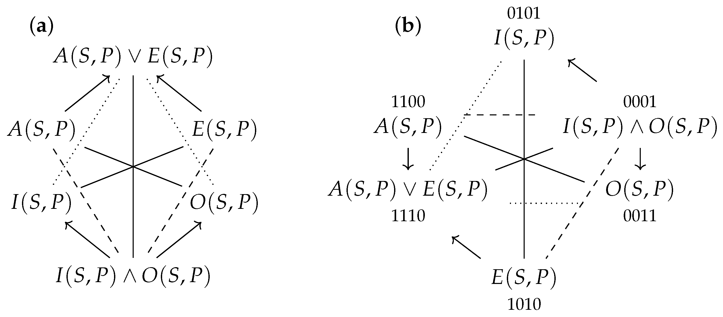
Finally, we turn to the second ‘heterogeneous’ case, which is the one that we will be studying for the remainder of this section. Suppose that we compute the Boolean closure of relative to , but then determine the Aristotelian relations relative to (i.e., and ). In comparison to the JSB hexagon for , the fact that has switched from to entails that some Aristotelian relations are lost, while others are maintained. For example, and are -contrary and are also -contrary; by contrast, and go from being -contrary to being -unconnected. In summary, we find that the Aristotelian diagram for is a U4 hexagon, which is shown twice in Figure 6. The depiction on the left should facilitate the comparison between the U4 hexagon for in Figure 6a and the JSB hexagon for in Figure 5a. By contrast, the depiction on the right is primarily meant to facilitate the comparison between the U4 hexagon for in Figure 6b and the U4 hexagon for in Figure 2b,c.
The latter comparison is formalized by the function that is defined below. It is easy to check that g is indeed an Aristotelian isomorphism from to . For example, we have that and are -contraries, while and , i.e., and , are -contraries. Finally, it bears emphasizing that even though as well as , it is not the case that is the identity map on . For example, g maps the formula onto a formula that is different from itself—even though belongs to , i.e., the codomain of g, and is thus ‘available’ as a potential g-image of . This quirk in the definition of g is the formal counterpart of the fact that we decided to draw the U4 hexagon for twice in Figure 6.
| ↦ | ||
| ↦ | ||
| ↦ | ||
| ↦ | ||
| ↦ | ||
| ↦ | ||
| ↦ |
We now turn to the bitstring semantics for . In order to compute the partition , we consider all conjunctions of (possibly negated) propositions from and discard those that turn out to be -inconsistent. This yields the following:
| = | { | |||||
| }. |
In general, one can show that for all logics (as in Definition 1) with a shared language and for all fragments , it holds that , i.e., the partition induced (in ) by the Boolean closure (in ) of the fragment is the same as the partition that is induced (still in ) by the fragment itself. In our specific case, we thus have that ; this is in line with earlier work, in which was already computed directly (without the ‘detour’ of first taking the Boolean closure of —be it in or , be it with or without keeping ⊤ and ⊥); cf. Section 4 of [42].
For ease of notation, we will write the bitstring semantics that corresponds to the partition simply as . Since , the U4 hexagon for has a Boolean complexity of 4, and its formulas can be represented by means of bitstrings of length 4. For example, since is -equivalent to , it can be represented as the bitstring 1100, i.e., . The bitstrings of all six formulas in the U4 hexagon are shown in Figure 6b.
Once again, it is also interesting to investigate how the aforementioned function g interacts with the partitions and . Applying g conjunct-wise to the anchor formula of yields , which is precisely the anchor formula . Continuing along these lines, we find that the result of conjunct-wise application of g to the anchor formula is -equivalent to precisely the anchor formula , for . If we now try to apply g conjunct-wise to the last anchor formula , we find , which is -inconsistent; in other words, does not have a counterpart in . Once again, this means that the -bitstrings for can be viewed as the result of systematically deleting the fifth bit position in the -bitstrings for ; compare Figure 2c and Figure 6b.
To make this formally precise, consider again the function , which deletes a bitstring’s fifth bit position, and define the function (again, note that this does not mean that g is a Boolean isomorphism, since itself is not a Boolean algebra isomorphism, just like is not a Boolean algebra isomorphism either). It is easy to see that . Consider, for example, the formula from , and note that . Again, all of this is captured by the commutative diagram in Figure 7: (i) since the upper rectangle commutes, it holds that , and (ii) since the lower rectangle commutes, it holds that , i.e., .
Just like before, it is easy to see that there does not exist a Boolean isomorphism between and , since the former has a Boolean complexity of 5, whereas the latter has a Boolean complexity of 4. However, there does exist a Boolean isomorphism h from to , which is defined below. (Since every Boolean isomorphism is an Aristotelian isomorphism as well [42], it follows that h is also an Aristotelian isomorphism from to .)
| ↦ | ||
| p | ↦ | |
| ↦ | ||
| q | ↦ | |
| ↦ | ||
| ↦ | ||
| ↦ |
To see that is a Boolean isomorphism, consider the function . Since the bitstring semantics and are Boolean algebra isomorphisms, and this notion is closed under taking inverses and composition, the function is a Boolean algebra isomorphism as well. Furthermore, it is easy to see that . Consider, for example, the formula , and note that . All of this is captured by means of the commutative diagram in Figure 8: (i) since the upper rectangle commutes, it holds that , and (ii) since the lower triangle commutes, it holds that , i.e., .
Finally, it bears emphasizing that h and interact exactly as expected with the maps f, g, , and that were defined before. In particular, it is easy to check that ; for example, we have and . Furthermore, since (cf. Figure 4) and (cf. Figure 7) and (cf. Figure 8) it follows that . This is all summarized by the commutative diagram in Figure 9: the left part of this diagram is Figure 4, the right part is Figure 8, and the part that is obtained by ignoring and in the middle is Figure 7.
5. Theoretical Analysis
In the previous sections, we have seen that the Aristotelian diagram for is a U4 hexagon of Boolean complexity 5, while the diagrams for and for are U4 hexagons of Boolean complexity 4. It is thus natural to ask whether there exist U4 hexagons with any other Boolean complexities. Theorem 1 states that this is not the case:
Theorem 1.
The Aristotelian family of U4 hexagons has exactly two Boolean subfamilies, one corresponding to Boolean complexity 5 and one corresponding to Boolean complexity 4.
The remainder of this section is dedicated to proving Theorem 1, as well as providing some further philosophical comments and explanations. The proof is based on theoretical insights from [41]. (These insights are also applied in Section 5 of [47], which served as a direct technical template for the current section).
The U4 hexagons studied in this paper thus far are all concerned with a specific logical system and its object language; for example, the U4 hexagon in Figure 3 concerns the system and the fragment of formulas . By contrast, we can also consider a generic description of a U4 hexagon, as shown in Figure 10. This description does not refer to any specific logical system or object language, but merely specifies a configuration of Aristotelian relations holding between certain ‘placeholder elements’. In particular, these placeholders are collected in the set . We see, for example, that the generic description in Figure 10 specifies and to be contrary to each other, while and are specified as being unconnected (i.e., not standing in any Aristotelian relation to each other). Once again, note that these are generic placeholders that do not come from any specific logical system; consequently, the Aristotelian relations that are specified as holding (or not holding) among them are not defined relative to a concrete logical system either.
We cannot simply compute the partition that is induced by , since Definition 3 explicitly refers to a specific logical system (viz., in its requirement that the anchor formulas be -consistent). However, given a generic description of an Aristotelian family , we can always ‘approximate’ the notion of -consistency without having to refer to any specific logical system . This approximative notion is called ‘-consistency’, and is used to compute the partition induced by the generic description of the Aristotelian family .
Definition 7
(-consistency and generic partition). Let be an Aristotelian family, and let be the set of placeholder elements that appear in the generic description of . A conjunction of these placeholders is said to be -consistent iff it does not contain two conjuncts that are specified as being contradictory or contrary by the generic description of . The generic partition induced by is defined as follows:
For example, starting from , we see that the conjunction of placeholders is U4-inconsistent, since its first and last conjuncts (i.e., and ) are specified as being contrary by the generic description in Figure 10. By contrast, the conjunction is U4-consistent, as it does not contain any two conjuncts that are specified as being contradictory or contrary by the generic description in Figure 10. Furthermore, since this generic description specifies that is contrary to and (and thus there are subalternations from and from to ), the conjunction can be simplified to . By systematically going through all such conjunctions of placeholder elements of , simplifying whenever possible, and discarding the U4-inconsistent conjunctions, we find the generic partition induced by :
| = | { | |||||
| }. |
We now consider the anchor formula in some more detail. Note that is U4-consistent, by the construction of . Furthermore, is also guaranteed to be -consistent, for any concrete logical system and any -consistent formulas to fill in the placeholders , respectively. For example, if we fill in the placeholders as resp. , we find that is -consistent; cf. the anchor formula from Section 2. For another example, if we fill in the placeholders as resp. , we find that is -consistent; cf. the anchor formula from Section 3. To see that this consistency is always guaranteed, suppose toward a reductio that there exist some logical system and some -consistent formulas such that filling in the placeholders as resp. renders -inconsistent. Since is a conjunction of only two placeholders (after simplification), this -inconsistency can already be expressed by means of a (binary) Aristotelian relation, viz., and are -contradictory or -contrary. But this violates the U4-consistency of .
To summarize: since is a conjunction of at most two placeholders (after simplification), its U4-consistency suffices to guarantee its -consistency (for any logical system ). Since , and also contain at most two placeholders (after simplification), exactly the same remarks apply to them as well.
This stands in sharp contrast with . Once again, is U4-consistent, by the construction of . However, since is a conjunction of more than two placeholders (after simplification), this U4-consistency no longer suffices to guarantee its -consistency for all concrete logical systems and -consistent formulas to fill in the placeholders , respectively. For example, if we fill in the placeholders as resp. , we find that is -consistent; cf. the anchor formula from Section 2. By contrast, if we fill in the placeholders as resp. , we find that is -inconsistent; cf. the absence of any anchor formula in Section 3. (We emphasize that this conjunction, , is still U4-consistent, as it does not contain any two conjuncts that are specified as being contradictory or contrary by the generic description of U4 hexagons in Figure 10.)
We can now summarize the entire analysis. The generic partition consists of five conjunctions, which are all -consistent, by the construction of . The formulas have at most two conjuncts (after simplification), and hence, they are guaranteed to be -consistent as well (for any logical system and -consistent formulas to fill in the placeholders). By contrast, the formula has more than two conjuncts (after simplification), and hence, it is not guaranteed to be -consistent (for any logical system and -consistent formulas to fill in the placeholders). More precisely: on the one hand, there are logical systems and fragments such that the Aristotelian diagram for is a U4 hexagon and such that is -consistent (and thus ); on the other hand, there are logical systems and fragments such that the Aristotelian diagram for is a U4 hexagon and such that is -inconsistent (and thus ).
Since this is an exhaustive case analysis, we conclude that the Aristotelian family of U4 hexagons has exactly two Boolean subfamilies: one corresponding to Boolean complexity 5 and one corresponding to Boolean complexity 4, as stated in Theorem 1. The U4 hexagon for , as studied in Section 2, belongs to the former Boolean subfamily, while the U4 hexagons for and for , as studied in Section 3 and Section 4, belong to the latter Boolean subfamily.
6. Conclusions
In this paper, we have investigated the Aristotelian family of unconnectedness-4 (U4) hexagons. We showed that this family has precisely two Boolean subfamilies, corresponding to Boolean complexities 5 and 4 (Section 5). Leading up to this result, we first studied the oldest known U4 hexagon, which is the conversion closure of the classical square for categorical statements, and showed that it has a Boolean complexity of 5 and is closely related to the so-called ‘Gergonne relations’ (Section 2). We then studied a simple U4 hexagon of Boolean complexity 4, in the context of classical propositional logic (Section 3). Finally, we studied another U4 hexagon of Boolean complexity 4, which can also be obtained as a (quite subtle) kind of closure of the classical square for categorical statements (Section 4).
From a local perspective, focusing on the square of opposition for the categorical statements, it is interesting to observe that two different kinds of closure operations yield two U4 hexagons, albeit of different Boolean complexities. From a more general, classificatory perspective, the results of this paper fit in nicely with the ongoing research efforts toward developing a comprehensive typology of Aristotelian families and their Boolean subfamilies. As we have seen throughout this paper, the family of U4 hexagons has interesting applications throughout philosophical logic, but it is also interesting in its own right. For example, one can define a -structure as a pair , with such that for all and for all . This defines another infinite sequence of Aristotelian families that can be fruitfully studied [48], and that has the family of U4 hexagons as its first non-trivial member. In particular, it is easy to check that -structures are simply pairs of contradictories (PCDs), -structures are classical squares of opposition, and -structures are U4 hexagons. (In recent, hitherto unpublished research, we found the first concrete application of a -structure.) It will be interesting to systematically investigate what the Boolean subfamilies are of the Aristotelian family of -structures, for each . The Boolean subfamilies of the families of PCDs () and of classical squares () were already known; this paper has investigated the Boolean subfamilies of the family of U4 hexagons (), thus allowing us to start exploring some regularities for increasing n. This will be taken up in further research.
Author Contributions
Both authors contributed equally to (all aspects of) this paper. All authors have read and agreed to the published version of the manuscript.
Funding
This research was funded by the research project ‘BITSHARE: Bitstring Semantics for Human and Artificial Reasoning’ (IDN-19-009, Internal Funds KU Leuven) and the ERC starting grant ‘STARTDIALOG: Towards a Systematic Theory of Aristotelian Diagrams in Logical Geometry’, funded by the European Union (ERC, STARTDIALOG, 101040049). The views and opinions expressed are those of the author(s) only and do not necessarily reflect those of the European Union or the European Research Council Executive Agency. Neither the European Union nor the granting authority can be held responsible for them. The first author holds a research professorship (BOFZAP) at KU Leuven.
![Axioms 13 00076 i001]()

Data Availability Statement
Data are contained within the article.
Acknowledgments
The authors would like to thank Alex De Klerck, Stef Frijters, Hans Smessaert and three anonymous reviewers for the interesting discussions and feedback on an earlier version of this paper.
Conflicts of Interest
The authors declare no conflicts of interest. The funders had no role in the design of the study; in the collection, analyses, or interpretation of data; in the writing of the manuscript, or in the decision to publish the results.
References
- Béziau, J.Y. New Light on the Square of Oppositions and its Nameless Corner. Log. Investig. 2003, 10, 218–232. [Google Scholar]
- Béziau, J.Y.; Jacquette, D. (Eds.) Around and Beyond the Square of Opposition; Springer: Basel, Switzerland, 2012. [Google Scholar]
- Béziau, J.Y.; Payette, G. (Eds.) The Square of Opposition. A General Framework for Cognition; Peter Lang: Bern, Switzerland, 2012. [Google Scholar]
- Béziau, J.Y.; Basti, G. (Eds.) The Square of Opposition: A Cornerstone of Thought; Springer: Cham, Switzerland, 2017. [Google Scholar]
- Béziau, J.Y.; Gerogiorgakis, S. (Eds.) New Dimensions of the Square of Opposition; Philosophia: Munich, Germany, 2017. [Google Scholar]
- Béziau, J.Y.; Vandoulakis, I.M. (Eds.) The Exoteric Square of Opposition; Springer: Cham, Switzerland, 2022. [Google Scholar]
- Parsons, T. The Traditional Square of Opposition. In Stanford Encyclopedia of Philosophy (Summer 2017 Edition); Zalta, E.N., Ed.; CSLI: Stanford, CA, USA, 2017. [Google Scholar]
- Jacoby, P. A Triangle of Opposites for Types of Propositions in Aristotelian Logic. New Scholast. 1950, 24, 32–56. [Google Scholar] [CrossRef]
- Sesmat, A. Logique II. Les Raisonnements. La Syllogistique; Hermann: Paris, France, 1951. [Google Scholar]
- Blanché, R. Sur l’opposition des concepts. Theoria 1953, 19, 89–130. [Google Scholar] [CrossRef]
- Blanché, R. Structures Intellectuelles. Essai sur L’organisation Systématique des Concepts; Librairie Philosophique J. Vrin: Paris, France, 1966. [Google Scholar]
- Czeżowski, T. On Certain Peculiarities of Singular Propositions. Mind 1955, 64, 392–395. [Google Scholar] [CrossRef]
- Kraszewski, Z. Logika stosunków zakresowych (Logic of extensional relations). Stud. Log. 1956, 4, 63–116. [Google Scholar] [CrossRef]
- Lilje, G.W. Singular Statements. Teach. Philos. 1987, 10, 219–225. [Google Scholar] [CrossRef]
- Moktefi, A.; Schang, F. Another Side of Categorical Propositions: The Keynes–Johnson Octagon of Oppositions. Hist. Philos. Log. 2023, 44, 459–475. [Google Scholar] [CrossRef]
- Kretzmann, N. William of Sherwood’s Introduction to Logic; University of Minnesota Press: Minneapolis, MN, USA, 1966. [Google Scholar]
- Khomskii, Y. William of Sherwood, Singular Propositions and the Hexagon of Opposition. In The Square of Opposition. A General Framework for Cognition; Béziau, J.Y., Payette, G., Eds.; Peter Lang: Bern, Switzerland, 2012; pp. 43–60. [Google Scholar]
- Maloney, T.S. Roger Bacon: The Art and Science of Logic; Pontifical Institute of Mediaeval Studies: Toronto, ON, Canada, 2009. [Google Scholar]
- Maloney, T.S. Lambert of Auxerre: Logica, or Summa Lamberti; University of Notre Dame Press: Notre Dame, IN, USA, 2015. [Google Scholar]
- Klima, G. John Buridan, Summulae de Dialectica; Yale University Press: New Haven, CT, USA, 2001. [Google Scholar]
- Read, S. John Buridan’s Theory of Consequence and His Octagons of Opposition. In Around and Beyond the Square of Opposition; Béziau, J.Y., Jacquette, D., Eds.; Springer: Berlin, Germany, 2012; pp. 93–110. [Google Scholar]
- Demey, L. Boolean Considerations on John Buridan’s Octagons of Opposition. Hist. Philos. Log. 2019, 40, 116–134. [Google Scholar] [CrossRef]
- Thiel, C. The Twisted Logical Square. In Calculemos… Matemáticas y libertad. Homenaje a Miguel Sánchez-Mazas; Echeverría, J., de Lorenzo, J., Peña, L., Eds.; Editorial Trotta: Madrid, Spain, 1996; pp. 119–126. [Google Scholar]
- Fogelin, R.J. Evidence and Meaning; Humanities Press: New York, NY, USA, 1967. [Google Scholar]
- Schumann, A. On Two Squares of Opposition: The Leśniewski’s Style Formalization of Synthetic Propositions. Acta Anal. 2013, 28, 71–93. [Google Scholar] [CrossRef]
- Massin, O. Pleasure and its Contraries. Rev. Philos. Psychol. 2014, 5, 15–40. [Google Scholar] [CrossRef]
- Horn, L.R. A Natural History of Negation; University of Chicago Press: Chicago, IL, USA, 1989. [Google Scholar]
- Horn, L.R. Histoire d’*O: Lexical Pragmatics and the Geometry of Opposition. In The Square of Opposition. A General Framework for Cognition; Béziau, J.Y., Payette, G., Eds.; Peter Lang: Bern, Switzerland, 2012; pp. 393–426. [Google Scholar]
- Ziegeler, D. On the Empty O-corner of the Aristotelian Square: A View from Singapore English. J. Pragmat. 2017, 115, 1–20. [Google Scholar] [CrossRef]
- Hruschka, J.; Joerden, J. Supererogation: Von deontologischen Sechseck zum deontologischen Zehneck. Arch. Philos. Law Soc. Philos. 1987, 73, 93–123. [Google Scholar]
- O’Reilly, D.T. Using the square of opposition to illustrate the deontic and alethic relations constituting rights. Univ. Tor. Law J. 1995, 45, 279–310. [Google Scholar] [CrossRef]
- de Oliveira Lima, J.A.; Griffo, C.; Almeida, J.P.A.; Guizzardi, G.; Aranha, M.I. Casting the Light of the Theory of Opposition onto Hohfeld’s Fundamental Legal Concepts. Leg. Theory 2021, 27, 2–35. [Google Scholar] [CrossRef]
- Ciucci, D.; Dubois, D.; Prade, H. Structures of Opposition in Fuzzy Rough Sets. Fundam. Inform. 2015, 142, 1–19. [Google Scholar] [CrossRef]
- Ciucci, D.; Dubois, D.; Prade, H. Structures of opposition induced by relations. The Boolean and the gradual cases. Ann. Math. Artif. Intell. 2016, 76, 351–373. [Google Scholar] [CrossRef]
- Schumann, A.; Wolenski, J. Two Squares of Oppositions and Their Applications in Pairwise Comparisons Analysis. Fundam. Inform. 2016, 144, 241–254. [Google Scholar] [CrossRef]
- Demey, L.; Smessaert, H. Geometric and Cognitive Differences between Aristotelian Diagrams for the Boolean Algebra B4. Ann. Math. Artif. Intell. 2018, 83, 185–208. [Google Scholar] [CrossRef]
- Vignero, L. Combining and Relating Aristotelian Diagrams. In Diagrammatic Representation and Inference; Basu, A., Stapleton, G., Linker, S., Legg, C., Manalo, E., Viana, P., Eds.; LNCS 12909; Springer: Cham, Switzerland, 2021; pp. 221–228. [Google Scholar]
- Frijters, S. Generalizing Aristotelian Relations and Diagrams. In Diagrammatic Representation and Inference; Giardino, V., Linker, S., Burns, R., Bellucci, F., Boucheix, J.M., Viana, P., Eds.; LNCS 13462; Springer: Cham, Switzerland, 2022; pp. 329–337. [Google Scholar]
- De Klerck, A.; Vignero, L.; Demey, L. Morphisms between Aristotelian Diagrams. Log. Univers. 2023. [Google Scholar] [CrossRef]
- Demey, L.; Frijters, S. Logic-Sensitivity and Bitstring Semantics in the Square of Opposition. J. Philos. Log. 2023, 52, 1703–1721. [Google Scholar] [CrossRef]
- Demey, L. Computing the Maximal Boolean Complexity of Families of Aristotelian Diagrams. J. Log. Comput. 2018, 28, 1323–1339. [Google Scholar] [CrossRef]
- Demey, L.; Smessaert, H. Combinatorial Bitstring Semantics for Arbitrary Logical Fragments. J. Philos. Log. 2018, 47, 325–363. [Google Scholar] [CrossRef]
- Frijters, S.; Demey, L. The Modal Logic of Aristotelian Diagrams. Axioms 2023, 12, 471. [Google Scholar] [CrossRef]
- Pellissier, R. Setting n-Opposition. Log. Univers. 2008, 2, 235–263. [Google Scholar] [CrossRef]
- Keynes, J.N. Studies and Exercises in Formal Logic, 3rd ed.; MacMillan: London, UK, 1894. [Google Scholar]
- Johnson, W. Logic. Part I; Cambridge University Press: Cambridge, UK, 1921. [Google Scholar]
- Demey, L.; Smessaert, H. Aristotelian and Boolean Properties of the Keynes-Johnson Octagon of Opposition. Log. Geom. 2023. Under review. [Google Scholar]
- Demey, L. From Euler Diagrams in Schopenhauer to Aristotelian Diagrams in Logical Geometry. In Language, Logic, and Mathematics in Schopenhauer; Lemanski, J., Ed.; Springer: Cham, Switzerland, 2020; pp. 181–205. [Google Scholar]
- Furs, S.N. Computation of Aristotle’s and Gergonne’s Syllogisms. Stud. Log. 1987, 46, 209–225. [Google Scholar] [CrossRef]
- Dekker, P. Not only Barbara. J. Logic, Lang. Inf. 2015, 24, 95–129. [Google Scholar] [CrossRef]
- Gergonne, J.D. Essai de Dialectique Rationelle. Ann. Math. Pures Appl. 1817, 7, 189–228. [Google Scholar]
- Giard, L. La “Dialectique Rationnelle” de Gergonne. Rev. D’Hist. Des Sci. 1972, 25, 97–124. [Google Scholar] [CrossRef]
- Faris, J.A. The Gergonne relations. J. Symb. Log. 1955, 20, 207–231. [Google Scholar] [CrossRef]
- Thomas, I. Eulerian Syllogistic. J. Symb. Log. 1957, 22, 15–16. [Google Scholar] [CrossRef]
- Thomas, I.; Orth, D. Axioms for the “Gergonne”-Relations. J. Symb. Log. 1959, 24, 305. [Google Scholar] [CrossRef]
- Thomas, I. Independence of Faris-Rejection-Axioms. Notre Dame J. Form. Log. 1960, 1, 48–51. [Google Scholar] [CrossRef]
- Smessaert, H.; Demey, L. Logical and Geometrical Complementarities between Aristotelian Diagrams. In Diagrammatic Representation and Inference; Dwyer, T., Purchase, H., Delaney, A., Eds.; LNCS 8578; Springer: Berlin, Germany, 2014; pp. 246–260. [Google Scholar]
- Demey, L.; Smessaert, H. The Interaction between Logic and Geometry in Aristotelian Diagrams. In Diagrammatic Representation and Inference; Jamnik, M., Uesaka, Y., Elzer Schwartz, S., Eds.; LNCS 9781; Springer: Berlin, Germany, 2016; pp. 67–82. [Google Scholar]
- García-Cruz, J.D.; Demey, L. Aristotelian Diagrams for the Ancient Discussion on Privative and Infinite Negation. Lorenz Demey 2023. Under review. [Google Scholar]
- Demey, L.; Smessaert, H. Metalogical Decorations of Logical Diagrams. Log. Univers. 2016, 10, 233–292. [Google Scholar] [CrossRef]
- Demey, L. Metalogic, Metalanguage and Logical Geometry. Log. Anal. 2019, 248, 453–478. [Google Scholar]
- Greniewski, H. Próba “Odmłodzenia” kwadratu logicznego (The square of opposition—A new approach). Stud. Log. 1953, 1, 276–297. [Google Scholar] [CrossRef]
- Rybaříková, Z. Prior on Aristotle’s Logical Squares. Synthese 2016, 193, 3473–3482. [Google Scholar] [CrossRef]
- Wybraniec-Skardowska, U. Logical Squares for Classical Logic Sentences. Log. Univers. 2016, 10, 293–312. [Google Scholar] [CrossRef]
- Luzeaux, D.; Sallantin, J.; Dartnell, C. Logical Extensions of Aristotle’s Square. Log. Univers. 2008, 2, 167–187. [Google Scholar] [CrossRef]
- Pizzi, C. Generalization and Composition of Modal Squares of Opposition. Log. Univers. 2016, 10, 313–325. [Google Scholar] [CrossRef]
- Pizzi, C. Contingency Logics and Modal Squares of Opposition. In New Dimensions of the Square of Opposition; Béziau, J.Y., Gerogiorgakis, S., Eds.; Philosophia Verlag: Munich, Germany, 2017; pp. 201–220. [Google Scholar]
- Jacoby, P. Contrariety and the Triangle of Opposites in Valid Inferences. New Scholast. 1960, 34, 141–169. [Google Scholar] [CrossRef]
- Béziau, J.Y. The Power of the Hexagon. Log. Univers. 2012, 6, 1–43. [Google Scholar] [CrossRef]
- Smessaert, H. The Classical Aristotelian Hexagon Versus the Modern Duality Hexagon. Log. Univers. 2012, 6, 171–199. [Google Scholar] [CrossRef]
- Moretti, A. Why the Logical Hexagon? Log. Univers. 2012, 6, 69–107. [Google Scholar] [CrossRef]
- Seuren, P. The Cognitive Ontogenesis of Predicate Logic. Notre Dame J. Form. Log. 2014, 55, 499–532. [Google Scholar] [CrossRef]
- Seuren, P.; Jaspers, D. Logico-cognitive structure in the lexicon. Language 2014, 90, 607–643. [Google Scholar] [CrossRef]
- Jaspers, D.; Seuren, P. The Square of Opposition in Catholic Hands. Log. Anal. 2016, 233, 1–35. [Google Scholar]
- Smessaert, H. On the 3D Visualisation of Logical Relations. Log. Univers. 2009, 3, 303–332. [Google Scholar] [CrossRef]
Figure 1.
Three Aristotelian diagrams for classical propositional logic (): (a) classical square of opposition (b) JSB hexagon (of Boolean complexity 3), (c) JSB hexagon (of Boolean complexity 4). The Aristotelian relations are visualized as usual: full, dashed, and dotted lines visualize resp. contradiction, contrariety, and subcontrariety, while arrows visualize subalternation.

Figure 2.
(a) Classical square of opposition for , (b) U4 hexagon for , (c) U4 hexagon for , together with the bitstring semantics .
Figure 2.
(a) Classical square of opposition for , (b) U4 hexagon for , (c) U4 hexagon for , together with the bitstring semantics .

Figure 3.
(a) U4 hexagon of opposition for , (b) U4 hexagon for , together with the bitstring semantics .
Figure 3.
(a) U4 hexagon of opposition for , (b) U4 hexagon for , together with the bitstring semantics .

Figure 4.
Commutative diagram for f, , , , and .

Figure 5.
(a) JSB hexagon for , (b) JSB hexagon for .

Figure 6.
(a) U4 hexagon for , (b) U4 hexagon for , drawn differently and together with the bitstring semantics .
Figure 6.
(a) U4 hexagon for , (b) U4 hexagon for , drawn differently and together with the bitstring semantics .

Figure 7.
Commutative diagram for g, , , and .

Figure 8.
Commutative diagram for h, , , and .

Figure 9.
Summarizing commutative diagram.

Figure 10.
Generic description of a U4 hexagon of opposition.


Table 1.
The formulas of and .
| (1.a) | (1) | ||
| (1.b) | |||
| (2.a) | (2) | ||
| (2.b) | |||
| (3.a) | (3) | ||
| (3.b) | |||
| (4.a) | (4) | ||
| (4.b) | |||
| (5.a) | (5) | ||
| (5.b) | |||
| (6.a) | (6) | ||
| (6.b) | |||
| (7.a) | ⊤ | ⊤ | (7) |
| (7.b) | |||
| (8.a) | ⊥ | ⊥ | (8) |
| (8.b) |
Disclaimer/Publisher’s Note: The statements, opinions and data contained in all publications are solely those of the individual author(s) and contributor(s) and not of MDPI and/or the editor(s). MDPI and/or the editor(s) disclaim responsibility for any injury to people or property resulting from any ideas, methods, instructions or products referred to in the content. |
© 2024 by the authors. Licensee MDPI, Basel, Switzerland. This article is an open access article distributed under the terms and conditions of the Creative Commons Attribution (CC BY) license (https://creativecommons.org/licenses/by/4.0/).
Share and Cite
MDPI and ACS Style
Demey, L.; Erbas, A. Boolean Subtypes of the U4 Hexagon of Opposition. Axioms 2024, 13, 76. https://doi.org/10.3390/axioms13020076
AMA Style
Demey L, Erbas A. Boolean Subtypes of the U4 Hexagon of Opposition. Axioms. 2024; 13(2):76. https://doi.org/10.3390/axioms13020076
Chicago/Turabian StyleDemey, Lorenz, and Atahan Erbas. 2024. "Boolean Subtypes of the U4 Hexagon of Opposition" Axioms 13, no. 2: 76. https://doi.org/10.3390/axioms13020076
Note that from the first issue of 2016, this journal uses article numbers instead of page numbers. See further details here.