Appendix A.1. Graphical Method
Here, we describe a simple rejection method, based on a graphical representation of mutations on a plane, that greatly reduces computation time when the final population size is very large.
Suppose we grow a bacterial population inside a flask, where diet and space requirements are fulfilled for up to
N cells and no cell dies. Taking
N as the carrying capacity and considering a constant per-generation growth rate
2 associated with each individual in the bacterial population, we have a pure-birth process where the reproduction of each member acts independently of the others, i.e., we have a stochastic process called the Yule process, a continuous-time homogeneous Markov chain [
39].
In this continuous-time setting, the population size reaches the carrying capacity N in generations and the population grows no further. Here, as in many biological contexts, time is measured in generations; i.e., is such that . Additionally, let us suppose is the mutation rate to mutator phenotypes and is the mutation rate of mutator cells to the marker phenotype.
With the above assumptions, the expected number of mutations to the mutator phenotype occurring from the beginning of the experiment until time
is
according to [
23] (Equation (
6)). Moreover, if
M is a random variable modeling the number of mutations occurring in the time interval
,
M follows a Poisson distribution by the law of small numbers theorem [
40] used as in [
23], so
The Yule process stochastically characterizes the lineage size of cells as individuals, e.g., see Equation (
A4). This notwithstanding, our framework leads to the following simplification: bacteria as a whole population grow deterministic as an exponential function; this is, given
, then
, with
, denotes the population size at time
t.
Let
be the function such that
Hence, denotes the population size at time t compared to the final population, as a fraction.
Let be a random vector, where and , then C represents a cell birthed at time T with a mutation or, equivalently, a mutant cell that appeared at time T and belongs to the fraction F of the final population. By considering a random sample of size M from C, and scattering them within , we obtain feasible and not feasible mutants, since, regarding f as a probability density function, all feasible mutations lie under the graph of f, and disregard them otherwise.
Figure A1 shows an example of the above-described method.
Figure A1.
Graphical model for selecting feasible mutations. mutations were generated as random points on . The parameter for the final population size was , for the wild-type mutation rate was , and for the final time was . The graph of (black curve) played a discriminant role since all points below the graph of f (red points) represent actual mutations, while the rest of the points (blue points) were disregarded.
Let
be the number of actual mutations from wild-type to mutator cells. Without loss of generality, let us suppose
is the mutant cell associated with the
mutation,
. Let us note that each mutant cell
, appearing at time
, has
units of time to give rise to its clonal linage, i.e., a subpopulation of size
. Now, in a Yule process, the clone population size that starts with
individuals, each one with growth rate
, has a negative binomial (
) distribution with parameters
j and
([
39] (pp. 377–378); [
41] (Equation 3.15); [
42]).
Therefore,
is a random variable such that
since
denotes the number of cells in the linage of cell
, excluding the initial cell
. This is due to the support of the negative binomial distribution we are computationally working with [
43] (func.
rnbinom),
. When the support of this distribution is
, as in ([
39] (pp. 377–378); [
41] (Equation 3.15); [
42]), Equation (
A4) should be rewritten as
Furthermore, in both cases, the total number of mutators in the population at time
is
To incorporate mutant cells with mutator phenotypes, let us suppose they appear as the result of mutations within the mutator cells’ subpopulation. Then, mutant cells with mutator phenotypes can appear only along the growth cycle of each mutant cell , .
Let be a fixed index. We know there are exactly mutator cells that have been raised by mutator cell , and if any mutant cell with a mutator phenotype, i.e., a mutator cell with a marker mutation, is appearing will be in the time interval . Setting as the carrying capacity, mutant cells with mutator phenotypes have units of time to appear, which happens with frequency .
Consequently, under a similar reasoning for Equation (
A2), we have that the number of mutations leading to mutant cells with mutator phenotypes is a random variable
such that
Let , with and , a random sample of size . Hence, each , is a random point on , representing a potential mutant cell with a mutator phenotype, i.e., a mutator cell with a marker mutation.
Analogous to Equation (
A3), function
defined by
with
, plays the discriminant role for the
mutant cells with mutator phenotypes, where, as before, all points except those below the graph of
were disregarded since they represent actual mutant cells with mutator phenotypes.
Let
be the number of actual mutant cells with mutator phenotypes that appeared along the growth cycle of mutator cell
. Without loss of generality, let us say
represent mutant cells with mutator phenotypes, then, for each
, the mutant cell with a mutator phenotype
has
units of time to give rise to its offspring of size
, which, according to Equation (
A4),
is a random variable such that
for every
.
By repeating this process for each
, we have that the total number of mutators in the population at time
is
Furthermore, we can study the distribution of the numbers of mutator cells and mutant cells with mutator phenotypes, as shown in
Figure A2.
For a pseudocode description of the graphical model, see Algorithm A1.
| Algorithm A1: Graphical model pseudocode |
![Axioms 13 00117 i001]() |
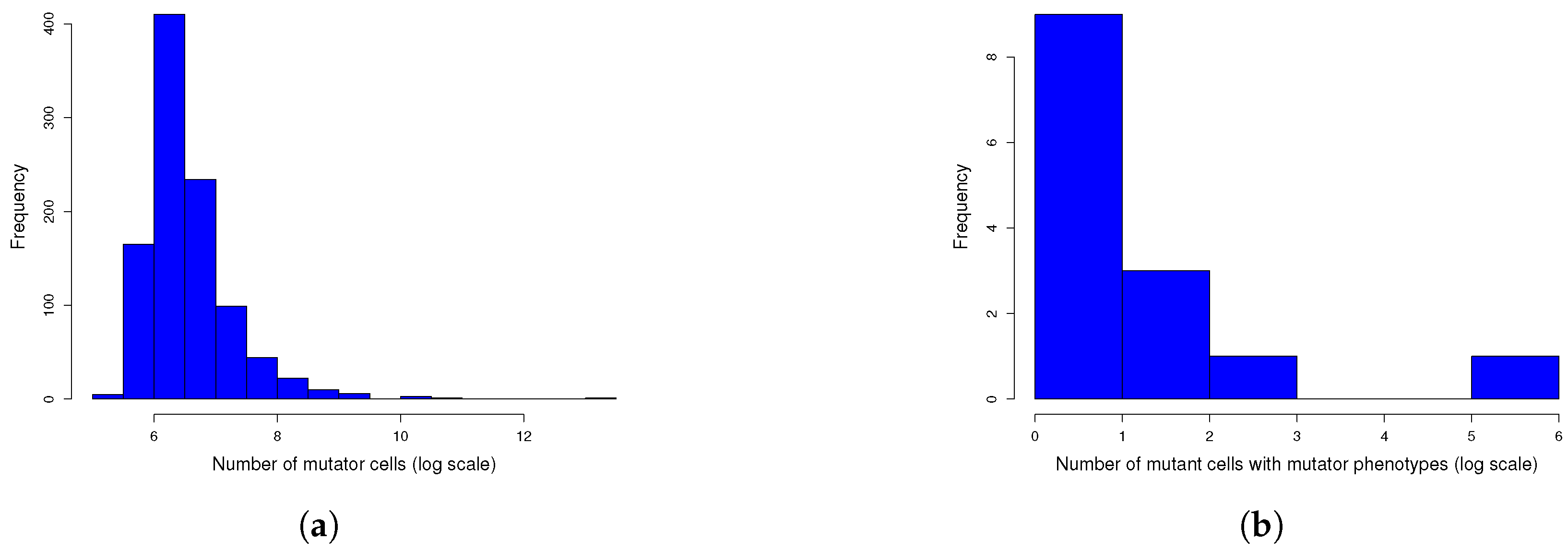
Figure A2.
One thousand simulations of graphical method. (
a) Histogram of the number of mutants on log scale and (
b) histogram of the number of mutators on log scale. Given the parameters in
Figure A1 and a mutation rate to mutator phenotype
, we simulated 1000 cultures in 354 s (printing plots) and in 5 s (printing no plots) of the described method. The distributions of the numbers of mutants and mutators were heavy-tailed, as expected.
Appendix A.2. Quantile Function Model
Let us recall that, given a function
, we say it is invertible if there exists a function
(called the inverse function of
g) such that
Definition A1 (Quantile function).
Let be a cumulative distribution function. The quantile function of F is defined by.
Quantile functions generalize the concept of the inverse of a function
g when
g is a cumulative distribution function. Now, quantile functions have a remarkable application, often called the inversion method, which is often employed to simulate random variables [
44] (Proposition 2), as will be used in the following method.
Under the assumptions and using the notation of the graphical model, given
,
denotes the population size at time
t. Then,
denotes the expected number of mutant cells at time
t, which, as a function, can be regarded as a probability density function. Furthermore, let
, then
, given by
is a probability density function, where its cumulative distribution function is
defined by
Hence, its quantile function is
given by
So, if
, then
is such that
, by the inversion method.
Applying the inversion method as above, only actual mutations leading to mutator phenotypes and their respective time of appearance are provided (see
Figure A3). Thus, instead of asking for the expected number of mutations, as in Equation (
A1), it is sufficient to ask for the expected number of mutators in the population, which is
Therefore, Equation (
A2) is rewritten as
Then, we can get the time of appearance of
M mutator cells by generating a random sample from
V of size
M,
. Note that, with this framework, there is no need to disregard any point. Therefore, the number of actual mutations
coincides with
M, which implies Equation (
A4) is rewritten as
and then, the total number of mutators in the population at time
is
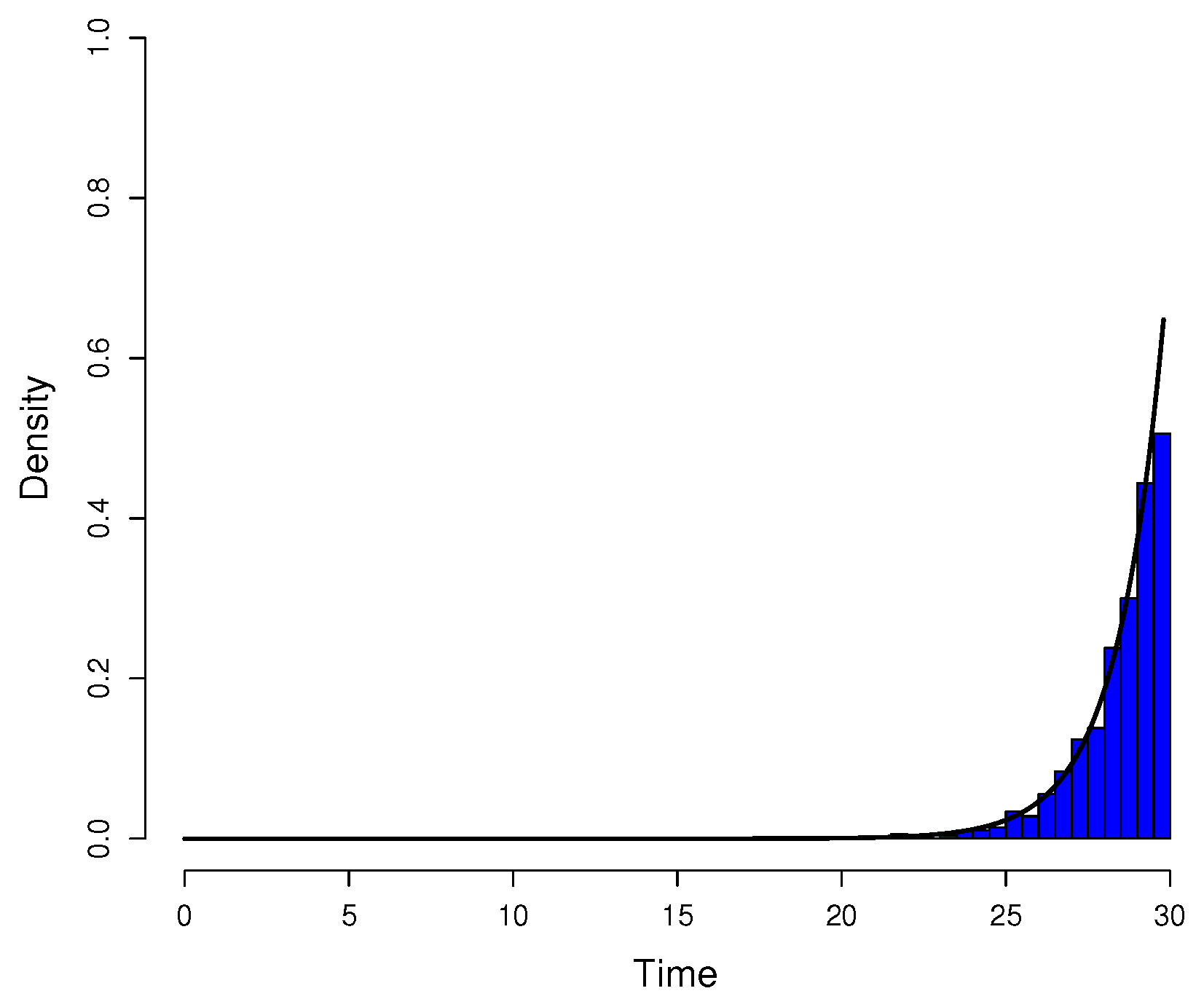
Figure A3.
Comparison between simulated data and actual probability density function. The parameters were the same as in
Figure A1. Data for the histogram of the time of appearance of mutant cells were simulated by the inversion method and Equation (
A14). The graph of
(black curve) was included for reference since the simulated data have distribution
h.
To incorporate mutant cells with mutator phenotypes, we proceed as in Equation (
A15). For each
, the expected number of mutants within the
mutator’s offspring of size
is
As a consequence, the random variable,
, counting the number of mutations leading to mutant cells with the
mutator phenotype, is such that
Now, given
, a fixed index, let
, then
, defined by
is the probability density function whose quantile function
is given by
Thus, if
, then
is such that
, where
.
Let
be a random sample from
, then
denotes the time of appearance of the
mutant cell with the
mutator phenotype. Therefore, analogous to Equation (
A17), the size of their offspring is a random variable
such that
This implies that the number of mutant cells with mutator phenotypes is
For a pseudocode description of the quantile function method, refer to Algorithm A2.
Figure A4.
(
a) Histogram of the number of mutants on log scale and (
b) histogram of the number of mutators on log scale. The same parameters of
Figure A2 were used to simulate 1000 cultures in two seconds using the quantile function method.
Figure A4.
(
a) Histogram of the number of mutants on log scale and (
b) histogram of the number of mutators on log scale. The same parameters of
Figure A2 were used to simulate 1000 cultures in two seconds using the quantile function method.

 ,
, 


