Article

Optimizing Controls to Track Moving Targets in an Intelligent Electro-Optical Detection System

College of Intelligence Science and Technology, National University of Defense Technology, Changsha 410073, China
*
Author to whom correspondence should be addressed.
Axioms 2024, 13(2), 113; https://doi.org/10.3390/axioms13020113
Submission received: 7 January 2024 / Revised: 28 January 2024 / Accepted: 3 February 2024 / Published: 8 February 2024
(This article belongs to the Special Issue Control Theory and Control Systems: Algorithms and Methods)

Abstract

:
Electro-optical detection systems face numerous challenges due to the complexity and difficulty of targeting controls for “low, slow and tiny” moving targets. In this paper, we present an optimal model of an advanced n-step adaptive Kalman filter and gyroscope short-term integration weighting fusion (nKF-Gyro) method with targeting control. A method is put forward to improve the model by adding a spherical coordinate system to design an adaptive Kalman filter to estimate target movements. The targeting error formation is analyzed in detail to reveal the relationship between tracking controller feedback and line-of-sight position correction. Based on the establishment of a targeting control coordinate system for tracking moving targets, a dual closed-loop composite optimization control model is proposed. The outer loop is used for estimating the motion parameters and predicting the future encounter point, while the inner loop is used for compensating the targeting error of various elements in the firing trajectory. Finally, the modeling method is substituted into the disturbance simulation verification, which can monitor and compensate for the targeting error of moving targets in real time. The results show that in the optimal model incorporating the nKF-Gyro method with targeting control, the error suppression was increased by up to 36.8% compared to that of traditional KF method and was 25% better than that of the traditional nKF method.

1. Introduction

Aerial threats have become an important aspect of defense technology and will present major challenges to security and counter-terrorism over the course of the next few years [1,2,3]. The aerial threat facing urban security is so-called “low, slow and tiny” unmanned drones that cannot easily be detected by radar [4,5]. In this case, unmanned light weapon stations (ULWSs) are the last line of defense. However, it is difficult to adapt the traditional optical sighting of general-purpose ULWSs to this latest security concern [6]. Electro-optical detection systems (EODSs), which are intelligent precision targeting devices with specific functions of target imaging and tracking [7,8,9,10,11,12], are playing an important role in tracking moving targets.
Liu X.Y. et al. [13] proposed a firing control method using an anti-aircraft gun based on a variable-step Runge–Kutta model. Zhang X.J. et al. [14] proposed a differential targeting model using a high-pressure water jet based on Newton’s second law. In order to improve the efficiency of firing data for shipboard guns, Yao Z. et al. [15] proposed a new targeting control model based on a gravitational search algorithm and secant method. Liu H. et al. [16] proposed a mathematical targeting model and mechanism that is imbedded in the rifle grip to counter the disturbance to line-of-sight and low action speed caused by manual firing. In order to improve targeting accuracy by controlling firing time, Geng Q. et al. [17] proposed a filter weighted fusion algorithm and linear predicting firing criterion. According to the characteristics of the controllable muzzle velocity of the new shipboard guns, Wu W. et al. [18] proposed a maximum targeting probability equation based on the dichotomy model and golden section. However, these methods based on the assumption of stationary targets produce unacceptably high errors when tracking moving targets such as “low, slow and tiny” unmanned drones.
Zhang Z.Y. et al. [19] proposed a firing model using an electromagnetic railgun against aerial targets within a line-of-sight range based on a 6-DOF exterior ballistic equation and a targeting probability model for single-shot and whole-route continuous-shot firing. Qiu X.B. et al. [20] used the current statistical model as an example to combine a moving target with pseudo-acceleration in polar coordinate systems using a Kalman filtering algorithm in the design. This solved the problem of targeting and firing control for tanks facing moving targets. Based on the exterior ballistics equation, Liu R. et al. [21] proposed a dynamic gunnery problem solution model. The angle and flight time of projectile are calculated iteratively synchronously, so as to improve the efficiency of the targeting control. Lyu M.M. et al. [22,23,24,25] proposed a series of miss-distance time-delay control methods for remotely operated weapon station platforms. The tests showed that the overshoot decreased to 2.5%. However, these models for tracking moving targets are only suitable for applications such as in artillery, tanks and missiles with long distances, high firing rates and large damage areas. In contrast, an EODS needs to control the targeting error within 10 pixels (about <1 mrad) in a lens of 1280 × 720 pixels to achieve precision shooting against “low, slow and tiny” unmanned drones. This highlights the higher accuracy requirements for predicting and targeting control methods in EODSs.
Moreover, a light weapon station equipped with an EODS needs to quickly track and aim at unmanned drone moving targets to achieve high-precision targeting control. There are still only a few types of targeting control methods for “low, slow and tiny (LST)” moving targets in EODS firing, and an adaptive filtering prediction model with high tracking precision is still in the exploratory stage.
In this paper, we present an optimal model of an advanced n-step adaptive Kalman filter and gyroscope short-term integration weighting fusion (nKF-Gyro) method with targeting control. A method is put forward to improve the model by adding a spherical coordinate system to design an adaptive Kalman filter and using a mathematical model to track moving targets. The targeting error formation is analyzed in detail to reveal the relationship between tracking controller feedback and line-of-sight position correction. Based on the establishment of a targeting control coordinate system for tracking moving targets, a dual closed-loop composite optimization control model is proposed. The outer loop is used for estimating the motion parameters and predicting the future encounter point, while the inner loop is used for compensating the targeting error of various elements in the firing trajectory. Finally, simulation experiments prove the effectiveness of the optimized model, which can monitor and compensate for the targeting error of moving targets in real time. The results show that the error suppression of the nKF-Gyro optimal method increased by up to 36.8% compared to that of the traditional KF method and was 25% better than that of the traditional nKF method.
This manuscript is valuable for all researchers who are interested in electro-optical detection systems, targeting controls, adaptive filters and moving targets.

2. Coordinate System for Targeting

Launching the bullet to the center of the target area is what an EODS aims to do. However, due to systematic errors and the factors that are simplified and ignored during modeling, the bullet always deviates from the target center. We define this deviation as the bullet–target error E(k) and Ω(k) as the target area.
E T ( k ) = {   0   E ( k ) Ω ( k ) E ( k ) E ( k ) Ω ( k )
In Equation (1), E T ( k ) is the miss-distance. As shown in Figure 1, the target center M q is the origin and the bullet–target encounter time t f . Point O represents the position where the EODS begins to target. The velocity of the bullet flying to point M q is V s ( t f ) . The velocity of the target moving to point M q is V m ( t f ) . Then, the parameter V re ( t f ) can be represented by the following equation.
V re ( t f ) = V s ( t f ) V m ( t f )
In Figure 1, we set point N in the coordinate system M q X Y Z as the actual targeting point. Then, the relationship of targeting error E can be obtained.
E = O N = ( X E , Z E ) T
In Equation (3), X E is the bullet–target error in the azimuth direction, Z E is the bullet–target error in the pitch direction. We set the targeting data when the bullet hits the target M q as ( α q , β q ) , and the targeting data correspond to the point N ( α N , β N ) . Then, the relationship of targeting error is Θ , where
Θ = [ Δ α q Δ β q ] = [ α q β q ] [ α N β N ]
In Equation (4), Δ α q and Δ β q are the azimuth and pitch errors of the targeting data in point M q . As shown in Figure 1b, O p M p approximates the vertical axis direction M q Y in the coordinate system M q X Y Z .
{ X E = D q tan Δ α E   Z E = D q tan Δ β E
Then, the relationship between the ( Δ α E , Δ β E ) and Θ can be obtained.
{ Δ α E Δ α q Δ β E Δ β q
Therefore, the targeting error Θ can be obtained by reducing the bullet–target error E.
As shown in Figure 2, we take O X Y Z as the geography coordinate system and O p X p Y p Z p is the EODS targeting coordinate system. K 1 K 2 is the target trajectory; k 1 k 2 is the projection of the target trajectory on the horizontal plane.
(1) At the moment of firing, the EODS moves to the point O p ( x p , y p , 0 ) . V p ( v p x , v p y , v p z ) is the movement speed of EODS; c p is the movement direction.
(2) At the moment of firing, the Cartesian coordinate of the target in system O X Y Z is the current encounter point M ( x m , y m , z m ) ; the spherical coordinate of the target in system O p X p Y p Z p is M ( D , α , β ) . d and h are the horizontal and vertical distance. α and β are the azimuth and pitch angle. V m ( v mx , v my , v mz ) is the movement speed of the target. The movement direction is consistent with the target trajectory K 1 K 2 .
(3) Suppose that the future encounter point is M q : the Cartesian coordinate of the point M q in system O X Y Z is M q ( x q , y q , z q ) ; the spherical coordinate of the point M q in system O p X p Y p Z p is M q ( D q , α q , β q ) . d q and h q are the horizontal and vertical distance. α q and β q are the azimuth and pitch angle. V q ( v q x , v q y , v q z ) is the movement speed of the target. The movement direction is consistent with the target trajectory K 1 K 2 .
(4) The O Y axis intercept of the target trajectory projection in system O X Y Z is y dd . V w ( v wx , v wy , v wz ) is the movement speed of the wind. c w is the movement direction.
Figure 3a shows how we predict the future encounter point M q through the moving target motion of the current encounter point M. Then, we solve the targeting data ( α , β ) of the future encounter point M q . ( α q ( t ) , β q ( t ) ) is the targeting data of the forward solution.
In Figure 3b, we use a certain moment in the moving target motion as the future encounter point M q to solve the targeting data ( α , β ) of the current encounter point M, which is called the inverse solution targeting equation. ( α q ( t t f ) , β q ( t t f ) ) are the targeting data of the inverse solution.
By analyzing the source of targeting error through forward solutions, the following quantitative relationship can be obtained.
E r r o r A = [ α N β N ] [ α q β q ]
In Equation (7), ( α N , β N ) are the actual targeting data in point N. ( α q , β q ) is the forward solution targeting error. E r r o r A is the error generated during the forward solution process.
By analyzing the source of targeting error through inverse solutions, the following quantitative relationship can be obtained.
[ α q β q ] = [ α q β q ] + E r r o r B
In Equation (8), ( α q , β q ) are the actual targeting data in point M q . ( α q , β q ) is the inverse solution targeting error. E r r o r B is the error generated during the inverse solution process. Combining Equations (4), (7) and (8), it can be concluded that,
Θ = [ α q β q ] [ α N β N ] = [ α q β q ] [ α q β q ] + E r r o r B E r r o r A
Simplify the Equation (9) with E r r o r A = E r r o r B = 0 ,
Θ = [ Δ α q Δ β q ] = [ α q β q ] [ α q β q ]
Therefore, the targeting error Θ can be seen as the difference between the inverse solution data ( α q , β q ) and the forward solution data ( α q , β q ) .

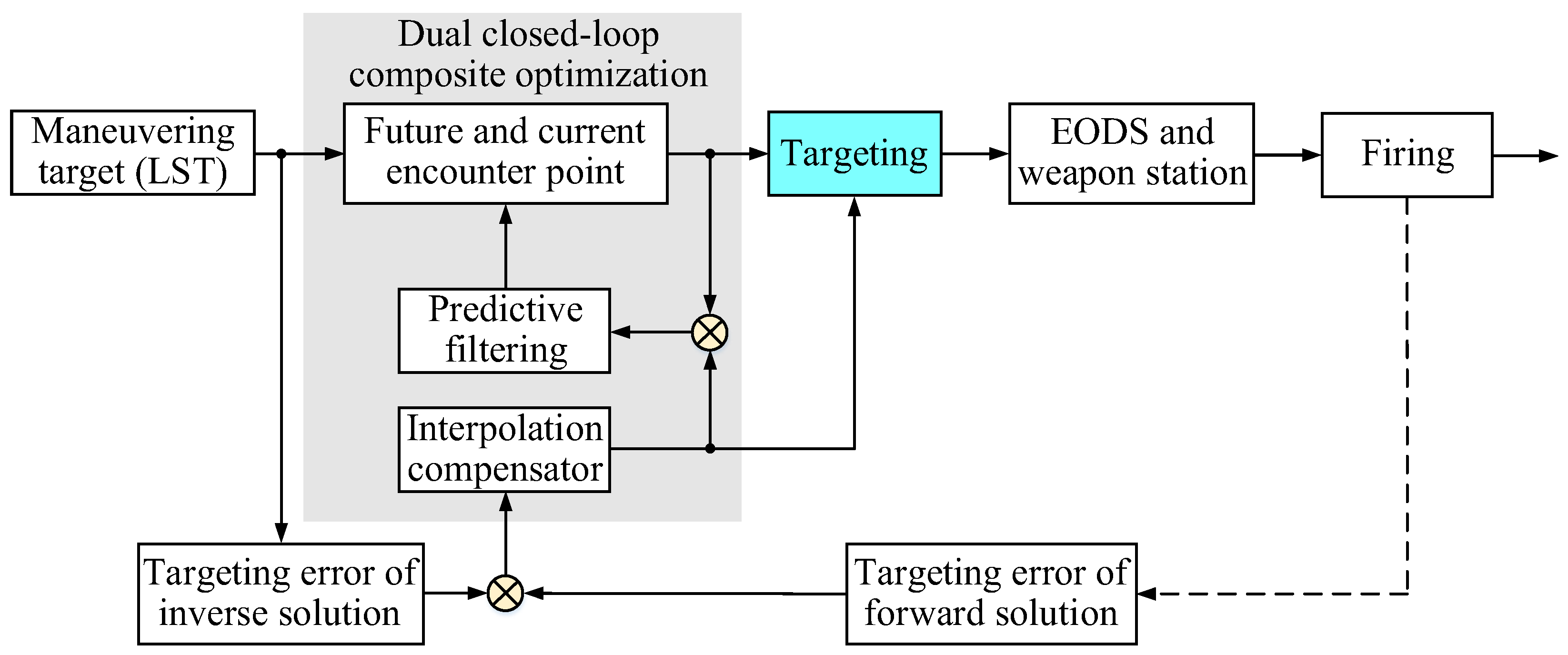
3. Design of Targeting Control

As shown in Figure 4, the outer loop is used for estimating the motion parameters and predicting the future encounter point, while the inner loop is used for compensating the targeting error of various elements in the firing trajectory. Targeting control is the core of the dual closed loop.

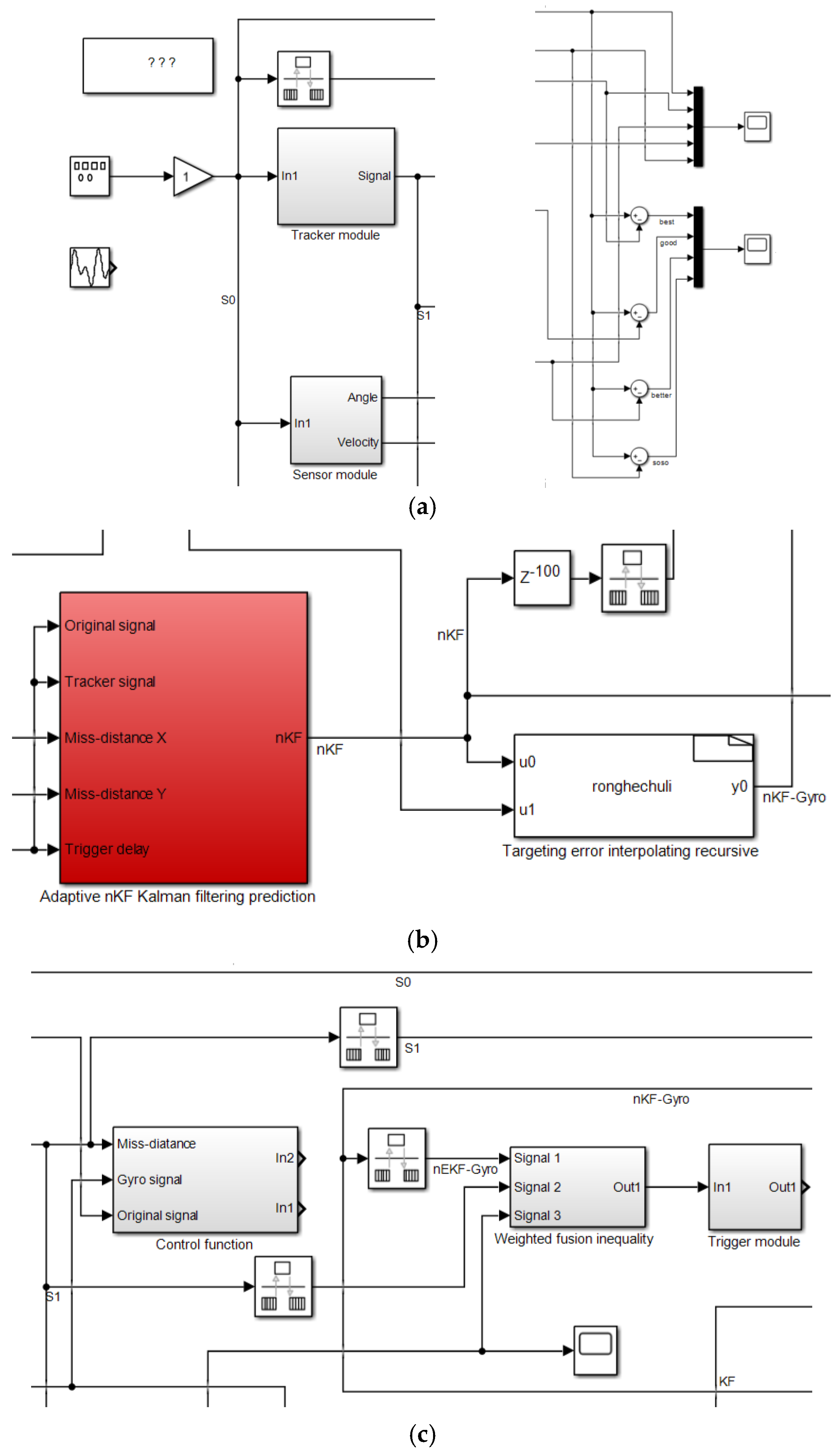
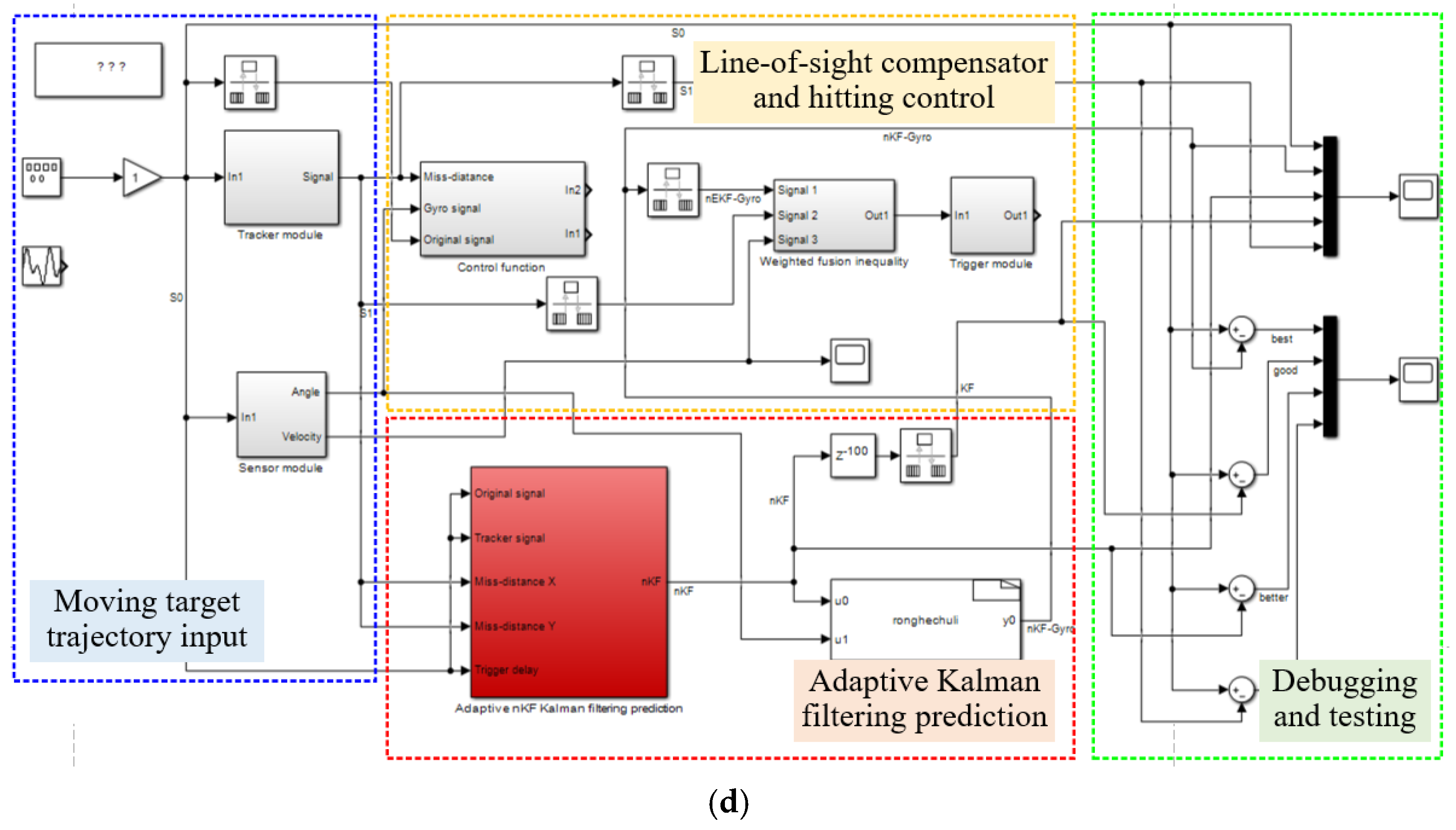
3.1. Adaptive nKF Kalman Filtering Prediction

We designed an adaptive angular rate prediction algorithm in the spherical coordinate system of the LST moving target constructed in Figure 2 for targeting control.
Treating the random disturbance received by the target in motion as system noise, as shown in Figure 5, we established a moving target motion model with an adaptive Kalman filtering equation. The expression of the target state vector was then obtained.
X s ( k ) = [ α ,   β ,   α ˙ ,   β ˙ ,   α ¨ ,   β ¨ ] T
In Equation (11), ( α , β ) are the azimuth and pitch angle of the moving target. ( α ˙ , β ˙ ) is the angular rate. ( α ¨ , β ¨ ) is the angular acceleration rate. X ^ s ( k + 1 | k ) is the target state vector at time k T and X s ( k ) is estimated at time ( k + 1 ) T .
Then, the expression Y ^ s ( k + 1 | k ) of the target angular state vector estimated at time ( k + 1 ) T can be obtained.
Y ^ s ( k + 1 | k ) = g s ( X ^ s ( k + 1 | k ) ) = ( α ˙ ^ ( k + 1 | k ) ,   β ˙ ^ ( k + 1 | k ) ) T
In Equation (12), ( α ˙ ^ ( k + 1 | k ) ,   β ˙ ^ ( k + 1 | k ) ) T is the vector expression for the estimated targeting error of the moving target at time ( k + 1 ) T . g s ( x ) is the kinematic function of the target. Then, the angular rate discrete time state equation of spherical coordinate is,
Z s ( k ) = H s ( k ) X s ( k ) + V s ( k )
In Equation (13), the observation matrix is,
H s ( k ) = [ 0 0 1 0 0 0 0 0 0 1 0 0 ]
The measurement noise is,
V s ( k ) = [ η 1 k η 2 k ]
In Equation (15), suppose that η 1 k and η 2 k are not correlated: then, the variance matrix of V s ( k ) is,
R s ( k ) = [ λ 1 k 2 0 0 λ 2 k 2 ]
Combining Equations (11)–(16), the KF standard Kalman filtering equation group is,
{ X ( k ) = Φ ( k + 1 | k ) X ( k ) + Γ ( k + 1 | k ) W ( k ) Z ( k ) = H ( k ) X ( k ) + V ( k )
Then, the quantitative relationship equation in spherical coordinates can be obtained. The one-step predictive filtering equation is,
X ^ s ( k + 1 | k ) = Φ ( k + 1 | k ) X ^ s ( k )
The one-step prediction mean square error estimation equation is,
P ( k + 1 | k ) = Φ ( k + 1 | k ) P ( k ) Φ T ( k + 1 | k ) + Q ( k )
The gain matrix equation is,
K ( k + 1 ) = P ( k + 1 | k ) H s T ( k + 1 ) ( H s ( k + 1 ) P ( k + 1 | k ) H s T ( k + 1 ) + R s ( k + 1 ) ) 1
The predictive estimation equation is,
X ^ s ( k + 1 ) = X ^ s ( k + 1 | k ) + K ( k + 1 ) ( Z ( k + 1 ) H s ( k + 1 ) X ^ s ( k + 1 | k ) )
Update the mean square error equation to,
P ( k + 1 ) = ( I K ( k + 1 ) H s ( k + 1 ) ) P ( k + 1 | k )
The one-step angular rate optimal prediction equation is,
Y ^ s ( k + 1 | k ) = g s ( X ^ s ( k + 1 | k ) )
In Equations (17)–(23), X s ( t ) is the n dimension state vector at time k. Φ ( k + 1 | k ) is the n × n dimension state transition matrix. Γ ( k + 1 | k ) is the n × p dimension noise input matrix. W ( k + 1 ) is a p dimension state noise sequence. Z s ( k + 1 ) is an m dimension observation sequence. H s ( k + 1 ) is the m × n dimension observation matrix. V ( k + 1 ) is the m dimension observation noise sequence, assuming the flight time of bullet is t f .
{ X ( k f + 1 | k f ) = Φ f X ^ ( k f | k f ) P ( k f + 1 | k f ) = Φ f P ( k f | k f ) Φ f T + Q
Then, the filtering equation group is,
{ X ^ ( k f | k f ) = X ^ ( k ) P ^ ( k f | k f ) = P ^ ( k )
Combining Equations (17)–(24) and (25), the adaptive filtering equation can be obtained.
Y ^ s ( k + f | k ) = g s ( X ^ s ( k + f | k ) ) = ( α ˙ ^ ( k + f | k ) ,   β ˙ ^ ( k + f | k ) ) T
In Equation (26), Y ^ s ( k + f | k ) is the optimal predicted value of f-step angular rate in the spherical coordinate system for targeting control.

3.2. Weighted Fusion Inequality Model

Assume that the number of signals detected by n sensors during a certain measurement stage is X = [ x 1 ,   x 2 ,   ,   x n ] T . Elements x 1 ,   x 2 ,   ,   x n are independent of each other in vector formulas. Set the variance of each element as σ 21 , σ 22 , , σ 2 n , respectively. Set the true value to be predicted as parameter x. Introduce the weighted factor vector W = [ w 1 ,   w 2 ,   ,   w n ] T into the equation.
i = 1 n w i = 1
Then, the weighted factor and the fused estimated value x ¯ equation can be obtained.
x ¯ = i = 1 n w i x i = W T X
In Equation (28), x ¯ is an unbiased estimate of x . Then, the total mean square error σ equation can be obtained.
σ 2 = E [ ( x x ¯ ) 2 ] = E [ i = 1 n w i 2 ( x x i ) 2 + 2 i = 1 , j = 1 i j n w i w j ( x x i ) ( x x j ) ]
The core of weighted fusion minimizes the signal variance by determining a set of weighting factors w i . In Figure 6, we assume that at time j , signal measurement data   x 1 ( j ) ,   x 2 ( j ) ,   ,   x i ( j ) are detected through n sensors. x i ( j ) = d i ( j ) + b i ( j ) is the signal detection value at time j. i refers to the i-th signal. d i ( j ) is the true value of the signal, b i ( j ) is the white noise of the i-th signal at time j, and the mean square deviation is σ i 2 . Then, the weighted fusion quantitative relationship of the n-th signal can be obtained.
s ( j ) = i = 1 n w i x i ( j ) = W T X ( j )
In Equation (30), X ( j ) = [ x 1 ( j ) ,   ,   x n ( j ) ] T are the sensor measurement data at time j. W = [ w 1 ,   ,   w n ] T is the unknown weight matrix to be estimated.
If i = 1 n w i = 1 , the unbiased estimation can be obtained. Due to   x 1 ( j ) ,   x 2 ( j ) ,   ,   x n ( j ) are independent of each other, and are an unbiased estimate of the true value x, so the equation E [ ( x x p ) ( x x q ) ] = 0 , ( p q ;   p = 1 ,   2 ,   ,   n ;   q = 1 ,   2 ,   ,   n ) can be obtained.
σ 2 = E [ i = 1 n w i 2 ( x x i ) 2 ] = i = 1 n w i 2 σ i 2
Using the Cauchy–Schwarz inequality and the weighted fusion function definition of Equations (28), (29) and (31), the mathematical model can be obtained.
( i = 1 n w i 2 σ i 2 ) ( i = 1 n 1 σ i 2 ) ( i = 1 n w i 2 ) 2 = 1
In Equation (32), the corresponding minimum mean square error equation is,
σ min 2 = V [ s ( j ) ] = E [ s ( j ) E [ s ( j ) 2 ] ] = 1 / i = 1 n 1 σ i 2

3.3. Targeting Error Interpolating Recursive
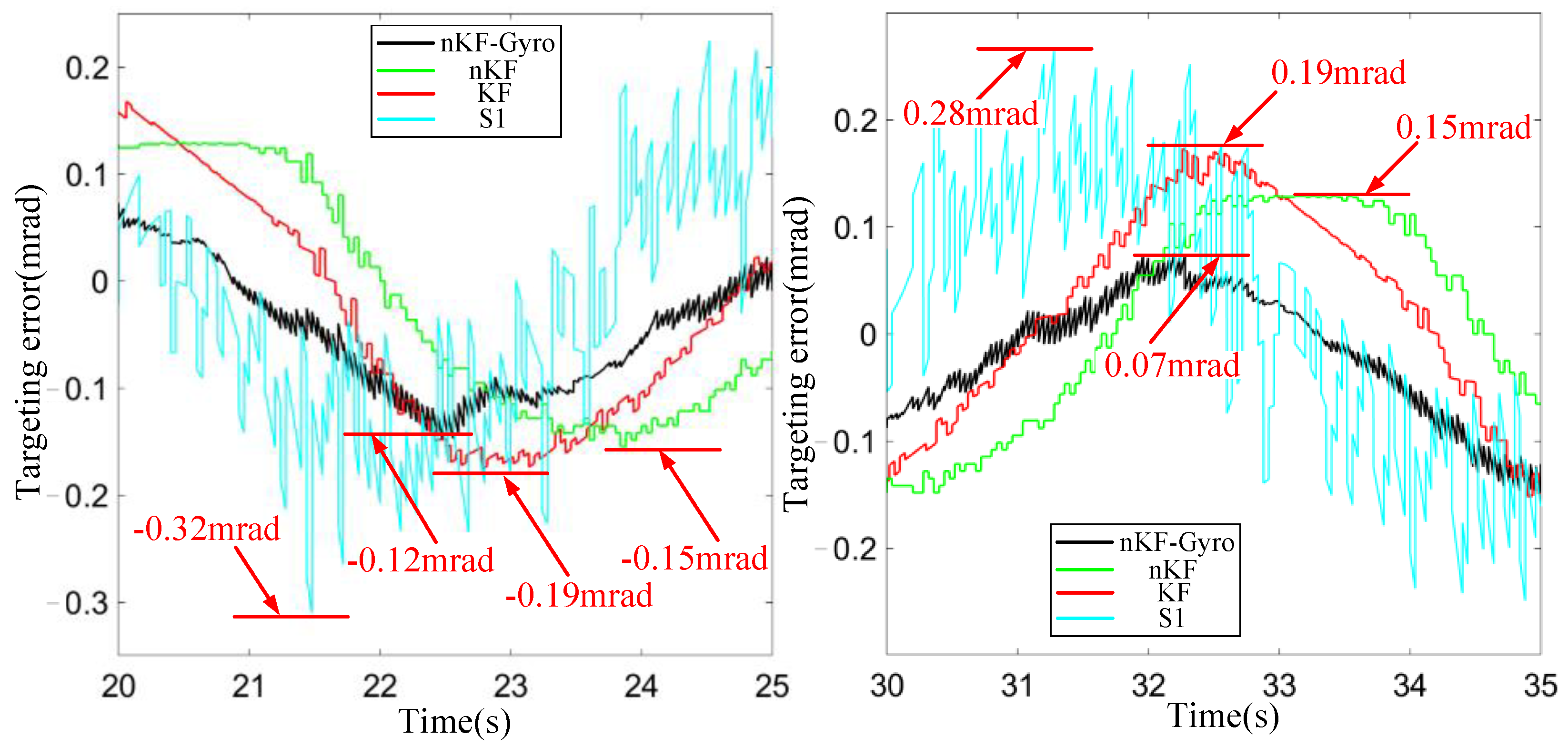
Substitute the position estimation ( x 0 ,   y 0 , z 0 ) = ( x ^ ( k ) ,   y ^ ( k ) , z ^ ( k ) ) and velocity estimation ( v x ,   v y ,   v z ) = ( v ^ x ( k ) ,   v ^ y ( k ) ,   v ^ z ( k ) ) into the following targeting equation group,
{ x = x 0 + v x t y = y 0 + v y t z = z 0 + v z t D = D ( t ) = x 2 + y 2 + z 2
Equation (35) is,
t = g ( D ,   h ) = t f ( d ,   h )
Combining Equations (9) and (10), the targeting data equation for point M q is,
{ α q = α ( x , y , z ) + Δ α ( x , y , z ) β q = β ( x , y , z ) + Δ β ( x , y , z )
Substitute the estimated position ( x ^ ( k ) ,   y ^ ( k ) , z ^ ( k ) ) into Equation (36). Then, substitute it into Equations (34) and (35) to solve the equation of the bullet flight time,
t = t f ( d ,   h ) = t f [ x ^ 2 ( k ) + y ^ 2 ( k ) ,   h ^ ( k ) ]
Add the targeting data equation,
{ α q = α ( x ^ ( k ) ,   y ^ ( k ) , z ^ ( k ) ) + Δ α ( x ^ ( k ) ,   y ^ ( k ) , z ^ ( k ) ) β q = β ( x ^ ( k ) ,   y ^ ( k ) , z ^ ( k ) ) + Δ β ( x ^ ( k ) ,   y ^ ( k ) , z ^ ( k ) )
If ( k Δ T t f ( k ) ) 0 , take m = k Δ T t f ( k ) Δ T , and k Δ T t f ( k ) is exactly an integer multiple of Δ T . The following equation can then be derived.
k Δ T t f ( k ) = int ( k Δ T t f ( k ) Δ T )
The targeting data of inverse solution at time t k m are,
{ α q ( k m ) = α q [ t k t f ( k ) ] β q ( k m ) = β q [ t k t f ( k ) ]
If k Δ T t f ( k ) is not an integer multiple of Δ T , it is necessary to calculate the targeting data of inverse solution at time t k 1 , and then obtain the targeting data at time t k m through interpolation recursive compensation.
{ α q ( k m ) = ( k m ) Δ T t f ( k ) Δ T + t f ( k 1 ) t f ( k ) α q [ ( k 1 ) Δ T t f ( k 1 ) ] ( k m 1 ) Δ T t f ( k 1 ) Δ T + t f ( k 1 ) t f ( k ) α q [ k Δ T t f ( k ) ] β q ( k m ) = ( k m ) Δ T t f ( k ) Δ T + t f ( k 1 ) t f ( k ) β q [ ( k 1 ) Δ T t f ( k 1 ) ] ( k m 1 ) Δ T t f ( k 1 ) Δ T + t f ( k 1 ) t f ( k ) β q [ k Δ T t f ( k ) ]
Similarly, as shown in Figure 7, Equation (41) can also be used to obtain the interpolation recursive equation group for targeting data of forward solutions.

4. Verification

To verify the effectiveness of the adaptive line-of-sight (LOS) filtering and targeting control model, the Matlab/Simulink algorithm (nKF-Gyro) shown in Figure 8 was built to validate and compare data. Part 1 is the moving target trajectory input and debugging testing. Part 2 is the adaptive Kalman filtering prediction. Part 3 is the line-of-sight compensator and targeting control.
Figure 9 shows a snake-shaped flight trajectory curve of a moving target, assuming that the target is moving in a constant acceleration (CA) motion. We assume that the X-axis trajectory of the target satisfies sine equation x = A sin ( ω 1 a + φ 1 ) + b , and the Y-axis trajectory of the target satisfies cosine equation y = B cos ( ω 2 a + φ 2 ) + b . The target is moving in space 0→80 m on the Z-axis. Parameters A ,   B ,   a ,   b and ω 1 ,   ω 2 ,   φ 1 ,   φ 2 are both constant values. Taking the targeting data in the azimuth X-direction as an example, the typical test curve is shown in Figure 10, Figure 11, Figure 12 and Figure 13.
Figure 10 and Figure 12 are the comparison of targeting data. The black curve S0 represents the targeting true value. The red curve S1 represents the actual measured value. The dark blue curve represents the measured value of the traditional KF method. The green curve represents the measured value of the traditional nKF method. The light blue curve represents the measured value of the optimized nKF-Gyro method.
Similarly, Figure 11 and Figure 13 show the comparison of targeting errors for the corresponding methods KF, nKF, nKF-Gyro, and S3 measured value. Figure 12 and Figure 13 show the data curve in different expansion areas.
The black curve is set as the standard. In Figure 10, the red, dark blue, green and light blue curves have the same changing trend as the standard black curve. This shows that these methods can basically reflect the dynamic change in targeting data true values. As shown in Figure 12 local expanded areas (22~25 s) and (25~28 s), the light blue curve is closest to the black curve. This shows that the optimized method has the highest test accuracy compared with the other three groups.
In Figure 11, compared with the four curves, the blue curve has the largest peak value, the black curve has the smallest peak value, and the red-green curves are in the middle. As shown in Figure 13 local expansion areas, the S3 measured error is −0.32 mrad (20~25 s), while the KF method’s error is ±0.19 mrad (20~25 s and 30~35 s). So the traditional KF method’s error ratio is reduced by 40.6%. The nKF method’s error is 0.16 mrad (30~35 s), so the traditional nKF method’s error ratio is reduced by 50%. The optimized nKF-Gyro method’s error is −0.12 mrad (20~25 s), so the nKF-Gyro method’s error ratio is reduced by 62.5%.
Detailed data are shown in Table 1. It shows that both the traditional and optimal methods can reduce the targeting error. However, compared with the traditional method (KF/nKF), the error correction effect of the optimized method (nKF-Gyro) is improved by 36.8% and 25%. It shows that the adaptive line-of-sight filtering prediction and targeting control model can effectively correct the targeting error and improving the firing accuracy of an EODS.

5. Conclusions

In this paper, we present an optimal model of an advanced n-step adaptive Kalman filter and gyroscope short-term integration weighting fusion (nKF-Gyro) method with targeting control. This paper presents a new method for the adaptive line-of-sight Kalman filtering and targeting control model in an intelligent EODS. We put forward a method using a spherical coordinate system to design an adaptive Kalman filter and used a motion model to estimate the target’s path. The targeting error formation was analyzed in detail to reveal the scientific mechanism of tracking controller feedback and line-of-sight position correction. Based on the establishment of a targeting control coordinate system to track moving targets, a dual closed-loop composite optimization control model was proposed. Our results show that the error suppression of the optimized nKF-Gyro method with targeting control model is increased by up to 36.8% compared to that of the traditional KF method and is 25% better than that of the traditional nKF method. In conclusion, this manuscript is valuable for all researchers who are interested in electro-optical detection systems, targeting control, adaptive filters and moving targets. The adaptive line-of-sight filtering and targeting control model can effectively correct targeting errors and improve the firing accuracy of an EODS.

Author Contributions

C.S. designed the optimization model and controller and carried out experimental research. D.F. and Z.W. guided the research and proposed the ideas and revised the paper. M.L. and W.Z. provided help with simulation. All authors have read and agreed to the published version of the manuscript.

Funding

The present work was funded by the “National Natural Science Foundation of China (Grant No. U19A2072)” and Provincial Department of Education “Postgraduate Scientific Research Innovation Project of Hunan Province (No. QL20210007)” and “Ministerial Level Postgraduate Funding (No. JY2021A007)”.

Data Availability Statement

The data presented in this study are available on request from the first author.

Acknowledgments

The authors would like to thank all the teachers and colleagues who encouraged them and provided equipment for the experiments, and the anonymous reviewers for their meticulous comments and helpful suggestions.

Conflicts of Interest

The authors declare no conflict of interest.

References

  1. Lee, J.; Park, S. Technology opportunity analysis based on machine learning. Axioms 2023, 11, 708. [Google Scholar] [CrossRef]
  2. Hu, Q.R.; Shen, X.Y.; Qian, X.M.; Huang, G.Y.; Yuan, M.Q. The personal protective equipment (PPE) based on individual combat: A systematic review and trend analysis. Def. Technol. 2022, 124, 2443–2449. [Google Scholar] [CrossRef]
  3. Huang, Q.H.; Jin, G.W.; Xiong, X.; Ye, H.; Xie, Y.Z. Monitoring urban change in conflict from the perspective of optical and SAR satellites: The case of Mariupol, a city in the conflict between RUS and UKR. Remote Sens. 2023, 15, 3096. [Google Scholar] [CrossRef]
  4. Musa, S.A.; Abdullah, R.S.A.R.; Sali, A.; Ismail, A.; Rashid, N.E.A. Low-slow-small (LSS) target detection based on micro Doppler analysis in forward scattering radar geometry. Sensors 2019, 19, 3332. [Google Scholar] [CrossRef]
  5. Li, D.; Wu, Y.M. Tracing and implementation of IMM Kalman filtering feed-forward compensation technology based on neural network. Optik 2020, 202, 163574. [Google Scholar]
  6. Shen, C.; Wen, Z.J.; Zhu, W.L.; Fan, D.P.; Chen, Y.K.; Zhang, Z. Prediction and control of small deviation in the time-delay of the image tracker in an intelligent electro-optical detection system. Actuators 2023, 12, 296. [Google Scholar] [CrossRef]
  7. Rasol, J.; Xu, Y.L.; Zhang, Z.X.; Zhang, F.; Feng, W.J.; Dong, L.H.; Hui, T.; Tao, C.Y. An adaptive adversarial patch-generating algorithm for defending against the intelligent low, slow, and small target. Remote Sens. 2023, 15, 1439. [Google Scholar] [CrossRef]
  8. Shen, C.; Fan, S.X.; Chen, Y.K.; Zhu, W.L.; Zhang, L.C.; Fan, D.P. Research on line of sight motion modeling and fire control correction of ballistic calculation system. IET Conf. Proc. 2022, 7, 1415–1421. [Google Scholar]
  9. Chang, Y.L.; Li, D.; Gao, Y.L.; Su, Y.; Jia, X.Q. An improved YOLO model for UAV fuzzy small target image detection. Appl. Sci. 2023, 13, 5409. [Google Scholar] [CrossRef]
  10. Arena, P.; Fortuna, L.; Occhipinti, L.; Xibilia, M.G. Neural networks for quaternion valued function approximation. IEEE Int. Symp. Circuits Syst. 1994, 6, 307–310. [Google Scholar]
  11. Nie, J.; Hao, L.C.; Lu, X.; Wang, H.X.; Sheng, C.Y. Global fixed-time sliding mode trajectory tracking control design for the saturated uncertain rigid manipulator. Axioms 2023, 12, 883. [Google Scholar] [CrossRef]
  12. Fan, S.X.; Li, M.X. Quantized control for local synchronization of fractional-order neural networks with actuator saturation. Axioms 2023, 12, 815. [Google Scholar] [CrossRef]
  13. Liu, X.Y.; Shu, L.P.; Lin, Z.W.; Wu, Y.; Zhu, B.F.; Tang, X. Hit solving method of antiaircraft gun C-RAM based on variable step size Runge-Kutta method. J. Ordnance Equip. Eng. 2022, 43, 297–304. [Google Scholar]
  14. Zhang, X.J.; Wang, J. Solving water gun hit problem based on jet differential equation. Fire Control Command Control 2019, 44, 49–54. [Google Scholar]
  15. Yao, Z.; Chen, C.Q.; Wang, R.; Xu, B.C. Firing data algorithm for shipboard gun based on GSA. J. Proj. Rocket. Missiles Guid. 2020, 40, 94–97. [Google Scholar]
  16. Liu, H.; Fan, D.P.; Li, S.P.; Zhou, Q.K. Design and analysis of a novel electric firing mechanism for sniper rifles. Acta Armamentarii 2017, 37, 1111–1116. [Google Scholar]
  17. Geng, Q.; Liu, H.; Fan, D.P. Deviation measurement of sniper’s line of sight and electric firing control. J. Appl. Opt. 2018, 38, 606–612. [Google Scholar]
  18. Wu, W.; Wu, L.; Lu, F.X. Maximum hitting probability based fire control calculation for new shipboard gun against sea target. Electron. Opt. Control 2019, 26, 44–48. [Google Scholar]
  19. Zhang, Z.Y.; Wang, T.T.; Guo, H.; Wang, Y.F. Antiaircraft firing strategy of electromagnetic railgun with adjustable muzzle velocity of projectile. Acta Armamentarii 2021, 42, 430–437. [Google Scholar]
  20. Qiu, X.B.; Dou, L.H.; Shan, D.S. Solution of hit problem of firing on the move on target under maneuvering. Acta Armamentarii 2010, 31, 1–6. [Google Scholar]
  21. Li, R.; Zhang, L.; Lu, Y.X.; Wang, Y. Research on dynamic gunnery problem solution based on exterior ballistic. J. Phys. Conf. Ser. 2023, 2460, 012005. [Google Scholar] [CrossRef]
  22. Lyu, M.M.; Liu, R.Z.; Hou, Y.L.; Gao, Q.; Wang, L. A target motion filtering method for on-axis control of electro-optical tracking platform. Acta Armamentarii 2019, 40, 548–554. [Google Scholar]
  23. Lyu, M.M.; Wang, L.; Hou, Y.L.; Gao, Q.; Hou, R.M. Mean Shift Tracker with Grey Prediction for Visual Object Tracking. Can. J. Electr. Comput. Eng. 2018, 41, 172–178. [Google Scholar]
  24. Lyu, M.M.; Hou, R.M.; Ke, Y.F.; Hou, Y.L. Compensation method for miss distance time-delay of electro-optical tracking platform. J. Xi’an Jiaotong Univ. 2019, 53, 141–147. [Google Scholar]
  25. Lyu, M.M.; Hou, Y.L.; Gao, Q.; Liu, R.Z.; Hou, R.M. Fast Template Matching Based on Grey Prediction for Real-Time Object Tracking. Proc. SPIE-Int. Soc. Opt. Eng. 2017, 10225, 7–13. [Google Scholar]
Figure 1. Bullet–target error coordinate system.
Axioms 13 00113 g001
Figure 2. Targeting error coordinate system for a “low, slow and tiny” moving target.
Axioms 13 00113 g002
Figure 3. Target control of current-future encounter point.
Axioms 13 00113 g003
Figure 4. Dual closed-loop composite correction for targeting control.
Axioms 13 00113 g004
Figure 5. Adaptive nKF Kalman filtering prediction model.
Axioms 13 00113 g005
Figure 6. Minimum mean square variance weighted fusion for multi-sensor data.
Axioms 13 00113 g006
Figure 7. Interpolation compensation for targeting data.
Axioms 13 00113 g007
Figure 8. Simulink algorithm for targeting control. (a) Moving target trajectory input and debugging testing. (b) Adaptive Kalman filtering prediction. (c) Line-of-sight compensator and targeting control. (d) Overall mathematical control model.
Axioms 13 00113 g008aAxioms 13 00113 g008b
Figure 9. The flight trajectory curve of moving target.
Axioms 13 00113 g009
Figure 10. Comparison of targeting data.
Axioms 13 00113 g010
Figure 11. Comparison of targeting error.
Axioms 13 00113 g011
Figure 12. Comparison of targeting data in different expansion areas.
Axioms 13 00113 g012
Figure 13. Comparison of targeting error in different expansion areas.
Axioms 13 00113 g013
Table 1. Comparison of targeting error.
No.IndexParameter
1S3 measured error δ10.32 mrad
2Traditional KF method error δ20.19 mrad (↑40.6%)
3Traditional nKF method error δ30.16 mrad (↑50%)
4Optimized nKF-Gyro method error δ40.12 mrad (↑62.5%)
5Traditional KF method error ratio λ1 = 1 − δ2/δ1↑40.6%
6Traditional nKF method error ratio λ2 = 1 − δ3/δ1↑50%
7Optimized nKF-Gyro method error ratio λ3 = 1 − δ4/δ1↑62.5%
Disclaimer/Publisher’s Note: The statements, opinions and data contained in all publications are solely those of the individual author(s) and contributor(s) and not of MDPI and/or the editor(s). MDPI and/or the editor(s) disclaim responsibility for any injury to people or property resulting from any ideas, methods, instructions or products referred to in the content.

