Article

Global Fixed-Time Sliding Mode Trajectory Tracking Control Design for the Saturated Uncertain Rigid Manipulator

College of Electrical Engineering and Automation, Shandong University of Science and Technology, Qingdao 266590, China
*
Author to whom correspondence should be addressed.
Axioms 2023, 12(9), 883; https://doi.org/10.3390/axioms12090883
Submission received: 5 August 2023 / Revised: 8 September 2023 / Accepted: 11 September 2023 / Published: 15 September 2023
(This article belongs to the Special Issue Control Theory and Control Systems: Algorithms and Methods)

Abstract

:
The global fixed-time sliding mode control strategy is designed for the manipulator to achieve global fixed-time trajectory tracking in response to the uncertainty of the system model, the external disturbances, and the saturation of the manipulator actuator. First, aiming at the lumped disturbance caused by system model uncertainty and external disturbance, the adaptive fixed-time sliding mode disturbance observer (AFSMDO) was introduced to eliminate the negative effects of disturbance. The observer parameters can adaptively change with disturbances by designing the adaptive law, improving the accuracy of disturbance estimation. Secondly, the fixed-time sliding surface was introduced to avoid singularity, and the nonsingular fixed-time sliding mode control (NFSMC) design was put in place to ensure the global convergence of the manipulator system. Finally, the fixed time saturation compensator (FTSC) was created for NFSMC to prevent the negative impact of actuator saturation on the manipulator system, effectively reducing system chatter and improving the response speed of the closed-loop system. The fixed-time stability theory and Lyapunov method were exploited to offer a thorough and rigorous theoretical analysis and stability demonstration for the overall control system. Simulation experiments verify that the designed control scheme has excellent control effects and strong practicability.

1. Introduction

Recently, industrial robots have been utilized in a variety of fields, becoming the most widely used tool for industrial production [1,2,3]. With the further development of robots, many research works have been devoted to the study of the uncertain dynamics and trajectory tracking control of mechanical arms suffering from bounded external disturbances. In meeting the increasing the operational task requirements and boosting the rate and precision of manipulator trajectory tracking control in different operating environments, PID control laws [4,5], neural network-based control law [6], fault-tolerant control [7], and sliding mode control (SMC) techniques [8,9,10] were extrapolated to manipulator control. SMC is highly considered due to its insensitivity to the model error of the controlled object and bounded exterior interference. It is one of the most powerful methods for the manipulator to accurately complete the trajectory tracking.
In conventional sliding mode control, the state errors can converge to zero asymptotically when the system state reaches the sliding mode surface. Although the parameters of the sliding mode surface can be adjusted to increase the pace of asymptotic convergence, the convergence effect of the system is still unsatisfactory, which greatly limits the popularity of the control method. Based on this, researchers have proposed terminal sliding mode control (TSMC) [11], which constructed the terminal sliding surface by introducing the nonlinear function into the sliding hyperplane. Although this improves the convergence speed of SMC, it brings about system singularity problems, and the stability of the system is also constrained by initial conditions. Hence, although TSMC overcomes the disadvantage of asymptotic state convergence under linear sliding mode conditions, it is not optimal based on convergence time.
On this basis, fast terminal sliding mode control (FTSMC) was presented by researchers. The terminal attractor in the switch function predominantly determines the system convergence time when the system state is far from zero, while the linear section of the switch function determines the system convergence time when the system state is nearer to zero. Therefore, FTSMC makes the system states converge in a limited time by introducing the terminal attractor while maintaining the rapidity of linear SMC when approaching the equilibrium state and achieving the fast and accurate convergence of the system state to the equilibrium state. Adaptive fast terminal sliding mode control was proposed [12] in order to solve the finite time convergence of attitude tracking speed error and comprehensive disturbance, but the error convergence of rigid spacecraft under different initial states is not considered. In addition, there is also a lack of research on the singularity problem of terminal sliding mode control. Accordingly, although FTSMC is widely exploited because of its fast dynamic response and limited time convergence, it has the same drawback as TSMC; that is, in a specific region, the control input is infinite, which leads to the singular phenomenon in the controller. Hence, different forms of nonsingular FTSMC (NFTSMC) were proposed to solve the singular value problem [13,14,15,16,17]. These methods have accurately completed the control task and solved the singularity problem of the system, but they all have a common drawback, which is that they are greatly constrained by the initial conditions of the system while solving the singularity problem. It should be noted that the above sliding mode control is the finite time control, but the disadvantage of this type of finite time algorithm is that the convergence time is related to the original conditions of the system, which indicates that the convergence time of the system will increase without limitation with the infinity of the initial conditions, which contradicts the primacy of the finite time control theory.
To compensate for the shortcomings of the above control algorithm, the fixed-time control of dynamic systems has gradually come to receive more and more attention. Fixed-time stability theory realizes that the convergence time is no longer influenced by the initial conditions of the system but only depends on the control design parameter. What is more, the fixed-time control method can ensure the control system with faster transient response speed and excellent control accuracy. For the relevant proof of the fixed-time control theory, a detailed mathematical analysis of system stability was given in [18,19,20]. For the purpose of studying rigid spacecraft attitude control in space maneuvering missions, the nonsingular fixed-time terminal sliding mode (NFTSM) controller was designed in [21], which effectively realizes the attitude control of spacecraft. However, this method is not universal, and the system state is required to be measurable and can only be applied to specific types of spacecraft. In view of the unknown external interference caused by the space environment to various spacecraft systems, the work in [22] involved the coordinated control of the precise attitude of various spacecraft systems by using the new nonsingular fixed-time sliding mode tracking control method but does not consider the adverse effects of actuator saturation on the system. By designing the variable gain, the fixed-time dynamic surface control (FTDSC) method was suggested in [23] to achieve the required trajectory tracking control operation requirements of pneumatic manipulator systems. However, the disturbance observer designed in [23] cannot adaptively update the system-related parameters with changes in disturbances, and the observer cannot converge within a fixed time.
It is a pity that although the above methods require prior knowledge of the individual characteristics of the dynamic system, this requirement is very difficult to achieve in practical applications, and obtaining the maximum bound of uncertainty regarding external interference is equally challenging. Therefore, using the disturbance observer to estimate the composite interference brought by system uncertainty and external disturbance is a useful technique. The work in [24] designed the random disturbance observer for the ocean environmental disturbances, which realized the online estimation of the slowly varying disturbances. The design parameters of this control scheme are manually set and cannot be changed in real-time, and it will reduce the estimation accuracy of disturbances. In [25], the time-varying chattering-free disturbance observer was proposed to track the lumped disturbance in a limited amount of time, and the uncertain manipulator control system’s convergence accuracy was increased by the time-varying gains. However, the limited time disturbance observer restricts the application of the approach in different practical projects. The fixed-time disturbance observer was presented in [26] to remove the adverse effects of external bounded disturbances so as to achieve the position and the posture tracking of two rigid bodies and bring the observation error to zero in a set time.
Most practical systems are typically constrained by a variety of practical conditions due to factors like safety regulations and physical restrictions. Among them, the input saturation nonlinearity is also the typical input constraint. Compared to other nonlinear characteristics, the actuator saturation is most likely to occur in the actual system operation process. In other words, the actuator’s input will be indefinitely near or equal to a fixed value, and this is equivalent to weakening the original control power of the input signal. The performance of the controller will be seriously damaged because of actuator saturation. In [27], the saturation controllers were designed to enable the AUV to track the target trajectory and avoid exceeding the actuator limits, which the designed corresponding saturation compensator did not systematically introduce fixed time theory, and the convergence time was not optimal. The hyperbolic tangent function was proposed in [28] to reduce the risk of actuator saturation, but the slope of the hyperbolic tangent function is very large when approaching the saturation region, which will cause instability of the system and reduce the actuator response speed. The literature [29] uses the smooth hyperbolic tangent function to solve actuator saturation, but this method increases the complexity of the control design. In [30], the saturation function is directly used to deal with the phenomenon of actuator supersaturation, which directly leads to the loss of the nonlinear response of the actuator and the deterioration of the performance of the system in the saturated state.
In summary, although researchers have devoted a mountain of research to fixed-time stabilization, no research has shown that it is possible to design the fixed-time sliding mode control method simultaneously considering the adaptive fixed-time disturbance observer and the fixed-time saturation compensator to achieve rapid and precise trajectory tracking control of uncertain manipulators under the condition of uncertain external interferences and input saturation. On the strength of this, the global nonsingular fixed-time trajectory tracking sliding mode control scheme is developed for the manipulator with mode uncertain, external disturbance, and input compensation in this paper. The majority of its contributions are depicted by:
(1)
For the sake of eliminating the effect of external environment disturbance and uncertainty on the system, the novel adaptive fixed-time sliding mode disturbance observer (AFSMDO) is presented while guaranteeing the fixed-time convergence of the observer. This method can not only break the limitation that the disturbance observer depends on a constant upper bound of the disturbance’s change rate but also improve the disturbance estimation accuracy of the observer by adjusting the parameters adaptively.
(2)
The nonlinear functions considering the tracking error of the manipulator are introduced into the nonlinear fixed-time sliding mode control (NFSMC) to solve the singularity problem of FTSMC. Based on the FTSMC, the tracking error of the manipulator converges to the arbitrarily small zero region in the fixed time by effective combination with the designed AFSMDO.
(3)
In view of the situation that the input torque of the manipulator trajectory tracking control system is too large, leading to the supersaturation of the manipulator, the fixed-time saturation compensator (FTSC) is designed in this paper. When the manipulator’s actuator torque occurs saturation, the FTSC can efficiently adjust the control input by introducing a saturation function so that the designed control strategy can maintain the operation of the manipulator normally and protect the manipulator from damage. Additionally, compared to the other saturation compensators in previous literature, the NFSMC-AFSMDO combined with the proposed saturation compensator can effectively improve the manipulator trajectory tracking speed and reduce joint chattering.
The structure of the essay is organized as follows. Lemmas and symbolic definitions are all given in Section 2. In Section 3, AFSMDO-NFSMC-FTSC is presented in detail. The stability proof is given in Section 4. The simulation comparisons are performed in Section 5. Finally, Section 6 summarizes this work and the future direction.

2. Preliminaries and Notions

2.1. Preliminaries

Lemma 1. 
(Finite-time stability) [15]. Consider the following system,
x ˙ ( t ) = f ( x ) , f ( 0 ) = 0 , x ( 0 ) = x 0 , x D
where  x R n   is the system state variable and,  f : D R n   is continuous on an open neighborhood  D R n   of the origin. The zero solution of (1) is finite-time convergent if there is an open neighborhood  U D   of the origin and a function  T : U \ { 0 } ( 0 , ) , such that  x 0 U , the solution trajectory  x ( t , x 0 )   of (1) starting from the initial point  x 0 U \ { 0 } , is well-defined and unique in forward time for  t [ 0 , T ( x 0 ) )   and  lim x T ( x 0 ) x ( t , x 0 ) = 0 . Then,  T ( x 0 )   is the settling time. The zero solution of (1) is finite-time stable if it is Lyapunov stable and finite-time convergent. When  U = D = R n , the zero solution is said to be globally finite-time stable.
Lemma 2. 
(Fixed-time stability1) [31]. Consider a scalar system is given,
y ˙ = ζ 1 y m n ζ 2 y p q ,   y ( 0 ) = 0
where  ζ 1 > 0 ,  ζ 2 > 0 ,  m ,  n ,  p , and  q   are all positive odd numbers satisfying  m > n and p < q . Then, system (2) is fixed-time stable, and the convergence time is determined by T 1 , which satisfies the following expression,
T 1 1 ζ 1 1 m n 1 + 1 ζ 2 1 1 p q
Lemma 3. 
(Fixed-time stability 2) [31]. Consider a scalar system is given,
y ˙ = ζ 1 y m n ζ 2 y p q + φ , y ( 0 ) = 0
where  m ,  n ,  p , and  q   are positive odd numbers satisfying  m > n ,  p < q , and  0 < φ < . Then, system (4) can be stable in a fixed-time, and the region of convergence is
y min { { φ ( 1 κ ) ζ 1 } n m , { φ ( 1 κ ) ζ 2 } q p }
where  0 < κ < 1 ,  ζ 1 > 0 , and ζ 2 > 0 . The convergence time is determined by  T 2 , which satisfies the following expression,
T 2 1 ζ 1 1 κ ( m n 1 ) + 1 ζ 2 1 κ ( 1 p q )
Lemma 4. 
For  x N + , the following inequalities are satisfied [31]:
{ i = 1 n x i ε ( i = 1 n x i ) ε , 0 < ε < 1 i = 1 n x i ε n 1 ε ( i = 1 n x i ) ε , ε > 1

2.2. Notions

(i).
s i g a ( ϖ ) = ϖ a s i g n ( ϖ ) S i g a ( ϖ ) = [ | ϖ 1 | a s i g n ( ϖ 1 ) , , | ϖ n | a s i g n ( ϖ n ) ] T
where a > 0 , s i g n ( · ) is a sign function.
(ii). For an n-dimensional vector x = [ x 1 , x 2 , ... , x n ] T , x i ( i = 1 , ... , n ) is the ith component of x x . Norms of real symmetric matrices A R n × n and vectors x are defined as follows:
A = t r ( A T A )
x = x T x
λ min { A } and λ max { A } represent the smallest eigenvalue and the largest eigenvalue of real symmetric matrices A .
(iii) The control forces and moment in practice are restricted to saturation nonlinearities because of physical constraints and can be characterized as follows [32]:
s a t ( γ ) = { γ max s i g n ( γ ) , | γ | γ max γ                                     , | γ | < γ max
where γ max is the maximum actuator input torque.
(iv) The following nonlinear functions, h ( θ ) , are given [33] as:
h ( θ ) = { α 1 s i g μ 1 ( θ ) + α 2 δ | θ | θ , | θ | < δ s i g μ 2 ( θ ) , | θ | δ
where θ denotes the state variable, μ 1 = μ 2 + 1 , μ 2 = 1 δ , and δ ( 0 , e x p ( 1 ) ) . The constants α 1 , α 2 , and Z ( θ ) are defined as follows:
α 1 = 1 ln δ μ 2 δ ln δ , α 2 = α 1 δ 2 ( μ 2 1 ) 1 ln δ , Z ( θ ) = [ h ( θ 1 ) , h ( θ 2 ) , ... h ( θ n ) ] T
Perform derivative operations on Equation (12),
h ˙ ( θ ) = { α 1 μ 1 | θ | μ 1 1 + α 2 δ | θ | ( | θ | ln δ + 1 ) , | θ | < δ μ 2 | θ | μ 2 1 , | θ | δ
Let
H = d i a g { h ˙ ( θ i ) }

2.3. Dynamic Model of the Manipulator

The n -joint rigid manipulator can be expressed as,
M ( q ) q ¨ + C ( q , q ˙ ) q ˙ + G ( q ) = τ + τ d
where q , q ˙ , and q ¨ denote the vectors of position, velocity, and acceleration, respectively. M ( q ) denotes the n × n symmetric positive-definite inertia matrix, and C ( q , q ˙ ) denotes the n × n centrifugal and Coriolis matrix. G ( q ) denotes the n × 1 gravitational torque vector, τ is the n × 1 torque vector applied to the joint, and τ d is the exterior interference to the manipulator system.
Property 2.3.1 [34]. M ( q ) is symmetric, positive-definite, and satisfies m 1 I M ( q ) m 2 I , where m 1 , m 2 R + ; I is the identity matrix of the corresponding dimension.
Property 2.3.2 [34]. M ( q ) 2 C ( q , q ˙ ) is a skew-symmetric matrix such that x T ( M ( q ) 2 C ( q , q ˙ ) ) x = 0 , x R n .
As the manipulator system has nominal parts and unknown parts, then, the model parameters of the system are rewritten into the following form:
M ( q ) = M 0 ( q ) + Δ M ( q ) C ( q , q ˙ ) = C 0 ( q , q ˙ ) + Δ C ( q , q ˙ ) G ( q ) = G 0 ( q ) + Δ G ( q )
where M 0 ( q ) , C 0 ( q , q ˙ ) , and G 0 ( q ) denote the nominal parts; Δ M ( q ) , Δ C ( q , q ˙ ) , and Δ G ( q ) represent the uncertain parts. By introducing Equation (17), Equation (16) can be redescribed as
q ¨ = M 0 ( q ) 1 ( C 0 ( q , q ˙ ) q ˙ + G 0 ( q ) ) + d + M 0 ( q ) 1 τ
where d = M 0 ( q ) 1 ( τ d Δ M ( q ) q ¨ Δ C ( q , q ˙ ) q ˙ Δ G ( q ) ) is the lumped disturbance of the manipulator system.

3. System Control Scheme Design

The nonsingular fixed-time sliding mode control scheme was developed for uncertain robotic manipulator trajectory tracking control problems in conjunction with the disturbance observer and saturation compensator. Three steps constitute the bulk of the control scheme design procedure. Above all, the adaptive fixed-time sliding mode disturbance observer (AFSMDO) was raised to deal with the lumped disturbance caused by time-varying disturbance and the uncertainty of the manipulator model. Subsequently, the trajectory tracking task was made possible via the fixed-time sliding mode controller. At last, the novel saturation compensator was created to address the issue of input saturation. The schematic diagram of the global control strategy of the manipulator is displayed in Figure 1.

3.1. The Design of the Adaptive Fixed-Time Sliding Mode Disturbance Observer

Focusing on the issues of the uncertainty of the manipulator and external bounded interference, the AFSMDO was created to effectively eliminate the negative impact of lumped disturbance under the condition that the upper bound of lumped disturbance is unknown, which plays a significant role in precise tracking control of the manipulator.
The sliding mode surface is created in the manner described below:
s 1 = χ ˙
where χ = q ˙ q 0 , q 0 is the estimated value of q ˙ , thus:
q ˙ 0 = M 0 ( q ) 1 τ M 0 ( q ) 1 ( C 0 q ˙ + G 0 ) + d ^
where d ^ is the lumped disturbance estimator.
Taking the derivative of a sliding mode surface s 1 , then:
s 1 = χ ˙ = q ¨ q ˙ 0                       = M 0 ( q ) 1 ( C 0 ( q , q ˙ ) q ˙ + G 0 ( q ) ) + d + M 0 ( q ) 1 τ                                   ( M 0 ( q ) 1 ( C 0 ( q , q ˙ ) q ˙ + G 0 ( q ) ) d ^ + M 0 ( q ) 1 τ )                       = d d ^
The AFSMDO is designed as follows:
d ^ ˙ = ε 1 s i g a 1 ( s 1 ) + ε 2 s i g a 2 ( s 1 ) + ε ^ 3 s i g n ( s 1 )
where a 1 , a 2 , ε 1 , and ε 2 are positive constants with a 1 > 1 , a 2 < 1 , ε 1 , ε 2 > 0 . ε 3 | d ˙ | ; ε 3 is an uncertain constant, and ε ^ 3 is the estimated value of ε 3 .
At the same time, the adaptive expression for ε ^ 3 is given as:
ε ^ ˙ 3 = ε 4 | s 1 |
where ε 4 > 0 is the design parameter.
Remark 1. 
This section proposes that the change rate of disturbances is actually present and bounded. The designed AFSMDO no longer relies on the assumption that the disturbance changes slowly and its derivative is zero but considers that the upper bound of disturbances’ change rate is an unknown time-varying value. The designed adaptive law can estimate a time-varying upper bound on the rate of change of the lumped disturbance. The application range of the observer has been expanded, greatly improving the estimation accuracy of the observer.
Theorem 1. 
The adaptive fixed-time disturbance observer, designed based on Equations (22) and (23), allows the system to estimate and compensate for lumped disturbances within the fixed time, T D O . The introduction of the adaptive law enables the observer to account for varying disturbance rates, removing the assumption of the constant disturbance rate.
Proof. 
The following definition of the Lyapunov function is related to s 1 and ε ˜ 3 :
V 1 = 1 2 s 1 2 + 1 2 ε 4 ε ˜ 3 2
where ε ˜ 3 = ε 3 ε ^ 3 .□
If the derivative operation is performed on the above formula V 1 , then:
V ˙ 1 = s 1 s ˙ 1 + 1 ε 4 ε ˜ 3 ε ˜ ˙ 3           = s 1 s ˙ 1 + 1 ε 4 ε ˜ 3 ( ε ˙ 3 ε ^ ˙ 3 )           = s 1 ( d ˙ d ^ ˙ ) 1 ε 4 ε ˜ 3 ε ^ ˙ 3           = s 1 ( d ˙ ε 1 s i g a 1 ( s 1 ) ε 2 s i g a 2 ( s 1 ) ε ^ 3 s i g n ( s 1 ) ) 1 ε 4 ε ˜ 3 ε ^ ˙ 3           = s 1 d ˙ ε 1 | s 1 | a 1 + 1 ε 2 | s 1 | a 2 + 1 ε ^ 3 | s 1 | 1 ε 4 ε 4 ε ˜ 3 | s 1 |           ε 1 | s 1 | a 1 + 1 ε 2 | s 1 | a 2 + 1
With the derivation of the above formula due to V ˙ 1 0 so that s 1 and ε ˜ 3 are asymptotically convergent and bounded, the disturbance observer is asymptotically stable. Subsequently, it continues to prove that the above system is stable for a specific amount of time. Now, we present the new Lyapunov function V 1 :
V 1 = 1 2 s 1 2
Then,
V ˙ 1 ε 1 | s 1 | a 1 + 1 ε 2 | s 1 | a 2 + 1 1 ε 4 ε ˜ 3 ε ˜ ˙ 3             ε 1 2 a 1 + 1 2 | s 1 2 2 | a 1 + 1 2 ε 2 2 a 2 + 1 2 | s 1 2 2 | a 2 + 1 2 + 1 ε 4 ε ˜ 3 | ε ^ ˙ 3 |             ε 1 2 a 1 + 1 2 | s 1 2 2 | a 1 + 1 2 ε 2 2 a 2 + 1 2 | s 1 2 2 | a 2 + 1 2 + | ε ˜ 3 | | s 1 |
where n 1 = ε 1 2 a 1 + 1 2 , n 2 = ε 2 2 a 2 + 1 2 , n 3 = | ε ˜ 3 | | s 1 | .
According to Lemma 3, it can be known that:
V ˙ 1 n 1 ( 1 2 s 1 2 ) a 1 + 1 2 n 2 ( 1 2 s 1 2 ) a 2 + 1 2 + n 3             n 1 V 1 a 1 + 1 2 n 2 V 1 a 2 + 1 2 + n 3
Combining Lemma 3 and the derivation of inequality (28), this means that system (26) is stable in fixed time T D O . The T D O satisfies
T D O 1 n 1 ( 2 κ ( a 1 1 ) ) + 2 n 2 κ ( 1 a 2 ) , 0 < κ < 1
So far, the above stability proof has been completed.
Remark 2. 
According to the derivation of V 1 , it can be concluded that s 1 and ε ˜ 3 are both asymptotically stable and bounded. In the derivation process of Equation (27), n 3 is the parameter with regard to s 1 and ε ˜ 3 , so it can be determined that n 3 is also the asymptotically stable and bounded value greater than zero.
Remark 3. 
The proof process of this AFSMDO is divided into two stages. The proof results of V 1 indicate that the disturbance estimation error s 1 and parameter ε ^ 3 of AFSMDO can achieve asymptotic convergence and boundedness, ensuring the asymptotic stability of the designed observer system. Secondly, the derivation of V 1 further proves that the disturbance observation error of AFSMDO can converge to zero in the minimal domain within time T D O , indicating that the observer designed in this paper is fixed-time stable.

3.2. Nonsingular Fixed-Time Sliding Mode Controller Design

The nonsingular fixed-time sliding mode control method was presented to achieve the perfect tracking of the rigid manipulator to the target track in the setting time while avoiding the adverse effects of singularity on the controller. This control approach effectively solves the singularity issue existing in previous control schemes, and the setting time was not completely influenced by the initial condition. In conjunction with the AFSMDO, the system can effectively compensate for the lumped disturbance and attain precise and quick tracking of the anticipated trajectory.
The tracking errors vector e is denoted as:
e = q q d
where q d is the target joint angles position.
In combination with Equation (13), the nonsingular fixed-time sliding mode surface s is depicted as follows:
s = e ˙ + C 1 Z ( e ) + C 2 S i g μ 3 ( e )
where s = [ s 1 , s 2 , , s i ] , s i ( i = 1 , ... , n ) is the ith vector of s , and n is the degree of freedom of manipulator. Z ( e ) = [ h ( e 1 ) , h ( e 2 ) , ... h ( e n ) ] T , h ( e ) = { α 1 s i g μ 1 ( e ) + α 2 δ | e | e , | e | < δ s i g μ 2 ( e ) , | e | δ , δ ( 0 , e x p ( 1 ) ) , s i g μ 1 ( e ) = | e | μ 1 s i g n ( e ) , S i g μ 3 ( e ) = [ | e 1 | μ 3 s i g n ( e 1 ) , | e 2 | μ 3 s i g n ( e 2 ) , , | e n | μ 3 s i g n ( e n ) ] T , C 1 = d i a g [ c 1 i ] , c 1 i > 0 , C 2 = d i a g [ c 2 i ] , c 2 i > 0 , μ 3 > 1 .
Remark 4. 
The selection of δ affects the changes in the parameters of the sliding mode surface. In fact, the smaller the value of δ , the faster the transient response of the controller. However, experimental verification shows that the overshoot will gradually increase. Therefore, the value of δ needs to be reasonably selected based on the actual situation.
Thus,
s ˙ = e ¨ + C 1 H e ˙ + C 2 D e ˙       = M 0 ( q ) 1 ( τ C 0 ( q , q ˙ ) q ˙ G 0 ( q ) ) q ¨ d + C 1 H e ˙ + C 2 D e ˙ + d
where H is given by Equation (15), D = d i a g [ μ 3 | e i | μ 3 1 ] .
Then, the fixed-time sliding mode control law with disturbance observer is devised as follows:
τ = M 0 ( q ) ( q ¨ d K 1 S i g ϖ 1 ( s ) K 2 S i g ϖ 2 ( s ) K 3 s i g n ( s ) )               M 0 ( q ) ( C 1 H e ˙ + C 2 D e ˙ + d ^ ) + C 0 ( q , q ˙ ) q ˙ + G 0 ( q )
where d ^ is obtained from Equation (22), and K 1 , K 2 , and K 3     R n × n denote three positive diagonal matrixes and K 3 | d ˜ | , ϖ 1 > 1 , and 0 < ϖ 2 < 1 .

3.3. Fixed-Time Saturation Compensator Design

The NFSMC requires a significant control moment while ensuring the control speed and accuracy, which will lead to the over-saturation of the actuator. In this paper, the FTSC was designed to compensate for the negative effects of actuator saturation.
The design of the auxiliary system:
η ˙ = { 0                                                                                                                                                                                                                                                                                                                                                                                                   , η < η 0   η 2 ( s T Λ 1 d i a g ( e ˙ i 1 μ 2 ) Δ τ + α 3 2 ( Δ τ T Δ τ + η T η ) ) η α 1 η ϖ 1 α 2 η ϖ 2 + α 3 Δ τ ,           η η 0
where η = [ η 1 , η 2 , , η i ] T is the auxiliary variable, η i ( i = 1 , ... , n ) is the ith vector of η , n is the degree of freedom of manipulator, and ϖ 1 > 1 , 0 < ϖ 2 < 1 , Δ τ = τ s a t ( τ ) , Λ is the known symmetric positive matrix. s is the proposed sliding mode surface in (31), and α 1 and α 2 are defined as in Equation (13), and α 3 > 0 .
The fixed-time saturation compensator is designed as follows:
τ s c = K 4 M 0 ( q ) η
where K 4 is the positive-definite diagonal matrix with matrix elements less than 1.
Remark 5. 
The FTSC designed in this article only works when the manipulator control system experiences brake saturation, and the existence of α 1 η ϖ 1 α 2 η ϖ 2 ensures that the saturation compensator can converge within a fixed time. In addition, as the transient response of the designed manipulator controller increases, the control torque increases. Considering that the unreasonable selection of α 1 and α 2 can lead to overcompensation, the design parameter α 3 should be adjusted to avoid possible overcompensation. However, the designed FTSC can only weaken the negative impact of the saturation phenomenon and cannot completely eliminate it. Therefore, the gain parameters of the controller can be adjusted to avoid the oversaturation phenomenon of the controller as much as possible.
Theorem 2. 
The designed saturation compensator (35) with the auxiliary system (34) can effectively compensate for the saturation of the mechatronic arm within the fixed-time T a , thereby improving system stability.
Proof. 
The Lyapunov function of η is given as follows:
V 2 = 1 2 η T η
Then,
V ˙ 2 = η T η ˙             = η T ( η 2 ( s T Λ 1 d i a g ( e ˙ i 1 μ 2 ) Δ τ + α 3 2 ( Δ τ T Δ τ + η T η ) ) η α 1 η ϖ 1 + α 3 Δ τ α 2 η ϖ 2 )             α 1 i = 1 n ( η i ) ( 1 + ϖ 1 ) α 2 i = 1 n ( η i ) ( 1 + ϖ 2 ) α 3 2 ( Δ τ T Δ τ + η T η ) + α 3 η T Δ τ
Taking into account the inequality below:
η T Δ τ η T η 2 + Δ τ T Δ τ 2
Subsequently,
V ˙ 2 α 1 i = 1 n ( η i ) ( 1 + ϖ 1 ) α 2 i = 1 n ( η i ) ( 1 + ϖ 2 )           α 1 ( i = 1 n η i 2 ) 1 + ϖ 1 2 n 1 ϖ 1 2 α 2 ( i = 1 n η i 2 ) 1 + ϖ 2 2           α 1 ( 2 V 2 ) 1 + ϖ 1 2 n 1 ϖ 1 2 α 2 ( 2 V 2 ) 1 + ϖ 2 2           α 1 n 1 ϖ 1 2 2 1 + ϖ 1 2 V 2 1 + ϖ 1 2 α 2 2 1 + ϖ 2 2 V 2 1 + ϖ 2 2
According to the above derivation results and Lemma 2, the state η of system (36) can be bounded and converge in the setting time T a , which can be obtained via Equation (6):
T a 1 α 1 n 1 ϖ 1 2 2 ϖ 1 1 2 + 1 α 2 2 1 + ϖ 2 2 ( 1 ϖ 2 2 )
where 0 < κ 1 < 1 .
The proof is completed.□
The controller of AFSMDO-NFSMC-FTSC can be expressed as:
τ 1 = M 0 ( q ) ( q ¨ d C 1 H e ˙ C 2 D e ˙ d ^ ) + C 0 ( q , q ˙ ) q ˙ + G 0 ( q )                 M 0 ( q ) ( K 1 S i g ϖ 1 ( s ) + K 2 S i g ϖ 2 ( s ) + K 3 s i g n ( s ) ) K 4 M 0 ( q ) η

4. Stability Analysis

Theorem 3. 
For a manipulator trajectory tracking control system that includes model uncertainties and external disturbances, the fixed-time sliding mode control law (33) designed based on the adaptive fixed-time disturbance observer (22), (23) and the fixed-time saturation compensator (35) can realize that the tracking error e of the manipulator system converges to the sliding surface within the fixed time T r and converges to the small neighborhood near the equilibrium point within the fixed time T s . The convergence time T of the entire closed-loop control system can be represented as T T D O + T a + T r + T s .

4.1. Analysis of Stability in the Reaching Phase

The candidate for the Lyapunov function is taken as:
V 3 = 1 2 s T s
Taking the derivation of the (42), substituting (32), (34) and (41) then:
V ˙ 3 = s T s ˙             = s T ( d d ^ K 1 S i g ϖ 1 ( s ) K 2 S i g ϖ 2 ( s ) K 3 s i g n ( s ) K 4 η )             s T ( d d ^ ) s T ( K 1 S i g ϖ 1 ( s ) + K 2 S i g ϖ 2 ( s ) + K 3 s i g n ( s ) + K 4 η )             s T ( d d ^ ) i = 1 n K 1 i | s i | ϖ 1 + 1 i = 1 n K 2 i | s i | ϖ 2 + 1 K 3 | s | K 4 s T η             s T ( d d ^ ) λ min ( K 1 ) n 1 ϖ 1 2 ( i = 1 n | s i | 2 ) 1 + ϖ 1 2 λ min ( K 2 ) ( i = 1 n | s i | 2 ) 1 + ϖ 2 2 K 3 | s | K 4 s T η             | s | | d ˜ | λ min ( K 1 ) n 1 ϖ 1 2 ( i = 1 n | s i | 2 ) 1 + ϖ 1 2 λ min ( K 2 ) ( i = 1 n | s i | 2 ) 1 + ϖ 2 2 K 3 | s | K 4 s T η             | s | ( | d ˜ | K 3 ) λ min ( K 1 ) n 1 ϖ 1 2 ( i = 1 n | s i | 2 ) 1 + ϖ 1 2 λ min ( K 2 ) ( i = 1 n | s i | 2 ) 1 + ϖ 2 2 K 4 s T η             λ min ( K 1 ) n 1 ϖ 1 2 2 1 + ϖ 1 2 ( V 3 ) 1 + ϖ 1 2 λ min ( K 2 ) 2 1 + ϖ 2 2 ( V 3 ) 1 + ϖ 2 2 K 4 s T η             λ min ( K 1 ) n 1 ϖ 1 2 2 1 + ϖ 1 2 ( V 3 ) 1 + ϖ 1 2 λ min ( K 2 ) 2 1 + ϖ 2 2 ( V 3 ) 1 + ϖ 2 2 + K 4 s T η
The term s T η can be obtained by using Young’s inequality for products:
s T η s 2 2 + η 2 2
Therefore, continuing the derivation of Equation (43), we can obtain
V ˙ 3   λ min ( K 1 ) n 1 ϖ 1 2 2 1 + ϖ 1 2 ( V 3 ) 1 + ϖ 1 2 λ min ( K 2 ) 2 1 + ϖ 2 2 ( V 3 ) 1 + ϖ 2 2 + λ max ( K 4 ) s 2 2 + λ max ( K 4 ) η 2 2           λ min ( K 1 ) n 1 ϖ 1 2 2 1 + ϖ 1 2 ( V 3 ) 1 + ϖ 1 2 λ min ( K 2 ) 2 1 + ϖ 2 2 ( V 3 ) 1 + ϖ 2 2 + V 3 + ϑ           λ min ( K 1 ) n 1 ϖ 1 2 2 1 + ϖ 1 2 ( V 3 ) 1 + ϖ 1 2 λ min ( K 2 ) 2 1 + ϖ 2 2 ( V 3 ) 1 + ϖ 2 2 + ϑ
where ϑ = λ max ( K 4 ) η 2 2 , and it has been proved to be bounded by Lyapunov Function (36).
In light of Lemma 3, the designed control algorithm can achieve fixed-time stability within setting time T r , and the setting time T r can be obtained via Equation (6):
T r T max = 2 λ min ( K 1 ) n 1 ϖ 1 2 2 1 + ϖ 1 2 κ ( ϖ 1 1 ) + 2 λ min ( K 2 ) 2 1 + ϖ 2 2 κ ( 1 ϖ 2 )
where 0 < κ < 1 .
Remark 6. 
For the derivation of Equation (45), it can be divided into two cases: the first case is when 0 < V 3 < 1 and the second case is when V 3 > 1 . Regardless of the value of V 3 , it is not possible for it to exceed the values of the first two terms in the inequality (45), ensuring that the derivative of the Lyapunov function is less than 0. Furthermore, when 0 < ϑ < , the system (42) fully satisfies the theory of fixed-time stability.

4.2. Analysis of Stability in the Sliding Phase

When the trajectory error e of the manipulator reaches the sliding surface ( s = 0 ), then:
e ˙ + C 1 Z ( e ) + C 2 S i g μ 3 ( e ) = 0
According to the Equation (12), the following two cases need to be considered:
Case 1. 
When | e | δ , the Equation (47) can be equivalently transformed into
e ˙ = C 1 s i g μ 2 ( e ) C 2 S i g μ 3 ( e )
Obviously, according to Lemma 2, the position error e  converges to the arbitrarily small set of the origin point within settling time  T s 1 , and settling time  T s 1 meets the following expression:
T s 1 T max 1 = 1 C 1 μ 2 1 μ 2 + 1 C 2 1 μ 3 1
Case 2. 
When | e | < δ , similarly, the Equation (47) can be equivalently transformed into
e ˙ = C 1 ( α 1 S i g μ 1 ( e ) + α 2 δ | e | e ) C 2 S i g μ 3 ( e )
The candidate for the Lyapunov function is taken as:
V 4 = 1 2 e T e
Taking the derivative of the Equation (51), then:
V ˙ 4 = e T e ˙ = e T ( C 1 ( α 1 S i g μ 1 ( e ) + α 2 δ | e | e ) C 2 S i g μ 3 ( e ) )                                     α 1 i = 1 n c 1 i | e i | μ 1 + 1 α 2 δ | e | λ min ( C 1 ) | e | 2 i = 1 n c 2 i | e i | μ 3 + 1                                     α 1 λ min ( C 1 ) n 1 μ 1 2 ( e 2 ) 1 + μ 1 2 λ min ( C 2 ) n 1 μ 3 2 ( e 2 ) 1 + μ 3 2 α 2 δ | e | λ min ( C 1 ) | e | 2                                     α 1 λ min ( C 1 ) n 1 μ 1 2 ( 2 V 4 ) 1 + μ 1 2 λ min ( C 2 ) n 1 μ 3 2 ( 2 V 4 ) 1 + μ 3 2 2 α 2 δ | e | λ min ( C 1 ) V 4                                     0
The above results show that system (50) can converge asymptotically in accordance with the Lyapunov stability theorem. The system stability has been fully proven so far.
Remark 7. 
In terms of practical applications of the controller, the designed control scheme can swiftly and precisely guide the manipulator to the target track, and the control scheme is beneficial to some tracking tasks with high accuracy and time requirements. However, the fixed-time stability theory exists as the problem that the initial control torque is too large, which restricts its practical application. Therefore, the saturation compensator introduced in our work can decrease the input control torque of the manipulator. The designed controller with saturation compensator has the advantage of a higher rate of trajectory tracking and less joint chattering than before compensation.

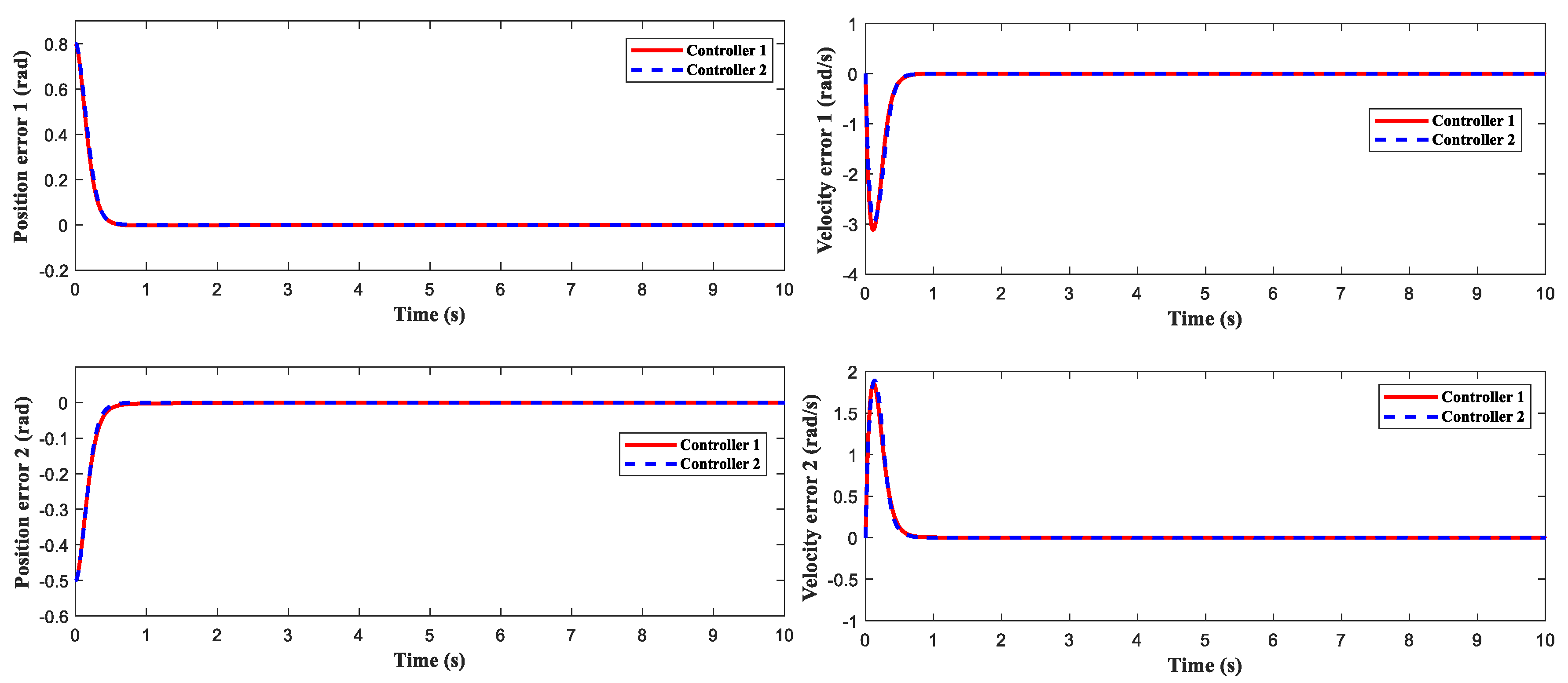
5. Simulation Comparisons

This section evaluates the feasibility of the control approach devised in this work through simulated verification with the following manipulator. Figure 2 depicts the simplified model of the 2-DOF rigid manipulator. The parameters related to the dynamics of the manipulator are given in detail below [31]. To demonstrate the effectiveness of the designed fixed-time sliding mode trajectory tracking control scheme with the adaptive fixed-time disturbance observer and the fixed-time saturation compensator, the other two controllers in [35,36] are introduced for making comparison. The parameter selection of the three controllers adopts the following unified standards and values.
M ( q ) = [ ( m 1 + m 2 ) r 1 2 + m 2 r 2 2 + J 1   + 2   m 2 r 1 r 2 cos ( q 2 )                               m 2 r 2 2 + m 2 r 1 r 2 cos ( q 2 )   m 2 r 2 2 + m 2 r 1 r cos ( q 2 )                                                                                                                       m 2 r 2 2 + J 2         ] C ( q , q ˙ ) = [ m 2 r 1 r 2 sin ( q 2 ) q ˙ 1                                                                             2 m 2 r 1 r 2 sin ( q 2 ) q ˙ 1                         0                                                                                                               m 2 r 1 r 2 sin ( q 2 ) q ˙ 2       ] G ( q ) = [ ( m 1 + m 2 ) r 1 g 1 cos ( q 1 )   + m 2 r 2 g 1 cos ( q 1 + q 2 )                                                     m 2 r 2 g 1 cos ( q 1 + q 2 ) ]
The parameters of the manipulator are as follows: J 1 = J 2 = 5.0   kg m , m 1 = 0.5   kg , m 2 = 1.5   kg , r 1 = 1.0   m , r 2 = 0.8   m , g = 9.8   m / s 2 , δ = 0.3 , μ 3 = 1.9 , M 0 = 0.65 I   Δ M ( q ) = 0.1 M ( q ) , Δ C ( q , q ˙ ) = 0.1 C ( q , q ˙ ) , Δ G ( q ) = 0.1 G ( q ) , ϖ 1 = 1.1 , ϖ 2 = 0.5 , C 1 = [ 5     , 0 ; 0 , 5 ] , C 2 = [ 5   , 0 ; 0 , 5 ] , K 1 = [ 5   , 0 ; 0 , 5 ] , K 2 = [ 5 , 0 ; 0 , 5 ] , and K 3 = [ 0.5   ; 0.5 ] .
The parameters of the AFSMDO are set as ε 1 = 80 , ε 2 = 80 , a 1 = 1.1 , a 2 = 0.5 , and ε 4 = 0.1 .
The design parameters of the fixed-time saturation compensator are set as α 1 = 0.15 , α 2 = 0.1 , α 3 = 0.01 , and K 4 = [ 0.1   , 0 ; 0.1 , 0 ] .
The expected trajectory of the manipulator is set as q d 1 = sin ( 3 t ) and q d 2 = cos ( 3 t ) ; the external disturbance is set to τ d 1 = 1 + 0.5 sin ( 2 π t ) and τ d 2 = 1 + 0.5 sin ( 2 π t ) .
Controller 1. The proposed global fixed-time sliding mode controller based on adaptive fixed-time disturbance observer with input compensation in this paper.
Controller 2. The fixed-time sliding mode controller based on a fixed-time disturbance observer [35].
τ 2 = M 0 ( q ) ( q ¨ d C 1 H e ˙ C 2 D e ˙ d ^ ) + C 0 ( q , q ˙ ) q ˙ + G 0 ( q )                 M 0 ( q ) ( K 1 S i g ϖ 1 ( s ) + K 2 S i g ϖ 2 ( s ) + K 3 s i g n ( s ) )
Controller 3. The global finite-time sliding mode controller with input saturation compensation [36].
τ 3 = M 0 ( q ) ( q ¨ d C 1 H e ˙ + d ^ K 2 S i g ϖ 2 ( s ) K 3 s i g n ( s ) K 4 M 0 ( q ) η ) + C 0 ( q , q ˙ ) q ˙ + G 0 ( q )
Controller 4. Traditional fixed time non-singular fast terminal sliding mode controller based on fixed time disturbance observer (ASMDO-NFTSMC).
τ 4 = M 0 q ¨ d M 0 d ^ M 0 ( k 1 l 1 | e | l 1 1 e ˙ + e ˙ ) k 2 l 2 | e ˙ | l 2 1 + C 0 ( q , q ˙ ) q ˙ + G 0 ( q )         M 0 ( q ) ( K 1 S i g ϖ 1 ( s ) + K 2 S i g ϖ 2 ( s ) + K 3 s i g n ( s ) )
The parameter designs of the NFTSMC sliding surface are as follows: l 1 = 2 , l 2 = 1.2 , k 1 = d i a g { 1 , 1 } , and k 2 = d i a g { 1 , 1 } .
The simulation verification of this article was carried out in two stages. First, in order to highlight the advantages of the control strategy proposed in this article, the initial joint angles of the manipulator system were selected as [1 rad, 2 rad] and [80 rad, 80 rad], and the above three controllers were simulated and verified, respectively. The second stage verified the effectiveness of the fixed time saturation compensator in compensating the input torque of the closed-loop system and reducing system chattering.
Figure 3, Figure 4, Figure 5, Figure 6 and Figure 7 display the outcomes of the simulation verification for the three control systems mentioned previously. The manipulator system trajectory tracking curve under the initial condition [1 rad, 2 rad] is shown in Figure 3a. Obviously, when the selected initial state approaches the origin, the three controllers enable the manipulator to effectively track the expected trajectory. The manipulator can complete the desired track tracking in 0.4 s under the control of controllers 1 and 2 and in 0.7 s under the control of controller 3. When the initial state is selected as [80 rad, 80 rad], the trajectory tracking accuracy of the manipulator is exhibited in Figure 3b. The aforementioned findings demonstrate that controllers 1 and 2 produce superior control results than controller 3, regardless of the manipulator starting position. The simulation graphs for tracking errors corresponding to the initial values [1 rad, 2 rad] and [80 rad, 80 rad] are given in Figure 4a and Figure 4b, respectively. Figure 5 indicates the tracking speed curves under different initial states. The corresponding velocity tracking errors are displayed in Figure 6. Figure 5a and Figure 6a independently display the velocity curve and velocity error curve for the initial condition of [1 rad, 2 rad]. Figure 5b and Figure 6b represent the velocity tracking curve and the velocity error curve under the initial state of [80 rad, 80 rad], respectively. This phenomenon confirms that our designed control strategy can rapidly and precisely follow the desired trajectory without requiring the initial condition of the system and has a better dynamic process than the finite-time control approach. Figure 7 exhibits the control torques of the three controllers. As opposed to controller 1 and controller 2, the initial control input of controller 3 is tiny, but it affects the control precision. Although the initial control torques of controller 1 and controller 2 are larger than that of controller 3, they are still within the range of the maximum control input that the manipulator can bear. Figure 8 shows the effect of interference observer of controller 1 and controller 3 on lumped disturbance estimation, respectively. By comparison, the fixed-time disturbance observer has better performance in disturbance tracking accuracy and response speed.
In order to more specifically demonstrate the superior performance of the controller proposed in this paper, the integrated absolute error (IAE), absolute average error (AAE), control input energy (ECI), control output energy average (AECI), and absolute input buffeting error (AICE) are used to compare the control effects of the three controllers. The specific mathematical expression is as follows.
| e i | I A E = k = 1 N | e i ( k ) |
| e i | A A E = 1 N k = 1 N | e i ( k ) |
| τ i | E C I = k = 1 N | τ i ( k ) |
| τ i | A E C I = 1 N k = 1 N | τ i ( k ) |
| Δ τ i | A I C E = 1 N k = 1 N 1 | τ i ( k + 1 ) τ i ( k ) |
where N is the total number of samples, and i is the number of joints.
Figure 9 and Figure 10 and Figure 11 and Figure 12 represent the IAE and AAE of three controllers under initial conditions [1 rad, 2 rad] and [80 rad, 80 rad], respectively. According to the numerical display of the stacked bar chart, compared with controller 2 and controller 3, the integral absolute error and absolute average error of controller 1 are significantly reduced, which indicates that the controller designed in this paper greatly improves the accuracy of the control system.
In order to more clearly demonstrate that FTSC can reduce the saturation input torque of the robotic arm and verify that the control scheme proposed in this study can effectively track different expected trajectories, the same expected trajectories and disturbance inputs as those in reference [31] are used for simulation verification. The design parameters of the fixed-time saturation compensator are reset as α 1 = 0.15 , α 2 = 0.1 , α 3 = 0.01 , and K 4 = [ 2 , 0   ; 0 , 2 ] .
q d 1 = 1.25 7 5 exp ( t ) + 7 20 exp ( 4 t ) q d 2 = 1.25 + exp ( t ) 1 4 exp ( 4 t ) τ d = [ 2 sin ( t ) + 0.5 sin ( 200 π t ) cos ( 2 t ) + 0.5 sin ( 200 π t ) ]
Figure 13 describes that the manipulator can effectively follow the intended trajectory under the control of controller 1 and controller 2. The speed tracking curve in Figure 14 shows that controller 1 and controller 2 also have a good and fast response performance under the same disturbance as [31]. The position error curve and speed error curve in Figure 15 further show that controller 1 and controller 2 also have good control accuracy for more complex target trajectories and external disturbances.
Figure 16 and Figure 17 illustrate the comparison of controller torque before and after introducing a saturation compensator into the controller of the two joints of the manipulator. The simulation curve clearly shows that by introducing a fixed-time saturation compensator, the manipulator can effectively reduce control inputs, making the control torque curve smoother and reducing torque chatter, which fully embodies the benefit of our designed control strategy.
The disturbance estimation curves of the two joints of the manipulator are shown in Figure 18. According to Figure 8 and Figure 8, it can be concluded that the adaptive disturbance observer designed in this study can achieve real-time, fast, and accurate disturbance estimation for different disturbances, improving the robustness of the system. Finally, Figure 19, Figure 20 and Figure 21 show ECI, AECI, and AICE stacked bar charts in controller 1 and controller 2 to verify the effect of the FTSC designed in this paper on the brake saturation of the control system. The AICE in Figure 21 measures the absolute control torque oscillation error of two controllers. The numerical results show that after introducing FTSC into the system, the absolute control torque buffeting errors of joint 1 and joint 2 decreased by 88.219% and 52.9%, respectively, indicating the effectiveness of the controller designed in this work.
The following simulation curves verify the superiority of the proposed NFSMC over the traditional NFTSMC. The target trajectory and disturbance are also in the form of Equation (62).
Figure 22 and Figure 23 show the trajectory tracking and velocity tracking curves of the controller in this paper and the nonsingular fast terminal sliding mode control design. Figure 24 and Figure 25 show the position tracking error and velocity tracking error of controller 1 and controller 4. The error curve indicates that the trajectory tracking and velocity tracking of controller 1, designed in this article, can converge to a small neighborhood of origin within 1 s, and the response speed of the controller has been greatly improved, which is significantly better than the tracking performance of controller 4.
To summarize, the control scheme described in this work has achieved the expected control objectives and demonstrated significant anti-interference ability and faster response speed coupled with satisfactory trajectory tracking accuracy, which is more favorable for practical application.

6. Conclusions

In this paper, the fixed-time trajectory tracking control problem for an input-saturated manipulator with exterior disturbances and model uncertainties has been researched. For the lumped disturbances in the manipulator system, the designed fixed-time disturbance observer could achieve fast and accurate estimation and compensation for the lumped disturbance, and the adaptive law could change the observer’s parameters to vary with the disturbance. The suggested nonsingular fixed-time sliding mode controller could converge the tracking error to an allowable range of error within a fixed amount of time and had the advantage of eliminating singularity. The introduction of the fixed-time saturation compensator greatly reduced the input torque chattering of the manipulator, making the proposed control strategy very suitable for practical industrial applications. Compared with the existing control method, the control scheme developed in this paper offers higher tracking accuracy, faster convergence speed, and less chattering. Future studies on this research will concentrate on how to accurately predict system stability time and develop the designed control algorithm into a predefined time sliding mode control.

Author Contributions

J.N. conceptualized the proposed system and is the author of the proposed controller design and control architecture. L.H. developed and executed the simulation program of the designed application. Data analyses were performed by X.L. The first draft of the manuscript was written by J.N., H.W. and C.S. analyzed and revised previous versions of the manuscript. All authors have read and agreed to the published version of the manuscript.

Funding

This work was supported by the National Natural Science Foundation of China (62203280, 62273213, 62073199), Natural Science Foundation of Shandong Province for Innovation and Development Joint Funds (ZR2022LZH001), Natural Science Foundation of Shandong Province (ZR2020MF095, ZR2022MF341), Taishan Scholarship Construction Engineering.

Data Availability Statement

The data that support the findings of this study are available from the corresponding author upon reasonable request.

Conflicts of Interest

The authors declare no conflict of interest.

References

  1. Aner, E.A.; Awad, M.I.; Shehata, O.M. Modeling and Trajectory Tracking Control for a Multi-Section Continuum Manipulator. J. Intell. Robot. Syst. 2023, 108, 49. [Google Scholar] [CrossRef]
  2. Pan, Q.; Li, Y.; Ma, B.; An, T.; Zhou, F. Event-triggered-based Decentralized Optimal Control of Modular Robot Manipulators Using RNN Identifier. J. Intell. Robot. Syst. 2022, 106, 55. [Google Scholar] [CrossRef]
  3. Cai, W.; Liu, Z.; Zhang, M.; Wang, C. Cooperative Artificial Intelligence for underwater robotic swarm. Robot. Auton. Syst. 2023, 164, 104410. [Google Scholar] [CrossRef]
  4. Yang, Y.; Cui, K.; Shi, D.; Mustafa, G.; Wang, J. PID control with PID event triggers: Theoretic analysis and experimental results. Control. Eng. Pract. 2022, 128, 105322. [Google Scholar] [CrossRef]
  5. Zhao, C.; Guo, L. Towards a theoretical foundation of PID control for uncertain nonlinear systems. Automatica 2022, 142, 110360. [Google Scholar] [CrossRef]
  6. Hernandez-Gonzalez, M.; Hernandez-Vargas, E. Discrete-time super-twisting controller using neural networks. Neurocomputing 2021, 447, 235–243. [Google Scholar] [CrossRef]
  7. Gassara, H.; Boukattaya, M.; El Hajjaji, A. Polynomial Adaptive Observer-Based Fault Tolerant Control for Time Delay Polynomial Fuzzy Systems Subject to Actuator Faults. Int. J. Fuzzy Syst. 2023, 25, 1327–1337. [Google Scholar] [CrossRef]
  8. Sun, C. Robust Finite Time Tracking Control for Robotic Manipulators Based on Nonsingular Fast Terminal Sliding Mode. Int. J. Control. Autom. Syst. 2022, 20, 3285–3295. [Google Scholar] [CrossRef]
  9. Yu, H.-P.; Wang, M.; Yang, J.; Xiong, J.-J. A Parallel-Structure-Based Sliding Mode Control for Trajectory Tracking of a Quadrotor UAV. J. Electr. Eng. Technol. 2023, 18, 3911–3924. [Google Scholar] [CrossRef]
  10. Ding, C.; Ding, S.; Wei, X.; Mei, K. Output feedback sliding mode control for path-tracking of autonomous agricultural vehicles. Nonlinear Dyn. 2022, 110, 2429–2445. [Google Scholar] [CrossRef]
  11. Chen, Y.; Jiang, C.; Dong, J.; Zhao, Z. Output feedback sliding mode control based on non-singular terminal sliding mode observer. Proc. Inst. Mech. Eng. Part I-J. Syst. Control Eng. 2023, 237, 939–949. [Google Scholar] [CrossRef]
  12. Yin, Z.; Yan, W.; Bintao, Z.; He, Z. Velocity-free adaptive nonsingular fast terminal sliding mode finite-time attitude tracking control for spacecraft. Asian J. Control. 2023, 25, 3687–3698. [Google Scholar] [CrossRef]
  13. Lian, S.; Meng, W.; Lin, Z.; Shao, K.; Zheng, J.; Li, H.; Lu, R. Adaptive Attitude Control of a Quadrotor Using Fast Nonsingular Terminal Sliding Mode. IEEE Trans. Ind. Electron. 2022, 69, 1597–1607. [Google Scholar] [CrossRef]
  14. Yao, M.; Xiao, X.; Tian, Y.; Cui, H. A fast terminal sliding mode control scheme with time-varying sliding mode surfaces. J. Frankl. Inst.-Eng. 2021, 358, 5386–5407. [Google Scholar] [CrossRef]
  15. Zhai, J.; Xu, G. A Novel Non-Singular Terminal Sliding Mode Trajectory Tracking Control for Robotic Manipulators. IEEE Trans. Circuits Syst. II Express Briefs 2021, 68, 391–395. [Google Scholar] [CrossRef]
  16. Lian, S.; Meng, W.; Shao, K.; Zheng, J.; Zhu, S.; Li, H. Full Attitude Control of a Quadrotor Using Fast Nonsingular Terminal Sliding Mode With Angular Velocity Planning. IEEE Trans. Ind. Electron. 2022, 70, 3975–3984. [Google Scholar] [CrossRef]
  17. Han, Q.; Tuo, X.; Tang, Y.; He, P. Finite-Time Attitude Cooperative Control of Multiple Unmanned Aerial Vehicles via Fast Nonsingular Terminal Sliding Mode Control. Wirel. Commun. Mob. Comput. 2022, 2022, 4324626. [Google Scholar] [CrossRef]
  18. Ding, S.; Park, J.H.; Chen, C.-C. Second-order sliding mode controller design with output constraint. Automatica 2020, 112, 108704. [Google Scholar] [CrossRef]
  19. Mi, W.; Luo, L.; Zhong, S. Fixed-Time Consensus Tracking for Multi-Agent Systems With a Nonholomonic Dynamics. IEEE Trans. Autom. Control 2023, 68, 1161–1168. [Google Scholar] [CrossRef]
  20. Cai, Z.; Huang, L.; Wang, Z. Novel Fixed-Time Stability Criteria for Discontinuous Nonautonomous Systems: Lyapunov Method With Indefinite Derivative. IEEE Trans. Cybern. 2022, 52, 4286–4299. [Google Scholar] [CrossRef]
  21. Ji, Y.; Chen, L.; Zhang, J.; Zhang, D.; Shao, X. Non-singular fixed-time pose tracking control for spacecraft with dead-zone input. Aircr. Eng. Aerosp. Technol. 2022, 94, 1390–1408. [Google Scholar] [CrossRef]
  22. Tian, Y.; Du, C.; Lu, P.; Jiang, Q.; Liu, H. Nonsingular fixed-time attitude coordinated tracking control for multiple rigid spacecraft. ISA Trans. 2022, 129, 243–256. [Google Scholar] [CrossRef] [PubMed]
  23. Zhang, J.; Xu, F.; Liu, X.; Gu, S.; Geng, H. Fixed-Time Dynamic Surface Control for Pneumatic Manipulator System With Unknown Disturbances. IEEE Robot. Autom. Lett. 2022, 7, 10890–10897. [Google Scholar] [CrossRef]
  24. Wei, X.; You, L.; Zhang, H.; Hu, X.; Han, J. Disturbance observer based control for dynamically positioned ships with ocean environmental disturbances and actuator saturation. Int. J. Robust Nonlinear Control. 2022, 32, 4113–4128. [Google Scholar] [CrossRef]
  25. Razmjooei, H.; Shafiei, M.H.; Palli, G.; Arefi, M.M. Non-linear Finite-Time Tracking Control of Uncertain Robotic Manipulators Using Time-Varying Disturbance Observer-Based Sliding Mode Method. J. Intell. Robot. Syst. 2022, 104, 36. [Google Scholar] [CrossRef]
  26. Sun, L.; Sun, G.; Jiang, J. Disturbance observer-based saturated fixed-time pose tracking for feature points of two rigid bodies. Automatica 2022, 144, 110475. [Google Scholar] [CrossRef]
  27. Ma, C.; Tang, Y.; Lei, M.; Jiang, D.; Luo, W. Trajectory tracking control for autonomous underwater vehicle with disturbances and input saturation based on contraction theory. Ocean Eng. 2022, 266, 112731. [Google Scholar] [CrossRef]
  28. Yan, Z.; Zhang, M.; Zhang, C.; Zeng, J. Decentralized formation trajectory tracking control of multi-AUV system with actuator saturation. Ocean Eng. 2022, 255, 111423. [Google Scholar] [CrossRef]
  29. Guo, G.; Li, P.; Hao, L.-Y. A New Quadratic Spacing Policy and Adaptive Fault-Tolerant Platooning With Actuator Saturation. IEEE Trans. Intell. Transp. Syst. 2022, 23, 1200–1212. [Google Scholar] [CrossRef]
  30. Huang, S.; Yang, Y.; Yan, Y.; Zhang, S.; Liu, Z. Observer-Based Robust Finite-Time Trajectory Tracking Control for a Stratospheric Satellite Subject to External Disturbance and Actuator Saturation. Int. J. Aerosp. Eng. 2022, 2022, 1601771. [Google Scholar] [CrossRef]
  31. Sai, H.; Xu, Z.; He, S.; Zhang, E.; Zhu, L.; Wang, C.; Li, X.; Cui, L.; Wang, Y.; Liang, M.; et al. Adaptive nonsingular fixed-time sliding mode control for uncertain robotic manipulators under actuator saturation. ISA Trans. 2022, 123, 46–60. [Google Scholar] [CrossRef] [PubMed]
  32. Lin, X.; Nie, J.; Jiao, Y.; Liang, K.; Li, H. Nonlinear adaptive fuzzy output-feedback controller design for dynamic positioning system of ships. Ocean Eng. 2018, 158, 186–195. [Google Scholar] [CrossRef]
  33. Zhang, L.; Wang, Y.; Hou, Y.; Li, H. Fixed-Time Sliding Mode Control for Uncertain Robot Manipulators. IEEE Access 2019, 7, 149750–149763. [Google Scholar] [CrossRef]
  34. Shi, R.; Zhang, X. Adaptive Fractional-order Non-singular Fast Terminal Sliding Mode Control Based on Fixed Time Observer. Proc. Inst. Mech. Eng. Part C-J. Eng. Mech. Eng. Sci. 2022, 236, 7006–7016. [Google Scholar] [CrossRef]
  35. Wu, C.; Yan, J.; Lin, H.; Wu, X.; Xiao, B. Fixed-time disturbance observer-based chattering-free sliding mode attitude tracking control of aircraft with sensor noises. Aerosp. Sci. Technol. 2021, 111, 106565. [Google Scholar] [CrossRef]
  36. Wang, H.; Zhang, Y.; Zhao, Z.; Tang, X.; Yang, J.; Chen, I.-M. Finite-time disturbance observer-based trajectory tracking control for flexible-joint robots. Nonlinear Dyn. 2021, 106, 459–471. [Google Scholar] [CrossRef]
Figure 1. Structure of the composite controller.
Axioms 12 00883 g001
Figure 2. Two-link manipulator.
Axioms 12 00883 g002
Figure 3. Position tracking comparison. (a) Position tracking curve at the initial values [1 rad, 2 rad]. (b) Position tracking curve at the initial values [80 rad, 80 rad].
Axioms 12 00883 g003
Figure 4. Position tracking error. (a) Position tracking error curve at the initial values [1 rad, 2 rad]. (b) Position tracking error curve at the initial values [80 rad, 80 rad].
Axioms 12 00883 g004
Figure 5. Joint velocity tracking comparison. (a) Joint velocity tracking curve at the initial values [1 rad, 2 rad]. (b) Joint velocity tracking curve at the initial values [80 rad, 80 rad].
Axioms 12 00883 g005
Figure 6. Joint velocity tracking error. (a) Joint velocity tracking error curve at the initial values [1 rad, 2 rad]. (b) Joint velocity tracking error curve at the initial values [80 rad, 80 rad].
Axioms 12 00883 g006
Figure 7. Control torques of joint 1 and 2.
Axioms 12 00883 g007
Figure 8. Disturbance observation.
Axioms 12 00883 g008
Figure 9. Integral absolute position error.
Axioms 12 00883 g009
Figure 10. Absolute average position error.
Axioms 12 00883 g010
Figure 11. Integral absolute position error.
Axioms 12 00883 g011
Figure 12. Absolute average position error.
Axioms 12 00883 g012
Figure 13. Joint 1 and joint 2 position tracking.
Axioms 12 00883 g013
Figure 14. Joint 1 and joint 2 velocity tracking.
Axioms 12 00883 g014
Figure 15. Position error and velocity error.
Axioms 12 00883 g015
Figure 16. Control torque of joint 1.
Axioms 12 00883 g016
Figure 17. Control torque of joint 2.
Axioms 12 00883 g017
Figure 18. Lumped disturbance estimation.
Axioms 12 00883 g018
Figure 19. Energy of control input.
Axioms 12 00883 g019
Figure 20. Average energy of control input.
Axioms 12 00883 g020
Figure 21. Absolute input torque chattering error.
Axioms 12 00883 g021
Figure 22. Position tracking comparison.
Axioms 12 00883 g022
Figure 23. Joint velocity tracking comparison.
Axioms 12 00883 g023
Figure 24. Position tracking error.
Axioms 12 00883 g024
Figure 25. Joint velocity tracking error.
Axioms 12 00883 g025
Disclaimer/Publisher’s Note: The statements, opinions and data contained in all publications are solely those of the individual author(s) and contributor(s) and not of MDPI and/or the editor(s). MDPI and/or the editor(s) disclaim responsibility for any injury to people or property resulting from any ideas, methods, instructions or products referred to in the content.

