Article

Inertial Iterative Algorithms for Split Variational Inclusion and Fixed Point Problems

by
Doaa Filali
1,
Mohammad Dilshad
2,*,
Lujain Saud Muaydhid Alyasi
2 and
Mohammad Akram
3,*
1
Department of Mathematical Science, College of Sciences, Princess Nourah Bint Abdulrahman University, P.O. Box 84428, Riyadh 11671, Saudi Arabia
2
Department of Mathematics, Faculty of Science, University of Tabuk, P.O. Box 741, Tabuk 71491, Saudi Arabia
3
Department of Mathematics, Faculty of Science, Islamic University of Madinah, P.O. Box 170, Madinah 42351, Saudi Arabia
*
Authors to whom correspondence should be addressed.
Axioms 2023, 12(9), 848; https://doi.org/10.3390/axioms12090848
Submission received: 9 July 2023 / Revised: 25 August 2023 / Accepted: 27 August 2023 / Published: 30 August 2023
(This article belongs to the Special Issue Nonlinear Functional Analysis in Natural Sciences)

Abstract

:
This paper aims to present two inertial iterative algorithms for estimating the solution of split variational inclusion ( S p VI s P ) and its extended version for estimating the common solution of ( S p VI s P ) and fixed point problem ( FPP ) of a nonexpansive mapping in the setting of real Hilbert spaces. We establish the weak convergence of the proposed algorithms and strong convergence of the extended version without using the pre-estimated norm of a bounded linear operator. We also exhibit the reliability and behavior of the proposed algorithms using appropriate assumptions in a numerical example.

1. Introduction

The split feasibility problems ( S p FP ) , due to Censor and Elfving [1], have ample applications in medical science. Therefore, ( S p FP ) has been widely used over the past twenty years in the design of intensity-modulation therapy treatments and other areas of applied sciences, see, e.g., [2,3,4,5]. Censor et al. [6,7] merged the variational inequality problem ( VI t P ) and ( S p FP ) , and a different kind of problem came to existence known as split variational inequality problem ( S p VI t P ) defined as:
Find out l * Q 1 such that l * VI t P ( F 1 ; Q 1 )   and   B ( l * ) VI t P ( F 2 ; Q 2 ) ,
where Q 1 and Q 2 are subsets of Hilbert spaces X 1 and X 2 , respectively, B : X 1 X 2 is a bounded linear operator, F 1 : X 1 X 1 and F 2 : X 2 X 2 are two operators, VI t P ( F 1 ; Q 1 ) = { q C : F 1 ( q ) , p q 0 , p Q 1 } and VI t P ( F 2 ; Q 2 ) = { r Q 2 : F 2 ( r ) , s r 0 , s Q 2 } .
Moudafi [8] extended S p VI t P into a split monotone variational inclusion problem ( S p MVI s P ) defined as:
Find out l * X 1 such that l * VI s P ( F 1 ; A 1 ; X 1 )   and   B ( l * ) VI s P ( A 2 ; F 2 ; X 2 ) ,
where A 1 : X 1 2 X 1 and A 2 : X 2 2 X 2 are set-valued mappings on Hilbert spaces X 1 and X 2 , respectively, VI s P ( F 1 , A 1 ; X 1 ) = { p X 1 : 0 F 1 ( p ) + A 1 ( p ) } and VI s P ( F 2 , A 2 ; X 2 ) = { q X 2 : 0 F 2 ( q ) + A 2 ( q ) } . Moudafi [8] proposed the following iterative scheme for ( S p MVI s P ) . Let μ > 0 , choose any starting point z 0 X 1 and compute
z n + 1 = V [ z n + λ B * ( W I ) B z n ] ,
where B * is an adjoint operator of B, λ ( 0 , 1 / R ) with R being the spectral radius of the operator B * B , V = R μ A 1 ( I μ F 1 ) = ( I + μ A 1 ) 1 ( I μ F 1 ) and W = R μ A 2 ( I μ F 2 ) = ( I + μ A 2 ) 1 ( I μ F 2 ) .
If F 1 = F 2 = 0 , then ( S p MVI s P ) turns into the split inclusion problem (in short, ( S p VI s P ) suggested and discussed by Byrne et al. [9]:
Find out l * X 1 such that l * VI s P ( A 1 ; X 1 )   and   B ( l * ) VI s P ( A 2 ; X 2 ) ,
where VI s P ( A 1 ; X 1 ) = { p X 1 : 0 A 1 ( p ) } and VI s P ( A 2 ; X 2 ) = { q X 2 : 0 A 2 ( q ) } , A 1 , A 2 are the same as in (2). Moreover, Byrne et al. [9] suggested the following iterative scheme for ( S p VI s P ) . Let μ > 0 and select a starting point z 0 X 1 ; then, compute
z n + 1 = R μ A 1 [ z n + λ B * ( I R μ A 2 ) B z n ] ,
where B * is the adjoint operator of B, R = B * B = B 2 , λ ( 0 , 2 / R ) and R μ A 1 , R μ A 2 are the resolvents of monotone mappings A 1 , A 2 , respectively. It is obvious to see that l * solves ( S p VI s P ) if and only if l * = R μ A 1 [ l * + λ B * ( I R μ A 2 ) B l * ] . Kazmi and Rizvi [10] studied the following iterative scheme for calculating the common solutions of ( S p VI s P ) and ( FPP ) of a nonexpansive mapping S. For z 0 X 1 , compute
y n = R μ A 1 [ z n + λ B * ( R μ A 2 I ) B z n ] , z n + 1 = ζ n f ( z n ) + ( 1 ζ n ) S y n ,
where f is contraction and λ ( 0 , 2 B 2 ) . By extending the work of Kazmi and Rizvi [10], Dilshad et al. [11] discussed the common solution of ( S p VI s P ) and the fixed point of a finite collection of nonexpansive mappings. Sitthithakerngkiet et al. [12] investigated the common solutions of ( S p VI s P ) and a fixed point of a countably infinite collection of nonexpansive mappings and proposed and discussed the following method. For z 0 X 1 , compute
y n = R μ A 1 [ z n + λ B * ( R μ A 2 I ) B z n ] , z n + 1 = ζ n u + ξ n z n + [ ( 1 ξ n ) I ζ n D ] W n y n , n 1 ,
where u X 1 is arbitrary, and W n is W-mapping, which is created by an infinite collection of nonexpansive mappings. Furthermore, Akram et al. [13] modify the method discussed in [10] and investigate the common solution of ( S p VI s P ) and ( FPP ) :
y n = z n λ ( I R μ 1 A 1 ) z n + B * ( I R μ 2 A 2 ) B z n , z n + 1 = ζ n f ( z n ) + ( 1 ζ n ) S ( y n ) ,
where λ = 1 1 + B 2 , ζ n ( 0 , 1 ) satisfying lim n ζ n = 0 , n = 1 ζ n = and n = 1 | ζ n ζ n 1 | < . Some results related to ( S p VI s P ) and ( FPP ) can be found in [14,15,16,17,18,19] and the references therein.
It is noted that the step size depending upon the norm B * B is commonly used in the above-mentioned iterative schemes. To skip this restruction, a new type of iterative method with a self-adaptive step size has been invented. López et al. [20] composed a relaxed iterative method for ( S p FP ) with a self-adaptive step size. Dilshad et al. [21] studied the ( S p VI s P ) without using a pre-calculated norm B . Some useful related work can be found in [22,23,24,25,26] and the references therein.
In recent years, great efforts have been made to speed up various algorithms. The inertia term as one of the speed-up techniques has been studied by many scientists because of its simple form and good speed-up effect. Recall that using the concepts of implicit descritization for the derivatives, Alvarez and Attouch [27] have developed the inertial proximal point method, which can be expressed as
z n + 1 = R μ A [ z n + ϕ n ( z n z n 1 ) ] ,
where A is monotone mapping, R μ A is the resolvent of A and μ > 0 . Such types of schemes have a better convergence rate, and hence, this scheme was modified and applied to solve numerous nonlinear problems; see [28,29,30,31,32,33,34] and the references therein.
Following the above-mentioned inertial method, we consider two inertial iterative algorithms for approximating the solution of ( S p VI s P ) and common solutions of ( S p VI s P ) and ( FPP ) of a nonexpansive mapping.
The next section contains some theory and auxiliary results which are helpful in the proof of the main results. In Section 3, we explain two self-adaptive inertial iterative methods. Section 4 is focused on the proof of the main results discussing the solution of ( S p VI s P ) and a common solution of ( S p VI s P ) and ( FPP ) . At last, we illustrate a numerical example in favor of the proposed iterative algorithms showing their behavior and reliability.

2. Preliminaries

Assume that ( X , · ) is a real Hilbert space with the inner product · , · . The strong convergence of the real sequence { z n } to z is indicated by z n z and the weak convergence is indicated by z n z . If { z n } is a sequence in X, ω w ( z n ) indicates the weak ω -limit set of { z n } , that is
ω w ( z n ) = { z H : z n j z as j where z n j is a subsequnce of z n } .
We know that for some z X , there exists a unique nearest point in Q denoted by P Q z such that
z P Q z z v , v Q .
P Q z is called the projection of z onto Q X , which satisfies
z v , P Q z P C v P Q z P Q v 2 , z , v X .
Moreover, P Q z is identified by the fact
P Q z = x z v , v x 0 , v Q .
For all p , q , r in Hilbert space X, ϕ , φ , ψ [ 0 , 1 ] such that ϕ + φ + ψ = 1 ; then, we have the following equality and inequality
ϕ p + φ q + ψ r 2 = ϕ p 2 + φ q 2 + ψ r 2 ϕ φ p q 2 φ ψ q r w 2 ψ ϕ p r 2 ,
and
p + q 2 p 2 + 2 q , p + q .
Definition 1.
A mapping F : X X is called
(i) 
Contraction, if F ( p ) F ( q ) κ p q , p , q X , κ ( 0 , 1 ) ;
(ii) 
Nonexpansive, if F ( p ) F ( q ) p q , p , q X ;
(iii) 
Firmly nonexpansive, if F ( p ) F ( q ) 2 p q , F ( p ) F ( q ) , p , q X ;
(iv) 
τ-inverse strongly monotone, if there exists τ > 0 such that
F ( p ) F ( q ) , p q τ F ( p ) F ( q ) 2 , p , q X .
Definition 2.
Let A : X 2 X be a set valued mapping. Then
(i) 
The mapping A is called monotone if u v , p q 0 , u , v X , u A ( p ) , v A ( q ) ;
(ii) 
G r a p h ( A ) = { ( u , p ) X × X : u A ( p ) } ;
(iii) 
The mapping A is called maximal monotone if G r a p h ( A ) is not properly contained in the graph of any other monotone operator.
Lemma 1
([35]). If { s n } is a sequence of non-negative real numbers such that
s n + 1 ( 1 ξ n ) s n + δ n , n 0 ,
where { ξ n } is a sequence in ( 0 , 1 ) and { δ n } is a sequence of real numbers such that
(i) 
n = 1 ξ n = ;
(ii) 
lim sup n δ n ξ n 0 or n = 1 | δ n | < .
Then lim n s n = 0 .
Lemma 2
([36]). In a Hilbert space X,
(i) 
a mapping A : X X is τ-inverse strongly monotone if and only if I τ A is firmly nonexpansive for τ > 0 .
(ii) 
If A : X 2 X is monotone and R μ A is the resolvent of A, then R μ A and I R μ A are firmly nonexpansive for μ > 0 .
(iii) 
If A : X X is nonexpansive, then I A is demiclosed at zero and if A is firmly nonexpansive, then I A is firmly nonexpansive.
Lemma 3
([37]). Let { ψ n } be a bounded sequence in Hilbert space X. Assume there exists a subset Q and Q X satisfying the properties
(i) 
lim n ψ n z exists, z Q ,
(ii) 
ω w ( ψ n ) Q .
Then, there exists z * C such that ψ n z * .
Lemma 4
([38]). Let Γ n be a sequence of real numbers that does not decrease at infinity in the sense that there exists a subsequence Γ n k of Γ n such that Γ n k < Γ n k + 1 for all k 0 . In addition, consider the sequence of integers { σ ( n ) } n n 0 defined by
σ ( n ) = max { k n : Γ k Γ k + 1 } .
Then, { σ ( n ) } n n 0 is a nondecreasing sequence verifying lim n σ ( n ) = and n n 0 ,
max { Γ σ ( n ) , Γ ( n ) } Γ σ ( n ) + 1 .
Lemma 5
([38]). Assume that { s n } is a non-negative sequence of real numbers satisfying
(i) 
s n + 1 s n δ n ( s n s n 1 ) + θ n ;
(ii) 
n = 1 θ n < ;
(iii) 
δ n [ 0 , κ ] , where κ [ 0 , 1 ) .
Then, { s n } is convergent and n = 1 ( s n + 1 s n ) < , where [ h ] + = max { h , 0 } for any h R .

3. Inertial Iterative Methods

Suppose that X 1 and X 2 are real Hilbert spaces and A 1 : X 1 2 X 1 , A 2 : X 2 2 X 2 are monotone mappings; R μ 1 A 1 , R μ 2 A 2 are the resolvents of A 1 and A 2 , respectively. We assume that Λ Fix ( F ) , where Λ denotes the solution set of S p VI s P and Fix ( F ) denotes the fixed point set of FPP . First, we suggest the following iterative algorithm for S p VI s P .
Algorithm 1.
Choose ϕ such that 0 ϕ < 1 and let δ n be a positive sequence satisfying  n = 1 δ n < .
  • Iterative Step: Given arbitrary x 0 , and x 1 , for n 1 , choose 0 < ϕ n < ϕ ˜ n , where
    ϕ ˜ n = min δ n x n x n 1 , ϕ , if x n x n 1 , ϕ , otherwise .
Compute
v n = x n + ϕ n ( x n x n 1 ) , u n = v n σ n ( I R μ 1 A 1 ) ( v n ) , x n + 1 = u n ϱ n B * ( I R μ 2 A 2 ) ( B u n ) ,
where σ n and ϱ n are defined as
σ n = τ n ( I R μ 1 A 1 ) ( v n ) 2 ( I R μ 1 A 1 ) ( v n ) 2 + B * ( I R μ 2 A 2 ) ( B v n ) 2 , if ( I R μ 1 A 1 ) ( v n ) 2 + B * ( I R μ 2 A 2 ) ( B v n ) 2 0 0 , o t h e r w i s e
and
ϱ n = τ n ( I R μ 2 A 2 ) ( B u n ) 2 ( I R μ 1 A 1 ) ( u n ) 2 + B * ( I R μ 2 A 2 ) ( B u n ) 2 , if ( I R μ 1 A 1 ) ( u n ) 2 + B * ( I R μ 2 A 2 ) ( B u n ) 2 0 0 , o t h e r w i s e
where μ 1 > 0 , μ 2 > 0 and τ n ( 0 , 2 ) .
Algorithm 2.
Choose ϕ such that 0 ϕ < 1 and let δ n be a positive sequence satisfying n = 1 δ n < .
  • Iterative Step: Given arbitrary x 0 , and x 1 , for n 1 , choose 0 < ϕ n < ϕ ˜ n , where
    ϕ ˜ n = min δ n x n x n 1 , ϕ , if x n x n 1 , ϕ , otherwise .
Compute
v n = x n + ϕ n ( x n x n 1 ) , u n = v n σ n ( I R μ 1 A 1 ) ( v n ) , w n = u n ϱ n B * ( I R μ 2 A 2 ) ( B u n ) , x n + 1 = ( 1 ζ n ξ n ) u n + ζ n F ( w n ) .
where σ n and ϱ n are defined as
σ n = τ n ( I R μ 1 A 1 ) ( v n ) 2 ( I R μ 1 A 1 ) ( v n ) 2 + B * ( I R μ 2 A 2 ) ( B v n ) 2 , if ( I R μ 1 A 1 ) ( v n ) 2 + B * ( I R μ 2 A 2 ) ( B v n ) 2 0 0 , o t h e r w i s e
and
ϱ n = τ n ( I R μ 2 A 2 ) ( B u n ) 2 ( I R μ 1 A 1 ) ( u n ) 2 + B * ( I R μ 2 A 2 ) ( B u n ) 2 , if ( I R μ 1 A 1 ) ( u n ) 2 + B * ( I R μ 2 A 2 ) ( B u n ) 2 0 0 , o t h e r w i s e
where ζ n , ξ n ( 0 , 1 ) , μ 1 > 0 , μ 2 > 0 , and τ n ( 0 , 2 ) .
Remark 1.
It is not difficult to show that if ( I R μ 1 A 1 ) ( u n ) 2 + B * ( I R μ 2 A 2 ) ( B u n ) 2 = 0 or ( I R μ 1 A 1 ) ( v n ) 2 + B * ( I R μ 2 A 2 ) ( B v n ) 2 = 0 for some n 0 , then x n Λ . In this case, the iteration process ended after a finite number of iterations. We suppose that the proposed algorithms generate infinite sequences which do not end in a finite number of terms.
Remark 2.
From the selection of δ n , such that n = 1 δ n < , we can conclude that lim n ϕ n x n x n 1 = 0 .
Remark 3.
By using the definitions of resolvent of monotone mappings A 1 and A 2 , we can easily obtain that l Λ if and only if R μ 1 A 1 ( l ) = l * and R μ 2 A 2 ( B l ) = B ( l ) .

4. Main Results

Theorem 1.
Let X 1 , X 2 be real Hilbert spaces; A 1 : X 1 2 X 1 , A 2 : X 2 2 X 2 be maximal monotone mappings and B : X 1 X 2 be a bounded linear operator. If τ n ( 0 , 2 ) and ζ n , ξ n ( 0 , 1 ) such that
lim n ξ n = 0 , n = 0 ξ n = , lim n ( 1 ζ n ξ n ) ζ n > 0 , inf n τ n ( 2 τ n ) > 0 .
Then, the sequence { x n } generated from Algorithm 1 converges weakly to a point z Λ .
Proof. 
Let l Λ , then ( I R μ 1 A 1 ) ( l ) = 0 . Since resolvent operator R μ 1 A 1 is firmly nonexpansive, hence, so is ( I R μ 1 A 1 ) for μ 1 > 0 , then by Algorithm 1 and (10), we have
u n l 2 = v n σ n ( I R μ 1 A 1 ) ( v n ) l 2 v n l 2 + σ n 2 ( I R μ 1 A 1 ) ( v n ) 2 2 σ n ( I R μ 1 A 1 ) ( v n ) , v n l = v n l 2 + σ n 2 ( I R μ 1 A 1 ) ( v n ) 2 2 σ n ( I R μ 1 A 1 ) ( v n ) ( I R μ 1 A 1 ) ( l ) , v n l v n l 2 + σ n 2 ( I R μ 1 A 1 ) ( v n ) 2 2 σ n ( I R μ 1 A 1 ) ( v n ) ( I R μ 1 A 1 ) ( l ) 2 = v n l 2 + ( σ n 2 2 σ n ) ( I R μ 1 A 1 ) ( v n ) 2 .
Now, using (12), we estimate that
( σ n 2 2 σ n ) ( I R μ 1 A 1 ) ( v n ) 2 = ( I R μ 1 A 1 ) ( v n ) 2 [ τ n 2 ( I R μ 1 A 1 ) ( v n ) 4 ( I R μ 1 A 1 ) ( v n ) 2 + B * ( I R μ 2 A 2 ) ( B v n ) 2 2 2 τ n ( I R μ 1 A 1 ) ( v n ) 2 ( I R μ 1 A 1 ) ( v n ) 2 + B * ( I R μ 2 A 2 ) ( B v n ) 2 ]
= ( I R μ 1 A 1 ) ( v n ) 4 τ n 2 ( I R μ 1 A 1 ) ( v n ) 2 2 τ n ( ( I R μ 1 A 1 ) ( v n ) 2 + B * ( I R μ 2 A 2 ) ( B v n ) 2 ) ( I R μ 1 A 1 ) ( v n ) 2 + B * ( I R μ 2 A 2 ) ( B v n ) 2 2 ( I R μ 1 A 1 ) ( v n ) 4 ( τ n 2 2 τ n ) ( ( I R μ 1 A 1 ) ( v n ) 2 + B * ( I R μ 2 A 2 ) ( B v n ) 2 ) ( I R μ 1 A 1 ) ( v n ) 2 + B * ( I R μ 2 A 2 ) ( B v n ) 2 2 = ( τ n 2 2 τ n ) ( I R μ 1 A 1 ) ( v n ) 4 ( I R μ 1 A 1 ) ( v n ) 2 + B * ( I R μ 2 A 2 ) ( B v n ) 2 .
From (18) and (19), we obtain
u n l 2 v n l 2 + ( τ n 2 2 τ n ) ( I R μ 1 A 1 ) ( v n ) 4 ( I R μ 1 A 1 ) ( v n ) 2 + B * ( I R μ 2 A 2 ) ( B v n ) 2 .
Since ( I R μ 2 A 2 ) is firmly nonexpasive and using ( I R μ 2 A 2 ) ( B l ) = 0 and (10), we estimate
x n + 1 l 2 = u n ϱ n ( I R μ 2 A 2 ) ( B u n ) l 2 u n l 2 + ϱ n 2 ( I R μ 2 A 2 ) ( B u n ) 2 2 ϱ n ( I R μ 2 A 2 ) ( B u n ) , u n l = u n l 2 + ϱ n 2 ( I R μ 2 A 2 ) ( B u n ) 2 2 ϱ n ( I R μ 2 A 2 ) ( B u n ) ( I R μ 2 A 2 ) ( B l ) , u n l = u n l 2 + ϱ n 2 ( I R μ 2 A 2 ) ( B u n ) 2 2 ϱ n ( I R μ 1 A 1 ) ( B u n ) 2 = u n l 2 + ( ϱ n 2 2 ϱ n ) J λ 1 A 2 ( B u n ) 2 .
By (13), it turns out that
( ϱ n 2 2 ϱ n ) ( I R μ 2 A 2 ) ( B u n ) 2 = ( I R μ 2 A 2 ) ( B u n ) 2 [ τ n 2 ( I R μ 2 A 2 ) ( B u n ) 4 ( I R μ 1 A 1 ) ( u n ) 2 + B * ( I R μ 2 A 2 ) ( B u n ) 2 2 2 τ n ( I R μ 2 A 2 ) ( B u n ) 2 ( I R μ 1 A 1 ) ( u n ) 2 + B * ( I R μ 2 A 2 ) ( B u n ) 2 ] = ( I R μ 2 A 2 ) ( B u n ) 4 × τ n 2 ( I R μ 2 A 2 ) ( B u n ) 2 2 τ n ( ( I R μ 1 A 1 ) ( u n ) 2 + B * ( I R μ 2 A 2 ) ( B u n ) 2 ) ( I R μ 1 A 1 ) ( u n ) 2 + B * ( I R μ 2 A 2 ) ( B u n ) 2 2 ( I R μ 2 A 2 ) ( B u n ) 4 ( τ n 2 2 τ n ) ( I R μ 1 A 1 ) ( u n ) 2 + B * ( I R μ 2 A 2 ) ( B u n ) 2 ( I R μ 1 A 1 ) ( u n ) 2 + B * ( I R μ 2 A 2 ) ( B u n ) 2 2 = ( τ n 2 2 τ n ) ( I R μ 2 A 2 ) ( B u n ) 4 ( I R μ 1 A 1 ) ( u n ) 2 + B * ( I R μ 2 A 2 ) ( B u n ) 2 .
It follows from (21) and (22) that
x n + 1 l 2 u n l 2 + ( τ n 2 2 τ n ) ( I R μ 2 A 2 ) ( B u n ) 4 ( I R μ 1 A 1 ) ( u n ) 2 + B * ( I R μ 2 A 2 ) ( B u n ) 2 .
Combining (20) and (23), we obtain
x n + 1 l 2 v n l 2 + τ n ( τ n 2 ) ( I R μ 1 A 1 ) ( v n ) 4 ( I R μ 1 A 1 ) ( v n ) 2 + B * ( I R μ 2 A 2 ) ( B v n ) 2 + τ n ( τ n 2 ) ( I R μ 2 A 2 ) ( B u n ) 4 ( I R μ 1 A 1 ) ( u n ) 2 + B * ( I R μ 2 A 2 ) ( B u n ) 2
By using the Cauchy–Schwartz inequality, we observe that
v n l 2 = x n l + ϕ n ( x n x n 1 ) 2 = x n l 2 + 2 ϕ n x n x n 1 , x n l + ϕ n 2 x n x n 1 2 . x n l 2 + 2 ϕ n x n x n 1 x n l + ϕ n x n x n 1 2 .
Since 2 x n x n 1 x n l = x n x n 1 2 + x n l 2 ( x n x n 1 ) ( x n l ) 2 , we get
v n l 2 x n l 2 + 2 ϕ n x n x n 1 2 + ϕ n x n l 2 x n 1 l 2 .
From (25) and (24), we obtain
x n + 1 l 2 x n l 2 + 2 ϕ n x n x n 1 2 + ϕ n x n l 2 x n 1 l 2 + τ n ( τ n 2 ) ( I R μ 1 A 1 ) ( v n ) 4 ( I R μ 1 A 1 ) ( v n ) 2 + B * ( I R μ 2 A 2 ) ( B v n ) 2 + τ n ( τ n 2 ) ( I R μ 2 A 2 ) ( B u n ) 4 ( I R μ 1 A 1 ) ( u n ) 2 + B * ( I R μ 2 A 2 ) ( B u n ) 2 .
Since, τ n ( 0 , 2 ) , that is τ n 2 < 0 , we obtain
( x n + 1 l 2 x n l 2 ) ϕ n x n l 2 x n 1 l 2 + 2 ϕ n x n x n 1 2
Applying Lemma 5, we deduce that the limit x n l exists, which guarantees the boundednesss of sequence { x n } and hence { u n } and { v n } . From (26), it follows that n = 1 ϕ n x n l 2 x n 1 l 2 < and
n = 1 ( I R μ 1 A 1 ) ( v n ) 4 ( I R μ 1 A 1 ) ( v n ) 2 + B * ( I R μ 2 A 2 ) ( B v n ) 2 + ( I R μ 2 A 2 ) ( B u n ) 4 ( I R μ 1 A 1 ) ( u n ) 2 + B * ( I R μ 2 A 2 ) ( B u n ) 2 < ,
which concludes
lim n ( I R μ 1 A 1 ) ( v n ) 4 ( I R μ 1 A 1 ) ( v n ) 2 + B * ( I R μ 2 A 2 ) ( B v n ) 2 + ( I R μ 2 A 2 ) ( B u n ) 4 ( I R μ 1 A 1 ) ( u n ) 2 + B * ( I R μ 2 A 2 ) ( B u n ) 2 = 0 ,
hence
lim n ( I R μ 1 A 1 ) ( v n ) 4 ( I R μ 1 A 1 ) ( v n ) 2 + B * ( I R μ 2 A 2 ) ( B v n ) 2 = 0 , lim n ( I R μ 2 A 2 ) ( B u n ) 4 ( I R μ 1 A 1 ) ( u n ) 2 + B * ( I R μ 2 A 2 ) ( B u n ) 2 = 0 ,
which concludes that
lim n ( I R μ 1 A 1 ) ( v n ) = lim n ( I R μ 2 A 2 ) ( B u n ) = 0 .
It remains to show that ω w ( x n ) Λ . Let l ω w ( x n ) and { x n k } be a subsequence of { x n } so that x n k l , as k . Applying (27) and Remark 2, in Algorithm 1, it follows that
x n v n = ϕ n x n x n 1 0 , n
x n u n = x n [ v n σ n ( I R μ 1 A 1 ) ( v n ) ] x n v n + σ n ( I R μ 1 A 1 ) ( v n ) x n v n + τ n ( I R μ 1 A 1 ) ( v n ) 3 ( I R μ 1 A 1 ) ( v n ) 2 + B * ( I R μ 2 A 2 ) ( B v n ) 2 0 , n
and
v n u n x n u n + v n x n 0 , n .
Hence, there exist subsequences { u n k } and { v n k } of { u n } and { v n } , respectively, which converge to l . From (27), we obtain
lim k ( I R μ 1 A 1 ) ( v n k ) = lim k ( I R μ 1 A 1 ) ( l ) = 0 , lim k ( I R μ 2 A 2 ) ( B u n k ) = lim k ( I R μ 2 A 2 ) ( B l ) = 0 ,
which imply that l A 1 1 ( 0 ) and B ( l ) A 2 1 ( 0 ) . □
Theorem 2.
Let X 1 , X 2 be real Hilbert spaces; and let A 1 : X 1 2 X 1 , A 2 : X 2 2 X 2 be set-valued maximal monotone mappings. If { ζ n } , { ξ n } are real sequences in ( 0 , 1 ) , τ n ( 0 , 2 ) and
lim n ξ n = 0 , n = 0 ξ n = , lim n ( 1 ζ n ξ n ) ζ n > 0 , inf n τ n ( 2 τ n ) > 0 .
Then, the sequence { x n } obtained from Algorithm 2 converges strongly to l = P Λ Fix ( F ) ( 0 ) .
Proof. 
Let l = P Λ Fix ( F ) ( 0 ) . From Algorithm 2, we have
v n l = x n + ϕ n ( x n x n 1 ) l ( 1 ϕ n ) x n l + ϕ n x n 1 l max { x n l , x n 1 l } ,
and
x n + 1 l = ( 1 ζ n ξ n ) u n + ζ n F ( w n ) l ( 1 ζ n ξ n ) u n l + + ζ n F ( w n ) l + ξ n l ( 1 ζ n ξ n ) u n l + + ζ n w n l + ξ n l ( 1 ξ n ) v n l + ξ n l ( 1 ξ n ) ( 1 ϕ n ) x n l + ϕ n x n 1 l + ξ n l max { x n l , x n 1 l , l } max { x 0 l , x 1 l , l } ,
which shows that { x n } is bounded and hence the { v n } , { u n } , and { w n } are bounded. From (20) and (23) of the proof of Theorem 1, we have
u n l 2 v n l 2 + ( τ n 2 2 τ n ) ( I R μ 1 A 1 ) ( v n ) 4 ( I R μ 1 A 1 ) ( v n ) 2 + B * ( I R μ 2 A 2 ) ( B v n ) 2 v n l 2 .
w n l 2 u n l 2 + ( τ n 2 2 τ n ) ( I R μ 2 A 2 ) ( B u n ) 4 ( I R μ 1 A 1 ) ( u n ) 2 + B * ( I R μ 2 A 2 ) ( B u n ) 2 u n l 2 .
Now,
x n + 1 l 2 = ( 1 ζ n ξ n ) u n + ζ n F ( w n ) l 2 = ( 1 ζ n ξ n ) ( u n l ) + ζ n ( F ( w n ) l ) + ξ n ( l ) 2 ( 1 ζ n ξ n ) u n l 2 + ζ n F ( w n ) l 2 + ξ n l 2 ζ n ( 1 ζ n ξ n ) u n F ( w n ) 2 = ( 1 ζ n ξ n ) u n l 2 + ζ n w n l 2 + ξ n l 2 ζ n ( 1 ζ n ξ n ) u n F ( w n ) 2 .
Combining (30)–(32), we obtain
x n + 1 l 2 ( 1 ζ n ξ n ) v n l 2 + ( τ n 2 2 τ n ) ( I R μ 1 A 1 ) ( v n ) 4 ( I R μ 1 A 1 ) ( v n ) 2 + B * ( I R μ 2 A 2 ) ( B v n ) 2 + ζ n u n l 2 + ( τ n 2 2 τ n ) ( I R μ 2 A 2 ) ( B u n ) 4 ( I R μ 1 A 1 ) ( u n ) 2 + B * ( I R μ 2 A 2 ) ( B u n ) 2 + ξ n l 2 ζ n ( 1 ζ n ξ n ) u n F ( w n ) 2 ( 1 ζ n ξ n ) v n l 2 + ζ n u n l 2 ζ n ( 1 ζ n ξ n ) u ) F ( w n ) 2 ( 1 ζ n ξ n ) ( τ n 2 2 τ n ) ( I R μ 1 A 1 ) ( v n ) 4 ( I R μ 1 A 1 ) ( v n ) 2 + B * ( I R μ 2 A 2 ) ( B v n ) 2 ζ n ( τ n 2 2 τ n ) ( I R μ 2 A 2 ) ( B u n ) 4 ( I R μ 1 A 1 ) ( u n ) 2 + B * ( I R μ 2 A 2 ) ( B u n ) 2 + ξ n l 2
( 1 ξ n ) x n l 2 + 2 ϕ n x n x n 1 2 + ϕ n x n l 2 x n 1 l 2 ζ n ( 1 ζ n ξ n ) u n F ( w n ) 2 + ( 1 ζ n ξ n ) ( τ n 2 2 τ n ) ( I R μ 1 A 1 ) ( v n ) 4 ( I R μ 1 A 1 ) ( v n ) 2 + B * ( I R μ 2 A 2 ) ( B v n ) 2 + ζ n ( τ n 2 2 τ n ) ( I R μ 2 A 2 ) ( B u n ) 4 ( I R μ 1 A 1 ) ( u n ) 2 + B * ( I R μ 2 A 2 ) ( B u n ) 2 + ξ n l 2 x n l 2 + 2 ϕ n x n x n 1 2 + ϕ n x n l 2 x n 1 l 2 ζ n ( 1 ζ n ξ n ) u n F ( w n ) 2 + ( 1 ζ n ξ n ) τ n ( 2 τ n ) ( I R μ 1 A 1 ) ( v n ) 4 ( I R μ 1 A 1 ) ( v n ) 2 + B * ( I R μ 2 A 2 ) ( B v n ) 2 + ζ n τ n ( 2 τ n ) ( I R μ 2 A 2 ) ( B u n ) 4 ( I R μ 1 A 1 ) ( u n ) 2 + B * ( I R μ 2 A 2 ) ( B u n ) 2 + ξ n l 2 .
Two possible cases occur.
Case I. Suppose the sequence { x n l } is nonincreasing; then, there exists m 0 such that x n + 1 l x n l , for each n m . Then, lim n x n l exists and hence lim n ( x n + 1 l x n l ) = 0 . Since ξ n 0 , τ n ( 0 , 2 ) , and inf ζ n ( 1 ζ n ξ n ) > 0 , hence from (33), we have
( I R μ 1 A 1 ) ( v n ) 4 ( I R μ 1 A 1 ) ( v n ) 2 + B * ( I R μ 2 A 2 ) ( B v n ) 2 0 ,
( I R μ 2 A 2 ) ( B u n ) 4 ( I R μ 1 A 1 ) ( u n ) 2 + B * ( I R μ 2 A 2 ) ( B u n ) 2 0 ,
u n F ( w n ) 0 .
From (34) and (35), we obtain
lim n ( I R μ 1 A 1 ) ( u n ) = 0 and lim n ( I R μ 2 A 2 ) ( B v n ) = 0 .
From Algorithm 2, using Remark 2, we obtain
lim n v n x n = 0 .
From Algorithm 2, using (34) and (35), we obtain as n
u n v n 0 ,
w n u n 0 .
By using (38)–(40), we obtain
u n x n u n v n + v n x n 0 , as n
w n x n w n u n + u n x n 0 , as n .
Thus, since ξ n 0 , and using (36), (40) and (41), we obtain
x n + 1 x n = ( 1 ζ n ξ n ) u n + ζ n F ( w n ) x n u n x n + ζ n F ( w n ) u n + ξ n u n 0 a s n ,
and
F ( w n ) w n F ( w n ) u n + u n w n 0 a s n . F ( u n ) u n F ( u n ) F ( w n ) + F ( w n ) u n 0 a s n . u n w n + F ( w n ) u n 0 a s n .
Hence, there exists a subsequence { u n k } of { u n } which converges weakly to l. By using Lemma 3, we conclude that l Fix ( F ) . By Theorem 1, we have that ω w ( x n ) Λ . So, we obtain l Fix ( F ) Λ . Setting s n = ( 1 ζ n ) u n + ζ n F ( w n ) and rewrite x n + 1 = ( 1 ξ n ) s n + ζ n ξ n ( F ( w n ) u n ) , we have
s n l = ( 1 ζ n ) u n + ζ n F ( w n ) l ( 1 ζ n ) u n l + ζ n F ( w n ) l ( 1 ζ n ) v n l + ζ n w n l v n l .
From (45) and Algorithm 2, we obtain
x n + 1 l 2 = ( 1 ξ n ) ( s n l ) + ξ n ζ n ( F ( w n ) u n ) l 2 ( 1 ξ n ) s n l 2 + 2 ξ n ζ n ( F ( w n ) u n ) l , x n + 1 l ( 1 ξ n ) x n l 2 + 2 ϕ n x n x n 1 2 + ϕ n x n l 2 x n 1 l 2 + 2 ξ n { ζ n F ( w n ) u n , x n + 1 l + l , x n + 1 l } , ( 1 ξ n ) x n l 2 + 2 ϕ n x n x n 1 2 + ϕ n x n l 2 x n 1 l 2 + 2 ξ n { ζ n F ( w n ) u n , x n + 1 l + l , x n + 1 l } .
Since ω w ( x n ) Fix ( F ) Λ and l = P Fix ( F ) Λ ( 0 ) , then using (35), we obtain
lim sup n b n ξ n = lim sup n { 2 ζ n F ( w n ) u n , x n + 1 l + l , x n + 1 l } = lim sup n l , x n + 1 l 0 .
Thus, by Lemma 1 in (45), we obtain x n l .
Case II. If the sequence { x n l } is increasing, we can construct a subsequence { x n k l } of { x n l } such that x n k l x n l for all k N . In this case, we define a subsequence of positive integers γ ( n )
γ ( n ) = max { k n : x k l x k + 1 l } ,
then γ ( n ) and n and x γ ( n ) l x γ ( n ) + 1 l , it follows from (33) that
x γ ( n ) l 2 ( 1 ξ γ ( n ) ) x γ ( n ) l 2 + 2 ϕ γ ( n ) x n x γ ( n ) 1 2 + ϕ γ ( n ) { x γ ( n ) l 2 x γ ( n ) 1 l 2 } ζ γ ( n ) ( 1 ζ γ ( n ) ξ γ ( n ) ) u γ ( n ) F ( w γ ( n ) ) 2 ( 1 ζ γ ( n ) ξ γ ( n ) ) τ γ ( n ) ( τ γ ( n ) 2 ) ( I R μ 1 A 1 ) ( v γ ( n ) ) 4 ( I R μ 1 A 1 ) ( v γ ( n ) ) 2 + B * ( I R μ 2 A 2 ) ( B v γ ( n ) ) 2 ζ γ ( n ) τ γ ( n ) ( τ γ ( n ) 2 ) ( I R μ 2 A 2 ) ( B u γ ( n ) ) 4 ( I R μ 1 A 1 ) ( u γ ( n ) ) 2 + B * ( I R μ 2 A 2 ) ( B u γ ( n ) ) 2 + ξ γ ( n ) l 2
that is
ξ γ ( n ) ( l 2 x γ ( n ) l 2 ) + 2 ϕ γ ( n ) x γ ( n ) x γ ( n ) 1 2 + ϕ n x γ ( n ) l 2 x γ ( n ) 1 l 2 + ( 1 ζ γ ( n ) ξ γ ( n ) ) τ γ ( n ) ( τ γ ( n ) 2 ) ( I R μ 1 A 1 ) ( v γ ( n ) ) 4 ( I R μ 1 A 1 ) ( v γ ( n ) ) 2 + B * ( I R μ 2 A 2 ) ( B v γ ( n ) ) 2 + ζ γ ( n ) τ γ ( n ) ( τ γ ( n ) 2 ) ( I R μ 2 A 2 ) ( B u γ ( n ) ) 4 ( I R μ 1 A 1 ) ( u γ ( n ) ) 2 + B * ( I R μ 2 A 2 ) ( B u γ ( n ) ) 2 ζ γ ( n ) ( 1 ζ γ ( n ) ξ γ ( n ) ) u γ ( n ) F ( w γ ( n ) ) 2 .
Since ξ γ ( n ) 0 and ϕ γ ( n ) 0 and γ ( n ) 0 , then for subsequences { x γ ( n ) } , { u γ ( n ) } and { w σ ( n ) } , we obtain
lim n u γ ( n ) F ( w γ ( n ) ) = 0 , lim n ( I R μ 1 A 1 ) ( v γ ( n ) ) = 0 and lim n ( I R μ 2 A 2 ) ( B u γ ( n ) ) = 0 .
Similarly, we can show that x γ ( n + 1 ) x γ ( n ) 0 , as n and ω w ( x γ ( n ) ) Fix ( F ) Λ . It is remaining to show that x n l .
By using x γ ( n ) l < x γ ( n ) + 1 l and the boundedness of x n l , we have
x γ ( n ) l 2 2 α γ ( n ) F ( w γ ( n ) ) u γ ( n ) , x γ ( n + 1 ) l + 2 l , x γ ( n + 1 ) l , M F ( w γ ( n ) ) u γ ( n ) 2 l , x γ ( n ) + 1 l .
Since x γ ( n ) + 1 x γ ( n ) 0 , we obtain
lim sup n l , x γ ( n ) + 1 l = lim sup n l , x γ ( n ) l = max r ω w ( x γ ( n ) ) l , r l 0 ,
due to l = P Fix ( F ) Λ ( 0 ) , ω ( x γ ( n ) ) Fix ( F ) Λ and using F ( w γ ( n ) ) u γ ( n ) 0 , using Lemma 1 in (46), we obtain that x γ ( n ) l , and
x n l x γ ( n ) + 1 l x γ ( n ) + 1 x γ ( n ) + x γ ( n ) l 0 ,
that is, x n l . Hence, the theorem is proved. □
For τ n = 1 , we obtain the following corollary of Theorem 2.
Corollary 1.
Let X 1 , X 2 , A 1 , A 2 , B, B * and ϕ n be identical as in Theorem 2. Let { ζ n } , { ξ n } be sequences in ( 0 , 1 ) such that
lim n ξ n = 0 , n = 0 ξ n = , lim n ( 1 ζ n ξ n ) ζ n > 0 ,
hold. Then, the sequence { x n } obtained by Algorithm 2 (with τ n = 1 ), converges strongly to l = P Fix ( F ) Λ ( 0 ) .
For ξ n = 0 , we obtain the following corollary of Theorem 2.
Corollary 2.
Let X 1 , X 2 , A 1 , A 2 , B, B * and ϕ n be identical as in Theorem 2. If { ζ n } is a sequence in ( 0 , 1 ) so that
lim n ( 1 ζ n ) ζ n > 0 , inf n τ n ( 2 τ n ) > 0
holds, then the sequence { x n } obtained by the following scheme
v n = x n + ϕ n ( x n x n 1 ) , u n = v n σ n ( I R μ 1 A 1 ) ( v n ) , w n = u n ϱ n B * ( I R μ 2 A 2 ) ( B u n ) , x n + 1 = ( 1 ζ n ) w n + ζ n F ( w n ) ,
where σ n and ϱ n are defined by (15) and (16), respectively, converges strongly to l Fix ( F ) Λ .
For τ n = 1 and ξ n = 0 , we obtain the following corollary of Theorem 2.
Corollary 3.
Let X 1 , X 2 , A 1 , A 2 and B, B * be identical as in Algorithm 2. Let { ζ n } be a sequence in ( 0 , 1 ) so that
lim n ( 1 ζ n ) ζ n > 0 .
Then, the sequence { x n } obtained by the following scheme
v n = x n + ϕ n ( x n x n 1 ) , u n = v n σ n ( I R μ 1 A 1 ) ( v n ) , w n = u n ϱ n B * ( I R μ 2 A 2 ) ( B u n ) , x n + 1 = ( 1 ζ n ) w n + ζ n F ( w n ) ,
where σ n and ϱ n are defined by (15) and (16), respectively (with τ n = 1 ), converges strongly to l Fix ( F ) Λ .

5. Numerical Experiments
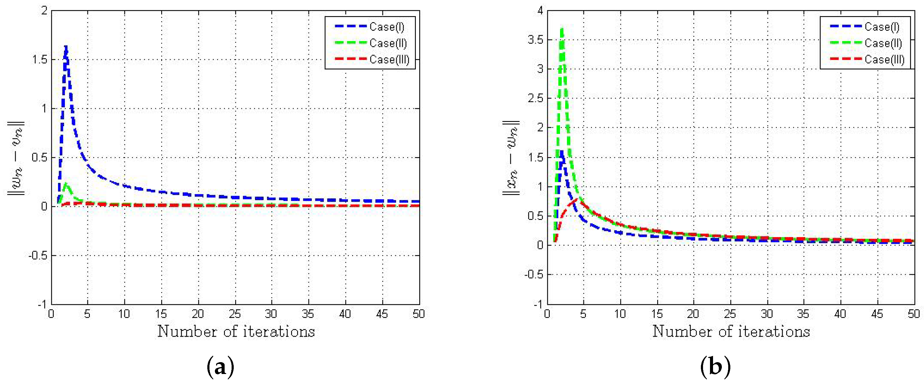
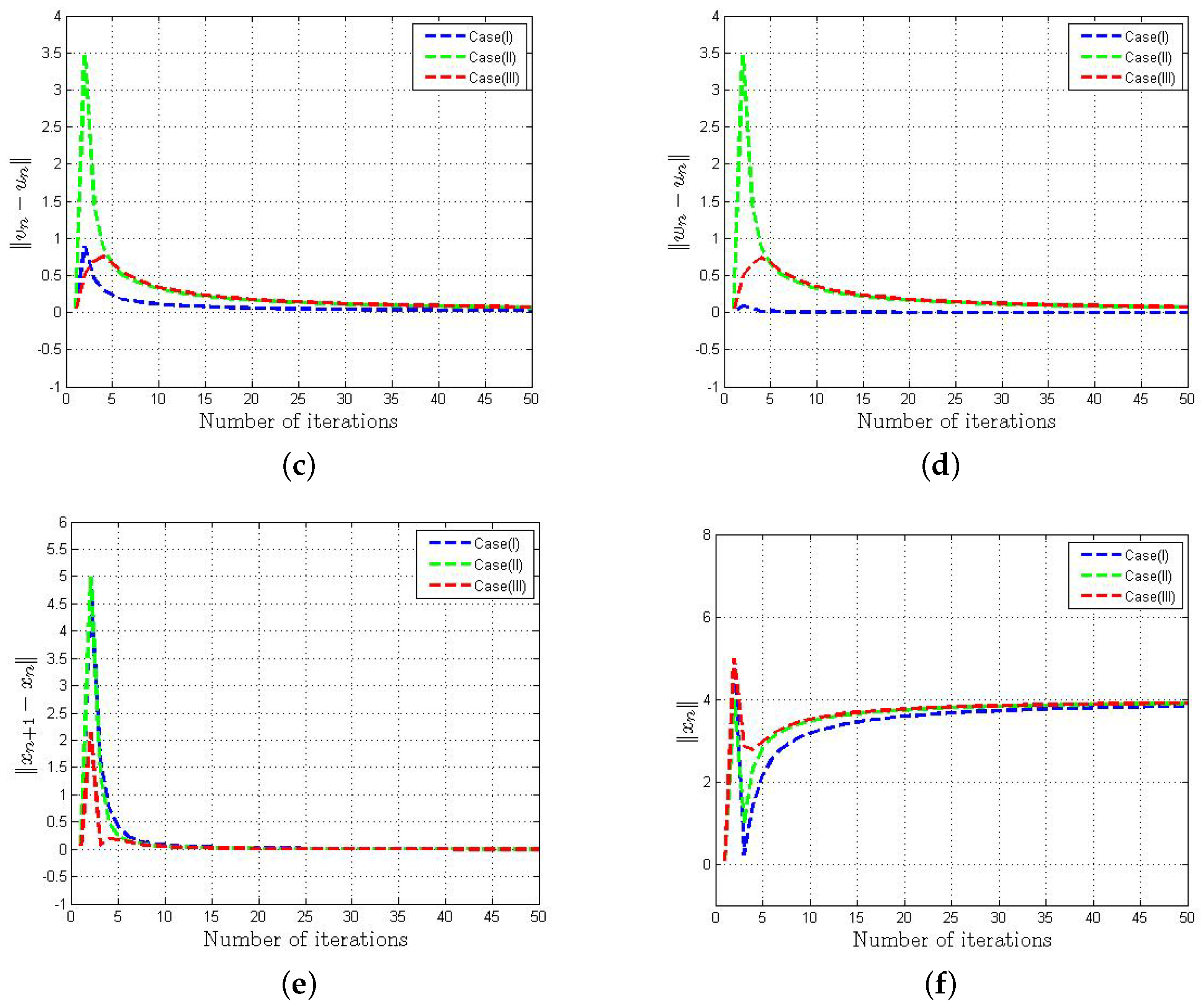
Suppose X 1 = X 2 = R . Let us consider the monotone mappings A 1 and A 2 defined as A 1 ( x ) = x 2 + 2 and A 2 ( x ) = x + 2 . The nonexpansive mapping F : X 1 X 1 is defined as F ( x ) = x 4 2 and bounded linear operator B : X 1 X 2 is defined as B ( x ) = x 2 . It is not a difficult task to show that A 1 and A 2 are monotone mappings and B is nonexpansive mapping and Fix ( F ) Λ = { 4 } . The resolvents of A 1 and A 2 with parameter μ 1 > 0 , μ 2 > 0 are
R μ 1 A 1 ( x ) = [ I + μ 1 A 1 ] 1 ( x ) = 2 x 4 μ 1 2 + μ 1 , R μ 2 A 2 ( x ) = [ I + μ 2 A 2 ] 1 ( x ) = x 2 μ 2 1 + μ 2 .
We choose τ n = 1 1 n + 1 , Λ n = 1 n 2 , ξ = 1 n and ζ n = ( 1 e 1 n 3 ) satisfying the condition (28) in Algorithm 2. We fixed the maximum number of iterations 50 as a stopping criterion. The parameter ϕ n is randomly generated in ( 0 , ϕ ˜ n ) , where ϕ ˜ n is calculated by using (14). The behavior of the sequences { x n } , { v n } and { u n } are plotted in Figure 1 by applying three distinct cases of parameters which are mentioned below:
  • Case (I): x 0 = 0 , x 1 = 5 , ϕ = 0.1 , μ 1 = 0.5 , μ 2 = 0.9 .
  • Case (II): x 0 = 3 , x 1 = 4 , ϕ = 0.5 , μ 1 = 5 , μ 2 = 8 .
  • Case (III): x 0 = 5 , x 1 = 5 , ϕ = 0.75 , μ 1 = 10 , μ 2 = 20 .
Observations:
  • In Figure 1a–d, we observed that the behavior of { w n } , { v n } and { u n } is uniform irrespective of the selection of parameters.
  • From Figure 1e–f, we notice that the sequence obtained from Algorithm 2 converges to the same limit with a suitable selection of parameters.
  • It is worthwhile to mention that the estimation of B B * is not required to implement the algorithm, which is not so handy to calculate in general.

6. Conclusions

We have suggested and analyzed inertial methods to estimate the solution of ( S p VI s P ) and common solution of ( S p VI s P ) and ( FPP ) . We proved the weak and strong convergence of algorithms to estimate the solution of ( S p VI s P ) and ( FPP ) with suitable assumptions in such a way that the estimation of the step size does not require a pre-estimated norm B B * . Finally, we perform a numerical example to exhibit the behavior of the proposed algorithms using different cases of parameters.

Author Contributions

Conceptualization, M.D.; methodology, D.F.; validation, M.A.; formal analysis, D.F.; investigation, L.S.M.A.; writing, original draft preparation, M.D.; funding acquisition, D.F.; writing, review and editing, M.A. All authors have read and agreed to the published version of the manuscript.

Funding

This research received no external funding.

Institutional Review Board Statement

Not applicable.

Informed Consent Statement

Not applicable.

Data Availability Statement

Not applicable.

Acknowledgments

The authors thank to the referees for their invaluable suggestions and comments which bring the manuscript in the current form. The researchers wish to extend their sincere gratitude to the Deanship of Scientific Research at the Islamic University of Madinah for the support provided to the Post-Publishing Program 2.

Conflicts of Interest

The authors declare no conflict of interest.

References

  1. Censor, Y.; Elfving, T. A multi projection algorithm using Bregman projections in a product space. Numer. Algor. 1994, 8, 221–239. [Google Scholar] [CrossRef]
  2. Censor, Y.; Bortfeld, T.; Martin, B.; Trofimov, A. A unified approach for inversion problem in intensity modulated radiation therapy. Phys. Med. Biol. 2006, 51, 2353–2365. [Google Scholar] [CrossRef] [PubMed]
  3. Censor, Y.; Elfving, T.; Kopf, N.; Bortfeld, T. The multiple-sets split feasibility problem and its applications for inverse problems. Inverse Probl. 2005, 21, 2071–2084. [Google Scholar] [CrossRef]
  4. Censor, Y.; Motova, X.A.; Segal, A. Perturbed projections and subgradient projections for the multiple-sets split feasibility problem. J. Math. Anal. Appl. 2007, 327, 1244–1256. [Google Scholar] [CrossRef]
  5. Masad, E.; Reich, S. A note on the multiple-set split convex feasibility problem in Hilbert space. J. Nonlinear Convex Anal. 2007, 8, 367–371. [Google Scholar]
  6. Censor, Y.; Gibali, A.; Reich, S. The split variational inequality problem, The Technion Institute of Technology, Haifa. arXiv 2010, arXiv:1009.3780. [Google Scholar]
  7. Censor, Y.; Gibali, A.; Reich, S. Algorithms for the split variational inequality problem. Numer. Alg. 2012, 59, 301–323. [Google Scholar] [CrossRef]
  8. Moudafi, A. Split monotone variational inclusions. J. Optim. Theory Appl. 2011, 150, 275–283. [Google Scholar] [CrossRef]
  9. Byrne, C.; Censor, Y.; Gibali, A.; Reich, S. Weak and strong convergence of algorithms for split common null point problem. J. Nonlinear Convex Anal. 2012, 13, 759–775. [Google Scholar]
  10. Kazmi, K.R.; Rizvi, S.H. An iterative method for split variational inclusion problem and fixed point problem for a nonexpansive mapping. Optim. Lett. 2014, 8, 1113–1124. [Google Scholar] [CrossRef]
  11. Dilshad, M.; Aljohani, A.F.; Akram, M. Iterative scheme for split variational inclusion and a fixed-point problem of a finite collection of nonexpansive mappings. J. Funct. Spaces 2020, 2020, 3567648. [Google Scholar] [CrossRef]
  12. Sitthithakerngkiet, K.; Deepho, J.; Kumam, P. A hybrid viscosity algorithm via modify the hybrid steepest descent method for solving the split variational inclusion in image reconstruction and fixed point problems. Appl. Math. Comp. 2015, 250, 986–1001. [Google Scholar] [CrossRef]
  13. Akram, M.; Dilshad, M.; Rajpoot, A.K.; Babu, F.; Ahmad, R.; Yao, J.-C. Modified iterative schemes for a fixed point problem and a split variational inclusion problem. Mathematics 2022, 10, 2098. [Google Scholar] [CrossRef]
  14. Alansari, M.; Farid, M.; Ali, R. An iterative scheme for split monotone variational inclusion, variational inequality and fixed point problems. Adv. Differ. Equ. 2020, 485, 1–21. [Google Scholar] [CrossRef]
  15. Abubakar, J.; Kumam, P.; Deepho, J. Multistep hybrid viscosity method for split monotone variational inclusion and fixed point problems in Hilbert spaces. AIMS Math. 2020, 5, 5969–5992. [Google Scholar] [CrossRef]
  16. Alansari, M.; Dilshad, M.; Akram, M. Remark on the Yosida approximation iterative technique for split monotone Yosida variational inclusions. Comp. Appl. Math. 2020, 39, 203. [Google Scholar] [CrossRef]
  17. Dilshad, M.; Siddiqi, A.H.; Ahmad, R.; Khan, F.A. An Iterative Algorithm for a Common Solution of a Split Variational Inclusion Problem and Fixed Point Problem for Non-expansive Semigroup Mappings. In Industrial Mathematics and Complex Systems; Manchanda, P., Lozi, R., Siddiqi, A., Eds.; Industrial and Applied Mathematics; Springer: Singapore, 2017. [Google Scholar]
  18. Taiwo, A.; Alakoya, T.O.; Mewomo, O.T. Halpern-type iterative process for solving split common fixed point and monotone variational inclusion problem between Banach spaces. Numer. Algor. 2021, 86, 1359–1389. [Google Scholar] [CrossRef]
  19. Zhu, L.-J.; Yao, Y. Algorithms for approximating solutions of split variational inclusion and fixed-point problems. Mathematics 2023, 11, 641. [Google Scholar] [CrossRef]
  20. Lopez, G.; Martin-Marquez, V.; Xu, H.K. Solving the split feasibilty problem without prior’ knowledge of matrix norms. Inverse Prob. 2012, 28, 085004. [Google Scholar] [CrossRef]
  21. Dilshad, M.; Akram, M.; Ahmad, I. Algorithms for split common null point problem without pre-existing estimation of operator norm. J. Math. Inequal. 2020, 14, 1151–1163. [Google Scholar] [CrossRef]
  22. Gibali, A.; Mai, D.T.; Nguyen, T.V. A new relaxed CQ algorithm for solving Split Feasibility Problems in Hilbert spaces and its applications. J. Indus. Manag. Optim. 2018, 2018, 1–25. [Google Scholar] [CrossRef]
  23. Moudafi, A.; Gibali, A. l1l2 Regularization of split feasibility problems. Numer. Algorithms 2017, 1–19. [Google Scholar] [CrossRef]
  24. Moudafi, A.; Thakur, B.S. Solving proximal split feasibilty problem without prior knowledge of matrix norms. Optim. Lett. 2014, 8, 2099–2110. [Google Scholar] [CrossRef]
  25. Shehu, Y.; Iyiola, O.S. Convergence analysis for the proximal split feasibiliy problem using an inertial extrapolation term method. J. Fixed Point Theory Appl. 2017, 19, 2483–2510. [Google Scholar] [CrossRef]
  26. Tang, Y. New algorithms for split common null point problems. Optimization 2020, 1141–1160. [Google Scholar] [CrossRef]
  27. Alvarez, F.; Attouch, H. An inertial proximal method for maximal monotone operators via discretization of a nonlinear osculattor with damping. Set-Valued Anal. 2001, 9, 3–11. [Google Scholar] [CrossRef]
  28. Tang, Y.; Zhang, Y.; Gibali, A. New self-adaptive inertial-like proximal point methods for the split common null point problem. Symmetry 2021, 13, 2316. [Google Scholar] [CrossRef]
  29. Alansari, M.; Ali, R.; Farid, M. Strong convergence of an inertial iterative algorithm for variational inequality problem, generalized equilibrium problem, and fixed point problem in a Banach space. J. Inequal. Appl. 2020, 42, 1–22. [Google Scholar] [CrossRef]
  30. Abbas, H.A.; Aremu, K.O.; Jolaoso, L.O.; Mewomo, O.T. An inertial forward-backward splitting method for approximating solutions of certain optimization problems. J. Nonlinear Func. Anal. 2020, 2020, 6. [Google Scholar]
  31. Dilshad, M.; Akram, M.; Nsiruzzaman, M.d.; Filali, D.; Khidir, A.A. Adaptive inertial Yosida approximation iterative algorithms for split variational inclusion and fixed point problems. AIMS Math. 2023, 8, 12922–12942. [Google Scholar] [CrossRef]
  32. Liu, L.; Cho, S.Y.; Yao, J.C. Convergence analysis of an inertial T-seng’s extragradient algorithm for solving pseudomonotone variational inequalities and applications. J. Nonlinear Var. Anal. 2021, 5, 627–644. [Google Scholar]
  33. Tang, Y.; Lin, H.; Gibali, A.; Cho, Y.-J. Convegence analysis and applicatons of the inertial algorithm solving inclusion problems. Appl. Numer. Math. 2022, 175, 1–17. [Google Scholar] [CrossRef]
  34. Tang, Y.; Gibali, A. New self-adaptive step size algorithms for solving split variational inclusion problems and its applications. Numer. Algor. 2019, 83, 305–331. [Google Scholar] [CrossRef]
  35. Xu, H.K. Iterative algorithms for nonlinear operators. J. Lond. Math. Soc. 2002, 66, 240–256. [Google Scholar] [CrossRef]
  36. Bauschke, H.H.; Combettes, P.L. Convex Analysis and Monotone Operator Theory in Hilbert Spaces; Springer: Berlin/Heidelberg, Germany, 2011. [Google Scholar]
  37. Opial, Z. Weak covergence of the sequence of successive approximations of nonexpansive mappings. Bull. Amer. Math. Soc. 1976, 73, 591–597. [Google Scholar] [CrossRef]
  38. Mainge, P.E. Strong convergence of projected subgradient methods for nonsmooth and nonstrictly convex minimization. Set-Valued Anal. 2008, 16, 899–912. [Google Scholar] [CrossRef]
Figure 1. Numerical behavior of w n u n , x n u n , v n u n , w n u n , x n + 1 x n and x n choosing three cases of parameters.
Axioms 12 00848 g001aAxioms 12 00848 g001b
Disclaimer/Publisher’s Note: The statements, opinions and data contained in all publications are solely those of the individual author(s) and contributor(s) and not of MDPI and/or the editor(s). MDPI and/or the editor(s) disclaim responsibility for any injury to people or property resulting from any ideas, methods, instructions or products referred to in the content.

