A Novel Robust Metric Distance Optimization-Driven Manifold Learning Framework for Semi-Supervised Pattern Classification

Abstract

In this work, we address the problem of improving the classification performance of machine learning models, especially in the presence of noisy and outlier data. To this end, we first innovatively design a generalized adaptive robust loss function called $V_{\theta }(x)$. Intuitively, $V_{\theta }(x)$ can improve the robustness of the model by selecting different robust loss functions for different learning tasks during the learning process via the adaptive parameter $\theta$. Compared with other robust loss functions, $V_{\theta }(x)$ has some desirable salient properties, such as symmetry, boundedness, robustness, nonconvexity, and adaptivity, making it suitable for a wide range of machine learning applications. Secondly, a new robust semi-supervised learning framework for pattern classification is proposed. In this learning framework, the proposed robust loss function $V_{\theta }(x)$ and capped $L_{2,p}$-norm robust distance metric are introduced to improve the robustness and generalization performance of the model, especially when the outliers are far from the normal data distributions. Simultaneously, based on this learning framework, the Welsch manifold robust twin bounded support vector machine (WMRTBSVM) and its least-squares version are developed. Finally, two effective iterative optimization algorithms are designed, their convergence is proved, and their complexity is calculated. Experimental results on several datasets with different noise settings and different evaluation criteria show that our methods have better classification performance and robustness. With the Cancer dataset, when there is no noise, the classification accuracy of our proposed methods is $94.17\%$ and $95.62\%$, respectively. When the Gaussian noise is $50\%$, the classification accuracy of our proposed methods is $91.76\%$ and $90.59\%$, respectively, demonstrating that our method has satisfactory classification performance and robustness.

1. Introduction

Data collecting and reasonable processing are becoming increasingly crucial as modern computer technology advances. As an excellent machine learning tool, support vector machine (SVM) [1,2,3] has been widely used in bioinformatics, computer vision, data mining, robotics, and other fields in recent years. The main idea behind SVM classification based on statistical learning theory and optimization theory is to construct a pair of parallel hyperplanes to maximize the minimum distance between two classes of samples. SVMs implement the structural risk minimization (SRM) principle in addition to empirical risk minimization. Although SVM can achieve good classification performance, it needs to solve a large-scale quadratic programming problem (QPP), and learning it takes a lot of time, which seriously hinders the application of SVM in large-scale classification tasks [4]. Furthermore, when dealing with complicated data, the simple SVM model would run into various issues, which will stymie its development and practical implementation, such as the “XOR” problem.

To overcome the difficulties brought by SVM to solve a QP problem, Jayadeva et al. [5] proposed a twin support vector machine (TSVM) for pattern classification based on generalized eigenvalue approximation support vector machine (GEPSVM). Since TSVM solves two smaller QPP problems instead of a single large QPP problem, it can theoretically learn four times faster than a standard SVM. The main goal of TSVM is to find two parallel hyperplanes, each of which is as close as possible to the corresponding class in the sample data, while being as far away from the other classes as possible. Further, to overcome the problem that TSVM only considers empirical risk minimization without considering the principle of structural risk minimization, Shao et al. [6] proposed a twin bounded support vector machine (TBSVM) by introducing two regularization terms. Compared with TSVM, a significant advantage of TBSVM is the principle of structural risk minimization, which embodies the essence of statistical learning theory, so this improvement can improve the classification performance of TSVM. In recent years, some TSVM-based variant algorithms have been proposed for pattern classification tasks, such as least squares twin support vector machine (LSTSVM) [4], recursive projection twin support vector machine (RPTSVM) [7], pinball twin support vector machine (Pin-TSVM) [8], sparse pinball twin support vector machine (SPTWSVM) [9], least squares recursive projection twin support vector machine (LSRPTSVM) [10], fuzzy twin support vector machine (FBTSVM) [11], and so on, which greatly promoted the development of TSVM.

It is well known that distance metrics play a crucial role in many machine learning algorithms [12]. Although the above algorithms show good performance in pattern classification, it is worth noting that most of them adopt the $L_2$-norm distance metric, whose squaring operation will exaggerate the impact of outliers on model performance. To effectively alleviate the impact of the $L_2$-norm distance metric on the robustness of the algorithm, the $L_1$-norm distance metric c with bounded derivative has received extensive attention and research in many fields of machine learning in recent years [13,14,15,16,17,18]. For example, Zhu et al. [13] proposed 1-norm SVM (1-SVM) based on an SVM learning framework. Mangasarian [14] proposed an exact $L_1$-norm support vector machine based on unconstrained convex differentiable minimization. Gao [15] developed a new 1-norm least squares TSVM (NELSTSVM). Ye et al. [16] proposed a $L_1$-norm distance minimization-based robust TSVM. Yan et al. [17] proposed 1-norm projection TSVM (1-PTSVM), and so on. As mentioned earlier, the $L_1$-norm is a better alternative to the squared $L_2$-norm in terms of enhancing the robustness of the algorithm. However, when the outliers are large, the existing classification methods based on $L_1$-norm distance often cannot achieve satisfactory classification results.

Recently, more and more researchers have paid attention to the capped $L_1$-norm and achieved some excellent research results [19,20,21,22,23,24]. Research shows that capped $L_1$-norm is considered to be a better approximation of $L_0$-norm and more robust than $L_1$-norm. In general, the capped $L_1$-norm is considered to be a better approximation of the $L_1$-norm, with stronger robustness than the $L_1$-norm. Some excellent algorithms based on capped $L_1$-norm have been proposed for robust classification tasks. For example, Wang et al. [25] proposed a new robust TSVM (CTSVM) by applying capped $L_1$-norm. CTSVM retains the advantages of TSVM and improves the robustness of classification. The experimental results on multiple datasets show that the CTSVM algorithm has good robustness and effectiveness to outliers. The capped $L_1$-norm metrics are neither convex nor smooth, which makes them difficult to optimize. There are two general strategies for solving nonconvex optimization problems. The first strategy is to design efficient algorithms, such as the bump process algorithm and the abnormal path algorithm. The second strategy is to smooth the metric function to reduce the complexity of the algorithm. To overcome the shortcomings of capped $L_1$-norm, many scholars proposed capped $L_{2,p}$-norm for robust learning [26,27]. Zhang et al. [28] proposed a new large-scale semi-supervised classification algorithm based on ridge regression and capped $L_{2,p}$-norm loss function. It is worth noting that by setting the appropriate p-value, the capped $L_1$-norm and capped $L_2$-norm are special forms of capped $L_{2,p}$-norm: when $p=1$ or $p=2$, the capped $L_{2,p}$-norm corresponds to the capped $L_1$-norm or capped $L_2$-norm. These algorithms show that the capped distance metric is robust against outliers. However, there are few extensions and related applications of the capped $L_{2,p}$-norm for twin support vector machine.

In the current scenario, although data collection is easy, obtaining labeled data is difficult [29]. To address this issue, researchers have proposed semi-supervised learning (SSL) [29], which uses less labeled data and more unlabeled data to build more reliable classifiers. Graph-based SSL algorithms are a significant branch of SSL. The learning strategy involves first forming edges by connecting points between labeled and unlabeled data points and then creating a graph from these edges that represents the similarity between samples. Manifold regularization-based SSL [30] is one of the graph-based SSL methods that preserve the manifold structure to improve the discriminative property of the data [31]. The learning strategy involves mining the geometric distribution information of the data and representing it in the form of regularization terms. The reference [31] first introduced MR to SSL by proposing the Laplace support vector machine (Lap-SVM) and Laplace regularized least squares (Lap-RLS). Qi et al. [32] developed a Laplace TSVM (LapTSVM) based on a pair of non-parallel hyperplanes of TSVM. Although the classifier’s generalization performance is improved, the method’s parameter adjustment may be impacted by different datasets, and it may not be able to handle large-scale problems effectively due to high computational complexity. Xie et al. [33] propose a novel Laplacian $L_p$-norm least squares twin support vector machine (Lap-$L_p$LSTSVM). The experimental results on both synthetic and real-world datasets show that Lap-$L_p$LSTSVM outperforms other state-of-the-art methods and can also deal with noisy datasets [34,35].

To summarize, prior research on improving the TBSVM classification performance while considering robustness and discriminability is limited. In response, we introduce the WMRTBSVM and WMLSRTBSVM models. Specifically, we replace the hinge loss term in TBSVM with the $L_{2,p}$-norm, and we replace the second term in TBSVM with the Welsch Loss with p-power. This improves the model’s classification performance and robustness. Furthermore, we incorporate a manifold structure into the model to further enhance its classification performance and discriminability. The main contributions of this paper are summarized as follows:

(1)

A generalized adaptive robust loss function called $V_{\theta }(x)$ is innovatively designed. Intuitively, $V_{\theta }(x)$ can improve the robustness of the model by selecting different robust loss functions for different learning tasks during the learning process via the adaptive parameter $\theta$. Compared with other robust loss functions, $V_{\theta }(x)$ has some desirable salient properties, such as symmetry, boundedness, robustness, nonconvexity, and adaptivity.

(2)

A novel robust manifold learning framework for semi-supervised pattern classification is proposed. In this learning framework, the proposed robust loss function $V_{\theta }(x)$ and capped $L_{2,p}$-norm robust distance metric are introduced to improve the robustness and generalization performance of the model, especially when the outliers are far from the normal data distributions.

(3)

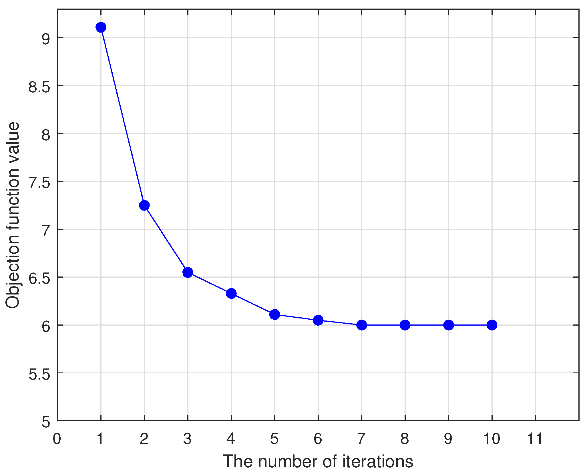
Two effective iterative optimization algorithms are designed for solving our methods by the half-quadratic (HQ) optimization algorithm, and the convergence of the algorithms is demonstrated.

(4)

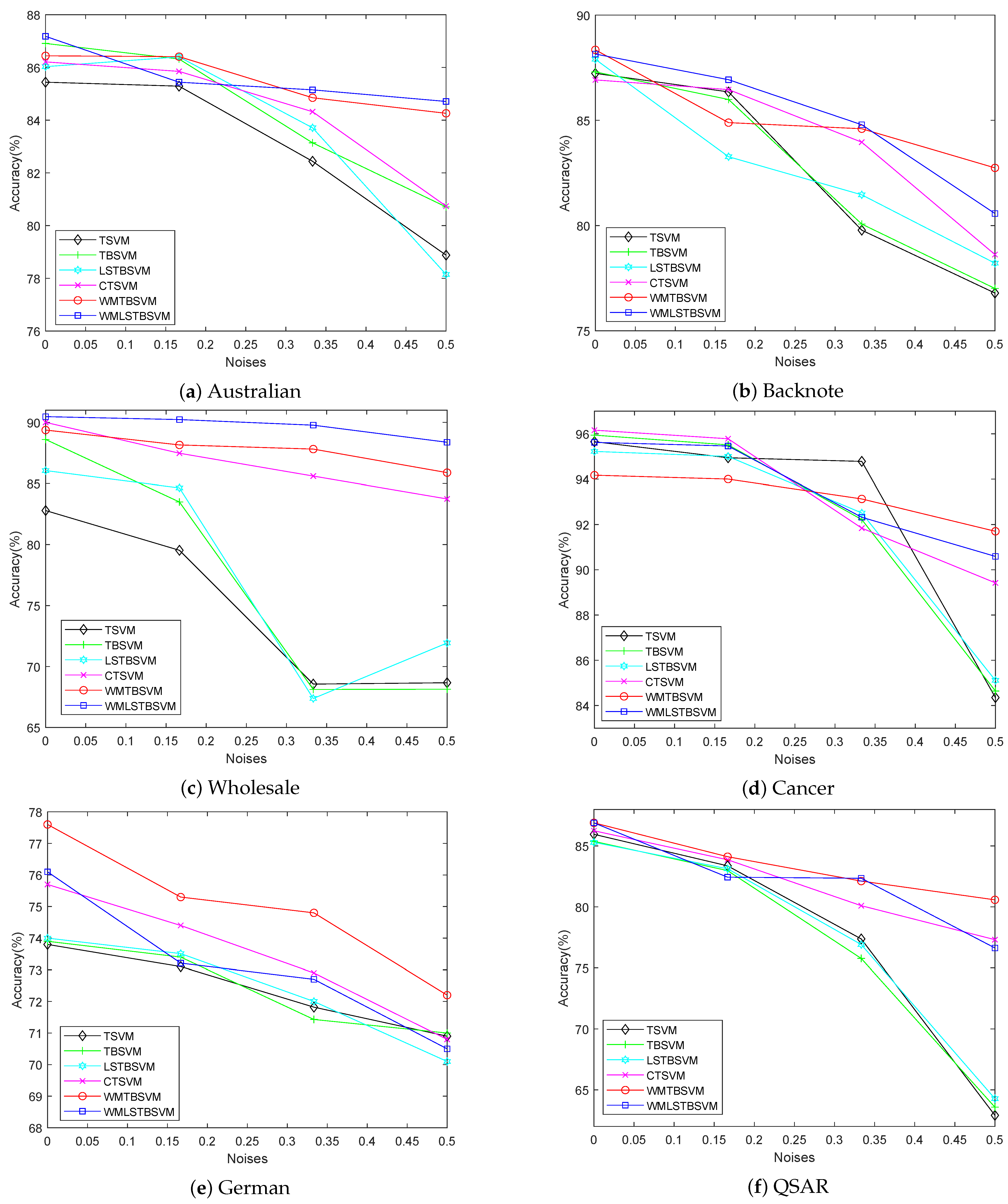
Experimental results on artificial and benchmark datasets with different noise settings and different evaluation criteria show that our methods have better classification performance and robustness.

In Section 2, we introduce the formulas involved in TBSVM and manifold regularization since our model is based on these two approaches. In Section 3, we present a novel robust manifold learning framework for semi-supervised pattern classification. Finally, we discuss experiments and conclusions in Section 4 and Section 5, respectively.

The structure of the rest of this paper is as follows: In Section 2, as our model is based on TBSVM and manifold regularization, in order to improve our formulas and their derivation, we will introduce the formulas involved in TBSVM and manifold regularization, respectively. In Section 3, we present a novel robust manifold learning framework for semi-supervised pattern classification. Finally, in Section 4 and Section 5, we discuss experiments and conclusions.

2. Related Works

This section presents a review of related works, which include TBSVM and manifold regularization. The binary classification problem in the n-dimensional real vector space ${\mathbb{R}}^n$ is considered. All vectors are represented as columns. Given a training dataset $T=(x_1,y_1),\dots ,(x_m,y_m)$, where $x_i\in {\mathbb{R}}^n$ is the input and $y_i=\{-1,1\}$ is the corresponding output for $i=1,\dots ,m$. T is composed of $m_1$ positive class and $m_2$ negative class samples, where m = $m_1$ + $m_2$. The data samples from class i form the data matrix $X_i\in {\mathbb{R}}^{n\times n}$, where each column represents a sample. $A\in {\mathbb{R}}^{n\times m_1}$ represents all positive class samples (i.e., $y_i=1$), and $B\in {\mathbb{R}}^{n\times m_2}$ represents all negative classes (i.e., $y_i=-1$).

2.1. TBSVM

In this subsection, we provide a brief review of the twin bounded support vector machine (TBSVM). The optimization objective of TBSVM is to ensure that each hyperplane is as close as possible to the samples in the corresponding class and as far away as possible from the samples in the other class. For the linear case, TBSVM defines two nonparallel hyperplanes:

$$\begin{array}{c}\hfill f_1(x)={\omega }_1^{T}x+b_1=0and{f}_2(x)={\omega }_2^{T}x+b_2=0.\end{array}$$

(1)

To improve the classification ability of TSVM and realize the principle of structural risk minimization, an improved version of TSVM named TBSVM is obtained by introducing an $L_2$-regularization term based on TSVM:

$$\begin{array}{cc}\hfill & \underset{{\omega }_1,b_1,{\xi }_1}{min}\frac{1}{2}\parallel A{\omega }_1+e_1{b}_1{\parallel }_2^2+c_1{e}_2^T{\xi }_1+\frac{c_3}{2}(\parallel {\omega }_1{\parallel }_2^2+b_1^2)\hfill \\ \hfill & s.t.-(B{\omega }_1+e_2{b}_1)+{\xi }_1\ge e_2,{\xi }_1\ge 0,\hfill \end{array}$$

(2)

and

$$\begin{array}{cc}\hfill & \underset{{\omega }_2,b_2,{\xi }_2}{min}\frac{1}{2}\parallel B{\omega }_2+e_2{b}_2{\parallel }_2^2+c_2{e}_1^T{\xi }_2+\frac{c_4}{2}(\parallel {\omega }_2{\parallel }_2^2+b_2^2),\hfill \\ \hfill & s.t.(A{\omega }_2+e_1{b}_2)+{\xi }_2\ge e_1,{\xi }_2\ge 0.\hfill \end{array}$$

(3)

To avoid the impact of singular problems caused by inverse matrices, positive scales ${\lambda }_{1}I$ and ${\lambda }_{2}I$ are introduced, where ${\lambda }_1$ and ${\lambda }_2$ are small positive constants, and 0 and I represent the zero vector matrix and the identity matrix, respectively, on the appropriate dimension. Therefore, based on the dual theory, we can obtain the dual problem of (2) and (3):

$$\begin{array}{cc}\hfill & \underset{\alpha }{min}\frac{1}{2}{\alpha }^{T}G{(H^{T}H+c_{3}I)}^{-1}{G}^T\alpha -e_2^T\alpha \hfill \\ \hfill & s.t.0\le \alpha \le c_1{e}_2,\hfill \end{array}$$

(4)

and

$$\begin{array}{cc}\hfill & \underset{\beta }{min}\frac{1}{2}{\beta }^{T}H{(G^{T}G+c_{4}I)}^{-1}{H}^T\beta -e_1^T\beta ,\hfill \\ \hfill & s.t.0\le \beta \le c_2{e}_1.\hfill \end{array}$$

(5)

where $c_1,c_2,c_3,c_4>0$ represent regularization parameters, $e_1\in {\mathbb{R}}^{m_1}$ and $e_2\in {\mathbb{R}}^{m_2}$ are vectors of ones, and ${\xi }_1$ and ${\xi }_2$ are slack vectors. The prime superscript T is used to transform column vectors into row vectors, and the matrices $G=[B{e}_2]$ and $H=[A{e}_1]$. The dual problems are revised as $\alpha \in {\mathbb{R}}^{m_2}$ and $\beta \in {\mathbb{R}}^{m_1}$, which are Lagrange multipliers. By solving (4) and (5), two nonparallel hyperplanes can be obtained:

$$\begin{array}{c}\hfill \left[\begin{array}{c}{\omega }_1\\ b_1\end{array}\right]=-{(H^{T}H+c_{3}I)}^{-1}{G}^T\alpha and\left[\begin{array}{c}{\omega }_2\\ b_2\end{array}\right]={(G^{T}G+c_{4}I)}^{-1}{H}^T\beta .\end{array}$$

A new data point $x\in {\mathbb{R}}^n$ is then assigned to the positive or negative class, depending on which of the two hyperplanes (1) it lies closest to, i.e.,

$$f(x)=argmi{n}_{k=1,2}\frac{|x{\omega }_k+b_k|}{\parallel {\omega }_k\parallel },$$

where $|.|$ is the absolute value operation, ${\parallel .\parallel }_p$ means the $L_p$-norm for $p>0$, when $p=2$, ${\parallel .\parallel }_2$ is written as $\parallel .\parallel$ for brevity.

2.2. Manifold Regularization

In this subsection, we briefly review graph-based semi-supervised learning (SSL). Manifold regularization (MR) is one of the graph-based SSL methods, whose learning strategy is to mine the geometric distribution information of the data and represent it in the form of regularization terms. In [30], the authors point out that data distributions on manifolds are often complex and may exhibit nonlinear structures, and traditional methods may not be able to effectively capture their intrinsic structures and characteristics. Based on this, the authors propose a regularization method based on the Laplacian graph. On the basis of ensuring smoothness, the method maintains the Euclidean distance relationship of the original data sample as far as possible, enabling it to better reflect the distribution of data in the manifold space.

Consider a binary semi-supervised classification problem in the n-dimensional real space ${\mathbb{R}}^n$. The set of training data is represented by $\mathcal{T}=\{(x_1,y_1),\dots ,(x_l,y_l),x_{l+1},\dots ,x_{l+u}\}$, where $l+u=n$, dataset ${\mathcal{X}}_l={\left\{x_i\right\}}_{i=1}^l\in {\mathbb{R}}^{l\times n}$ are the labeled data with corresponding labels ${\mathcal{Y}}_l={\left\{y_i\right\}}_{i=1}^l\in \{-1,1\}$, and dateset ${\mathcal{X}}_u={\left\{x_i\right\}}_{i=1}^u\in {\mathbb{R}}^{u\times n}$ are the unlabeled data with corresponding labels ${\mathcal{Y}}_u=0$, where $\mathcal{X}={\mathcal{X}}_l+{\mathcal{X}}_u$ represent the whole dateset. We model $\mathcal{X}$ as a graph $\mathcal{G}$, $\mathbf{W}$ is the adjacency matrix of graph $\mathcal{G}$,

$$\begin{array}{c}\hfill w_{ij}:=\left\{\begin{array}{cc}& exp(\frac{-\parallel x_i-x_j{\parallel }^2}{2{\sigma }^2}),x_i\in N_k(x_j)or{x}_j\in N_k(x_i),\hfill \\ & 0,Otherwise,\hfill \end{array}\right.\end{array}$$

denotes the similarity between examples $x_i$ and $x_j$, where $N_k(x_j)$ represents the k nearest neighbors of $x_i$. Based on the adjacency matrix $\mathbf{W}$, the Laplacian matrix $\mathbf{L}$ of the graph $\mathcal{X}$ can be computed by $\mathbf{L}=\mathbf{D}-\mathbf{W}$, where $\mathbf{D}=diag({\sum }_{j=1}^n{W}_{1j},{\sum }_{j=1}^n{W}_{2j},\dots ,{\sum }_{j=1}^n{W}_{nj})$.

In RKHS, the optimization of manifold regularization can be written as follows:

$$\begin{array}{c}\hfill f^{*}=arg\underset{f\in H}{min}{R}^{emp}(f)+{\gamma }_H{\parallel f\parallel }_H^2+{\gamma }_M{\parallel f\parallel }_M^2,\end{array}$$

where $R^{emp}(f)$ denotes the empirical risks on the labeled data $\mathcal{Y}$, which also denote the loss function. ${\gamma }_H$ and ${\gamma }_M$ are non-negative regularization parameters. ${f\parallel }_H^2$ is the regularization term to prevent overfitting. ${f\parallel }_M^2$ is the smoothness term, which can be expressed as:

$$\begin{array}{c}\hfill {\parallel f\parallel }_M^2=\frac{1}{{(l+u)}^2}\sum _{i,j=1}^{l+u}{w}_{ij}{(f(x_i)-f(x_j))}^2=f^{T}Lf.\end{array}$$

(6)

3. Main Contributions

In this section, we begin by outlining the key motivation behind our proposed model. We then present the model formulation and describe its components in detail. Finally, we provide a convergence analysis of the proposed model in Section 3.3.

3.1. Generalized Adaptive Robust Loss Function

To improve the robustness, classification performance, and generalization ability of the TBSVM framework, we propose a new robust loss function called the generalized adaptive robust loss function $V_{\theta }(x)$. The $V_{\theta }(x)$ loss function is symmetric and has bounded non-negativity. The $V_{\theta }(x)$ is defined for any $x\in R^n$ as follows:

$$\begin{array}{c}\hfill V_{\theta }(x)=\frac{c^2}{2}[1-exp(-\frac{x^2}{2c^2}){]}^{\theta },\end{array}$$

(7)

where $\theta >0$ is the power parameter, and c is a trade-off parameter that penalizes outliers.

Remark 1.

When $\theta =1$, the $V_{\theta }(x)$-Loss will degenerate into Welsch Loss [36]. That is, Welsch Loss is a special case of $V_{\theta }(x)$-Loss.

Property 1.

$V_{\theta }(x)$ has boundedness, non-negativity, symmetry, lack of smoothness, and non-convexity. Secondly, its value is limited to a constant and does not increase, which ensures better robustness and desirability of the loss function.

In Figure 1, we compare the robustness of different loss functions, namely $L_2$-loss, $L_1$-loss, Welsch loss, and $V_{\theta }(x)-loss$ ($c=1$), against outliers. As shown in the figure, the Welsch Loss with $\theta$-power (red curves) is the most robust, highlighting its effectiveness in suppressing the impact of noisy outliers on the model performance. In Figure 2, we plot the loss curve of the Welsch Loss with $\theta$-power under different values of the parameter $\theta$. We observe that as $\theta$ decreases (from 4 to 2, 1, and $0.5$), the function becomes narrower while remaining symmetric and bounded, further demonstrating its suitability for handling noise and outliers.

3.2. Our Method

In this subsection, we present our model and provide an explanation of it. For the binary classification task, we aim to find a pair of optimal classification hyperplanes to separate the positive and negative samples. Specifically, we consider a pair of constrained optimization problems:

$$\begin{array}{cc}\hfill & \underset{{\omega }_1,b_1,{\xi }_1}{min}\sum _{i=1}^{m_1}min(\parallel {\omega }_1{x}_i+b_1{\parallel }_2^p,{\epsilon }_1)+c_1\sum _{i=1}^{m_2}[1-exp(-\frac{{\xi }_{1,i}^2}{2c^2}){]}^{\theta }+\frac{c_3}{2}(\parallel {\omega }_1{\parallel }_2^2+b_1^2)+c_5{f}_1^{T}L{f}_1\hfill \\ \hfill & s.t.-(B{\omega }_1+e_2{b}_1)+{\xi }_1\ge e_2,{\xi }_1\ge 0,\hfill \end{array}$$

(8)

and

$$\begin{array}{cc}\hfill & \underset{{\omega }_2,b_2,{\xi }_2}{min}\sum _{i=1}^{m_2}min(\parallel {\omega }_2{x}_i+b_2{\parallel }_2^p,{\epsilon }_3)+c_2\sum _{i=1}^{m_2}[1-exp(-\frac{{\xi }_{2,i}^2}{2c^2}){]}^{\theta }+\frac{c_4}{2}(\parallel {\omega }_2{\parallel }_2^2+b_2^2)+c_6{f}_2^{T}L{f}_2\hfill \\ \hfill & s.t.(A{\omega }_1+e_1{b}_2)+{\xi }_2\ge e_1,{\xi }_2\ge 0.\hfill \end{array}$$

(9)

where, $c_1,c_2,c_3,c_4,c_5$, and $c_6$ are positive regularization parameters, while c is an adjustment parameter that controls the degree of penalty for outliers. As stated in (6):

$$\begin{array}{c}\hfill \parallel f_1{\parallel }_M^2=\frac{1}{{(l+u)}^2}\sum _{i,j=1}^{l+u}{W}_{ij}{(f_1(x_i)-f_1(x_j))}^2=f_1^{T}L{f}_1\end{array}$$

and

$$\begin{array}{c}\hfill \parallel f_2{\parallel }_M^2=\frac{1}{{(l+u)}^2}\sum _{i,j=1}^{l+u}{W}_{ij}{(f_2(x_i)-f_2(x_j))}^2=f_2^{T}L{f}_2.\end{array}$$

where $L=D-W$ refers to the Graph Laplacian matrix. D is a diagonal matrix associated with W, where the diagonal element is $D_{ij}={\sum }_{i,j=1}^{l+u}{W}_{ij}$. The vector $f_1=[f_1{(x_1,\dots ,f_1(x_{l+u})]}^T$ equals $M{\omega }_1+e{b}_1$, while $f_2=[f_2{(x_1,\dots ,f_2(x_{l+u})]}^T$ equals $M{\omega }_2+e{b}_2$, where $M\in {\mathbb{R}}^{(l+u)\times n}$ represents all training data, including labeled and unlabeled data and e is an appropriate vector. Thus, the primary problem of (8) and (9) can be written as:

$$\begin{array}{cc}\hfill & \underset{{\omega }_1,b_1,{\xi }_1}{min}\sum _{i=1}^{m_1}min(\parallel {\omega }_1{x}_i+b_1{\parallel }_2^p,{\epsilon }_1)+c_1\sum _{i=1}^{m_1}[1-exp(-\frac{{\xi }_{1,i}^2}{2c^2}){]}^{\theta }+\frac{c_3}{2}(\parallel {\omega }_1{\parallel }_2^2+b_1^2)+c_5({\omega }_1^T{M}^T+e^T{b}_1)L({\omega }_{1}M+e{b}_1)\hfill \\ \hfill & s.t.-(B{\omega }_1+e_2{b}_1)+{\xi }_1\ge e_2,{\xi }_1\ge 0,\hfill \end{array}$$

(10)

and

$$\begin{array}{cc}\hfill & \underset{{\omega }_2,b_2,{\xi }_2}{min}\sum _{i=1}^{m_2}min(\parallel {\omega }_2{x}_i+b_2{\parallel }_2^p,{\epsilon }_3)+c_2\sum _{i=1}^{m_2}[1-exp(-\frac{{\xi }_{2,i}^2}{2c^2}){]}^{\theta }+\frac{c_4}{2}(\parallel {\omega }_2{\parallel }_2^2+b_2^2)+c_6({\omega }_2^T{M}^T+e^T{b}_2)L({\omega }_{2}M+e{b}_2)\hfill \\ \hfill & s.t.(A{\omega }_1+e_1{b}_2)+{\xi }_2\ge e_1,{\xi }_2\ge 0.\hfill \end{array}$$

(11)

Since the two terms are quite similar, we can solve one of them and obtain a solution for the other in a similar manner. For the purpose of illustration, let us consider solving (10) in two parts:

$$\left\{\begin{array}{c}P({\omega }_1,b_1)=\underset{{\omega }_1,b_1,{\xi }_1}{min}\sum _{i=1}^{m_1}min(\parallel {\omega }_1{x}_i+b_1{\parallel }_2^p,{\epsilon }_1)+\frac{c_3}{2}(\parallel {\omega }_1{\parallel }_2^2+b_1^2)+c_5({\omega }_1^T{M}^T+e^T{b}_1)L({\omega }_{1}M+e{b}_1)\hfill \\ R({\omega }_1,b_1)=c_1\sum _{i=1}^{m_2}[1-exp(-\frac{{\xi }_1^2{,}_i}{2c^2}){]}^{\theta }\hfill \end{array}\right.$$

(12)

Then, we can rewrite the Formula (10) as:

$$\begin{array}{cc}\hfill & \underset{{\omega }_1,b_1,{\xi }_1}{max}M({\omega }_1,b_1,{\xi }_1)=\overline{R}({\omega }_1,b_1)-P({\omega }_1,b_1),\hfill \end{array}$$

(13)

where $\overline{R}({\omega }_1,b_1)=c_1{\sum }_{i=1}^{m_2}[exp(-\frac{{\xi }_{1,i}^2}{2c^2}){]}^{\theta }$. We define a convex function

$$\begin{array}{c}\hfill g(v)=-vlog(-v)+v,v<0.\end{array}$$

(14)

From the theory of conjugate functions, we obtain:

$$\begin{array}{c}\hfill exp(-\frac{{\xi }_1^2}{2c^2}{)}^{\theta }=\underset{v<0}{sup}[v\frac{{\xi }_1^2}{2c^2}-g(v){]}^{\theta },v=-exp(-\frac{{\xi }_1^2}{2c^2}{)}^{\theta }.\end{array}$$

(15)

Then, we obtain:

$$\begin{array}{cc}\hfill & \underset{{\omega }_1,b_1,{\xi }_1}{max}M({\omega }_1,b_1,{\xi }_1)=\sum _{i=1}^{m_2}([v_i\frac{{\xi }_{1,i}^2}{2c^2}-g(v_i)]{)}^{\theta }-P({\omega }_1,b_1).\hfill \end{array}$$

(16)

Thus, the (10) and (11) can be rewritten as:

$$\begin{array}{cc}\hfill & \underset{{\omega }_1,b_1,{\xi }_1}{min}\sum _{i=1}^{m_1}min(\parallel {\omega }_1{x}_i+b_1{\parallel }_2^p,{\epsilon }_1)+\frac{c_1}{2c^2}{\xi }_1^T{\mathsf{\Omega }}_1{\xi }_1+\frac{c_3}{2}(\parallel {\omega }_1{\parallel }_2^2+b_1^2)+c_5({\omega }_1^T{M}^T+e^T{b}_1)L({\omega }_{1}M+e{b}_1)\hfill \\ \hfill & s.t.-(B{\omega }_1+e_2{b}_1)+{\xi }_1\ge e_2,{\xi }_1\ge 0,\hfill \end{array}$$

(17)

and

$$\begin{array}{cc}\hfill & \underset{{\omega }_2,b_2,{\xi }_2}{min}\sum _{i=1}^{m_2}min(\parallel {\omega }_2{x}_i+b_2{\parallel }_2^p,{\epsilon }_2)+\frac{c_1}{2c^2}{\xi }_1^T{\mathsf{\Omega }}_2{\xi }_1+\frac{c_4}{2}(\parallel {\omega }_2{\parallel }_2^2+b_2^2)+c_6({\omega }_2^T{M}^T+e^T{b}_2)L({\omega }_{2}M+e{b}_2)\hfill \\ \hfill & s.t.(A{\omega }_2+e_1{b}_2)+{\xi }_2\ge e_1,{\xi }_2\ge 0,\hfill \end{array}$$

(18)

where ${\mathsf{\Omega }}_j=diag(-v_{j,i}^s,0)$, $j=1,2$. To optimize the objective function smoothly, we introduce concave duality, as illustrated in Lemma 1 [37,38].

Lemma 1.

Let $g(\theta ):R^n\to R$ be a continuous nonconvex function, suppose $h(\theta ):{\mathbb{R}}^n\to \Xi$ is a map with range Ξ. We assume that a concave function $\overline{g}(u)$ exists defined on Ξ, such that $g(\theta )=g(h(\theta ))$ holds.

Therefore, the nonconvex function $g(\theta )$ can be expressed as:

$$g(\theta )=\underset{v\in R^n}{inf}[v^{T}h(\theta )-g^{*(v)}].$$

(19)

According to concave duality, $g^{*}(v)$ is the concave dual of $\overline{g}(u)$ given as:

$$g^{*}(v)=\underset{u\in }{inf}[v^{T}h(\theta )-g^{*(v)}].$$

(20)

In addition, the minimum value to the right is as follows:

$$v^{*}=\frac{\partial \overline{g}(\theta )}{\partial \theta }{|}_{u=h(\theta )}.$$

(21)

Based on the Lemma 1, we give a non-convex function $\overline{g}(\theta ):\mathbb{R}\to \mathbb{R}$ make any arbitrary $\theta >0$,

$$\begin{array}{c}\hfill \overline{g}(\theta )=min({\theta }^{\frac{p}{2}},\epsilon ).\end{array}$$

(22)

Assuming that $h(\mu )={\mu }^2$, we obtain

$$\begin{array}{c}\hfill min(\parallel \omega x_i{+b\parallel }_2^p,\epsilon )=g(h(\mu )),\mu =\parallel \omega x_i{+b\parallel }_2\end{array}$$

(23)

Based on (23), the first term of (17) and (18) can be rewritten as:

$$\begin{array}{cc}\hfill & \underset{{\omega }_1,b_1,{\xi }_1}{min}\sum _{i=1}^{m_1}\overline{g}(\parallel {\omega }_1{x}_i+b_1{\parallel }_2^2)+\frac{c_1}{2c^2}{\xi }_1^T{\mathsf{\Omega }}_1{\xi }_1+\frac{c_3}{2}(\parallel {\omega }_1{\parallel }_2^2+b_1^2)+c_5({\omega }_1^T{M}^T+e^T{b}_1)L({\omega }_{1}M+e{b}_1)\hfill \\ \hfill & s.t.-(B{\omega }_1+e_2{b}_1)+{\xi }_1\ge e_2,{\xi }_1\ge 0,\hfill \end{array}$$

(24)

and

$$\begin{array}{cc}\hfill & \underset{{\omega }_2,b_2,{\xi }_2}{min}\sum _{i=1}^{m_2}\overline{g}(\parallel {\omega }_2{x}_i+b_2{\parallel }_2^2)+\frac{c_2}{2c^2}{\xi }_2^T{\mathsf{\Omega }}_2{\xi }_2+\frac{c_4}{2}(\parallel {\omega }_2{\parallel }_2^2+b_2^2)+c_6({\omega }_2^T{M}^T+e^T{b}_2)L({\omega }_{2}M+e{b}_2)\hfill \\ \hfill & s.t.(A{\omega }_1+e_1{b}_2)+{\xi }_2\ge e_1,{\xi }_2\ge 0.\hfill \end{array}$$

(25)

Let ${\theta }_1=h({\mu }_1)={\parallel {\omega }_1{x}_i+b_1\parallel }_2^2$. By Formula (19), the first term of (17) can be expressed as:

$$min(\parallel {\omega }_1{x}_i+b_1{\parallel }_2^p,{\epsilon }_1)=\overline{g}(\parallel {\omega }_1{x}_i+b_1{\parallel }_2^2)=\underset{f_{ii}\ge 0}{inf}(f_{ii}h({\mu }_1)-g^{*}(f_{ii}))=\underset{f_{ii}\ge 0}{inf}{f}_{ii}{\theta }_1-g^{*}(f_{ii}).$$

(26)

Therefore, the nonconvex dual function of $\overline{g}({\theta }_1)$ given as:

$$g^{*}(f_{ii})=\underset{{\theta }_1}{inf}[f_{ii}{\theta }_1-\overline{g}({\theta }_1]=\underset{{\theta }_1}{inf}\left\{\begin{array}{c}{f}_{ii}{\theta }_1-{\theta }_1^{\frac{p}{2}},{\theta }_1^{\frac{p}{2}}<{\epsilon }_1,\hfill \\ f_{ii}{\theta }_1-{\epsilon }_1,{\theta }_1^{\frac{p}{2}}\ge {\epsilon }_1.\hfill \end{array}\right.$$

(27)

By optimizing ${\theta }_1$ for (27):

$$g^{*}(f_{ii})=\left\{\begin{array}{c}{f}_{ii}{(\frac{2}{p}{f}_{ii})}^{\frac{2}{p-2}}-{(\frac{2}{p}{f}_{ii})}^{\frac{2}{p-2}},{\theta }_1^{\frac{p}{2}}<{\epsilon }_1,\hfill \\ f_{ii}{\epsilon }_1^{\frac{2}{p}}-{\epsilon }_1,{\theta }_1^{\frac{p}{2}}\ge {\epsilon }_1.\hfill \end{array}\right.$$

(28)

Finally, the objective function (17) first term can be further written as:

$$min(\parallel {\omega }_1{x}_i+b_1{\parallel }_2^p,{\epsilon }_1)=\underset{f_{ii}\ge 0}{inf}{L}_i({\omega }_1,b_1,f_{ii},{\epsilon }_1),$$

where

$$L_i({\omega }_1,b_1,f_{ii},{\epsilon }_1)\left\{\begin{array}{c}{f}_{ii}{\theta }_1-f_{ii}{(\frac{2}{p}{f}_{ii})}^{\frac{2}{p-2}}+{(\frac{2}{p}{f}_{ii})}^{\frac{2}{p-2}},{\theta }_1^{\frac{p}{2}}<{\epsilon }_1,\hfill \\ f_{ii}{\theta }_1-f_{ii}{\epsilon }_1^{\frac{2}{p}}+{\epsilon }_1,{\theta }_1^{\frac{p}{2}}\ge {\epsilon }_1.\hfill \end{array}\right.$$

(29)

Therefore, Formula (17) can be rewritten as:

$$\begin{array}{c}{\displaystyle \underset{{\omega }_1,b_1}{min}}{\displaystyle \sum _{i=1}^{m_1}}min(\parallel {\omega }_1{x}_i+b_1{\parallel }_2^p,{\epsilon }_1)+\frac{c_1}{2c^2}{\xi }_1^T{\mathsf{\Omega }}_1{\xi }_1+\frac{c_3}{2}(\parallel {\omega }_1{\parallel }_2^2+b_1^2)+c_5({\omega }_1^T{M}^T+e^T{b}_1)L({\omega }_{1}M+e{b}_1)\\ ⟺\\ {\displaystyle \underset{{\omega }_1,b_1}{min}}{\displaystyle \sum _{i=1}^{m_1}}{\displaystyle \underset{f_{ii}\ge 0}{inf}}{L}_i({\omega }_1,b_1,f_{ii},{\epsilon }_1)+\frac{c_1}{2c^2}{\xi }_1^T{\mathsf{\Omega }}_1{\xi }_1+\frac{c_3}{2}(\parallel {\omega }_1{\parallel }_2^2+b_1^2)+c_5({\omega }_1^T{M}^T+e^T{b}_1)L({\omega }_{1}M+e{b}_1)\\ ⟺\\ {\displaystyle \underset{{\omega }_1,b_1,f_{ii}\ge 0}{min}}{\displaystyle \sum _{i=1}^{m_1}}{L}_i({\omega }_1,b_1,f_{ii},{\epsilon }_1)+\frac{c_1}{2c^2}{\xi }_1^T{\mathsf{\Omega }}_1{\xi }_1+\frac{c_3}{2}(\parallel {\omega }_1{\parallel }_2^2+b_1^2)+c_5({\omega }_1^T{M}^T+e^T{b}_1)L({\omega }_{1}M+e{b}_1).\end{array}$$

(30)

Similarly, Formula (18) can be rewritten as:

$$\begin{array}{c}{\displaystyle \underset{{\omega }_2,b_2}{min}}{\displaystyle \sum _{i=1}^{m_2}}min(\parallel {\omega }_2{x}_i+b_2{\parallel }_2^p,{\epsilon }_2)+\frac{c_2}{2c^2}{\xi }_2^T{\mathsf{\Omega }}_2{\xi }_2+\frac{c_4}{2}(\parallel {\omega }_2{\parallel }_2^2+b_2^2)+c_6({\omega }_2^T{M}^T+e^T{b}_2)L({\omega }_{2}M+e{b}_2)\\ ⟺\\ {\displaystyle \underset{{\omega }_2,b_2}{min}}{\displaystyle \sum _{i=1}^{m_2}}{\displaystyle \underset{d_{ii}\ge 0}{inf}}{L}_i({\omega }_2,b_2,d_{ii},{\epsilon }_2)+\frac{c_2}{2c^2}{\xi }_2^T{\mathsf{\Omega }}_2{\xi }_2+\frac{c_4}{2}(\parallel {\omega }_2{\parallel }_2^2+b_2^2)+c_6({\omega }_2^T{M}^T+e^T{b}_2)L({\omega }_{2}M+e{b}_2)\\ ⟺\\ {\displaystyle \underset{{\omega }_2,b_2,d_{ii}\ge 0}{min}}{\displaystyle \sum _{i=1}^{m_2}}{L}_i({\omega }_2,b_2,d_{ii},{\epsilon }_2)+\frac{c_2}{2c^2}{\xi }_2^T{\mathsf{\Omega }}_2{\xi }_2+\frac{c_4}{2}(\parallel {\omega }_2{\parallel }_2^2+b_2^2)+c_6({\omega }_2^T{M}^T+e^T{b}_2)L({\omega }_{2}M+e{b}_2).\end{array}$$

(31)

The objective functions (30) and (31) are solved by learning optimal classifiers through alternative optimization algorithms. We calculate the gradient of the function $g(\theta )$ with respect to $\theta$, expressed as:

$$\frac{\partial \overline{g}(\theta )}{\partial \theta }=\left\{\begin{array}{c}\frac{p}{2}{\theta }^{\frac{p}{2}-1},0<\theta <{\epsilon }^{\frac{2}{p}},\hfill \\ 0,\theta >{\epsilon }^{\frac{2}{p}}.\hfill \end{array}\right.$$

(32)

If ${\theta }_1=h({\mu }_1)={\parallel {\omega }_1{x}_i+b_1\parallel }_2^2$, we fix ${\omega }_1$ and $b_1$:

$$f_{ii}=\frac{\partial \overline{g}({\theta }_1)}{\partial {\theta }_1}{|}_{{\theta }_1}={\parallel {\omega }_1{x}_i+b_1\parallel }_2^2=\left\{\begin{array}{c}\frac{p}{2}\parallel {\omega }_1{x}_i+b_1{\parallel }_2^{p-2},0<{\parallel {\omega }_1{x}_i+b_1\parallel }_2^p<{\epsilon }_1,\hfill \\ 0,else.\hfill \end{array}\right.$$

(33)

Similarly, if ${\theta }_2=h({\mu }_2)={\parallel {\omega }_2{x}_i+b_2\parallel }_2^2$, we fix ${\omega }_2$ and $b_2$:

$$d_{ii}=\frac{\partial \overline{g}({\theta }_2)}{\partial {\theta }_2}{|}_{{\theta }_2}={\parallel {\omega }_2{x}_i+b_2\parallel }_2^2=\left\{\begin{array}{c}\frac{p}{2}\parallel {\omega }_2{x}_i+b_2{\parallel }_2^{p-2},0<{\parallel {\omega }_2{x}_i+b_2\parallel }_2^p<{\epsilon }_3,\hfill \\ 0,else.\hfill \end{array}\right.$$

(34)

To understand the relationship between parameters more clearly, we set the distance from sample $x_i$ to the hyperplane as X. If $X>{\epsilon }_1$ and $f_{ii}$ almost equals 0, then the sample $x_i$ is considered an outlier and is discarded. Furthermore, $d_{ii}$ is similar to $f_{ii}$. When the variables $f_{ii}$ and $d_{ii}$ are fixed to solve the classifier-related parameters ${\omega }_1$, ${\omega }_2$, $b_1$, and $b_2$, the optimization problem (30) and (31) can be written as:

$$\underset{{\omega }_1,b_1}{min}\sum _{i=1}^{m_1}{f}_{ii}(\parallel {\omega }_1{x}_i+b_1{\parallel }_2^2)+\frac{c_1}{2c^2}{\xi }_1^T{\mathsf{\Omega }}_1{\xi }_1+\frac{c_3}{2}(\parallel {\omega }_1{\parallel }_2^2+b_1^2)+c_5({\omega }_1^T{M}^T+e^T{b}_1)L({\omega }_{1}M+e{b}_1)$$

(35)

and

$$\underset{{\omega }_2,b_2}{min}\sum _{i=1}^{m_2}{d}_{ii}(\parallel {\omega }_2{x}_i+b_2{\parallel }_2^2)+\frac{c_2}{2c^2}{\xi }_2^T{\mathsf{\Omega }}_2{\xi }_2+\frac{c_4}{2}(\parallel {\omega }_2{\parallel }_2^2+b_2^2)+c_6({\omega }_2^T{M}^T+e^T{b}_2)L({\omega }_{2}M+e{b}_2)$$

(36)

Let $F=diag(f_{11},\dots ,f_{m_1,m_1})$ be an $m_1\times m_1$ diagonal matrix, and $D=diag(d_{11},\dots ,$$d_{m_2,m_2})$ be an $m_2\times m_2$ diagonal matrix. The optimization problem (35) and (36) can be rewritten as:

$$\begin{array}{cc}\hfill & \underset{{\omega }_1,b_1,{\xi }_1}{min}{(A{\omega }_1+e_1{b}_1)}^{T}F(A{\omega }_1+e_1{b}_1)+\frac{c_1}{2c^2}{\xi }_1^T{\mathsf{\Omega }}_1{\xi }_1+\frac{c_3}{2}(\parallel {\omega }_1{\parallel }_2^2+b_1^2)+c_5({\omega }_1^T{M}^T+e^T{b}_1)L({\omega }_{1}M+e{b}_1)\hfill \\ \hfill & s.t.-(B{\omega }_1+e_2{b}_1)+{\xi }_1\ge e_2,\hfill \end{array}$$

(37)

and

$$\begin{array}{cc}\hfill & \underset{{\omega }_2,b_2,{\xi }_1}{min}{(B{\omega }_2+e_2{b}_2)}^{T}D(B{\omega }_2+e_2{b}_2)+\frac{c_2}{2c^2}{\xi }_2^T{\mathsf{\Omega }}_2{\xi }_2+\frac{c_4}{2}(\parallel {\omega }_2{\parallel }_2^2+b_2^2)+c_6({\omega }_2^T{M}^T+e^T{b}_2)L({\omega }_{2}M+e{b}_2)\hfill \\ \hfill & s.t.(A{\omega }_1+e_1{b}_2)+{\xi }_2\ge e_1.\hfill \end{array}$$

(38)

The corresponding Lagrange function of the above optimization problem (37) can be rewritten as:

$$\begin{array}{c}\hfill L({\omega }_1,b_1,{\xi }_1,\alpha )=\frac{1}{2}{(A{\omega }_1+e_1{b}_1)}^{T}F(A{\omega }_1+e_1{b}_1)+\frac{c_1}{2c^2}{\xi }_1^T{\mathsf{\Omega }}_1{\xi }_1+\frac{c_3}{2}(\parallel {\omega }_1{\parallel }_2^2+b_1^2)\\ \hfill +c_5({\omega }_1^T{M}^T+e^T{b}_1)L({\omega }_{1}M+e{b}_1)-{\alpha }^T(-(B{\omega }_1+e_2{b}_1)+{\xi }_1-e_2),\end{array}$$

(39)

where $\alpha$ is a Lagrange multiplier, we derive the Lagrange function about ${\omega }_1$ and $b_1$ and obtain the following Karush–Kuhn–Tucker (KKT) conditions.

$$\left\{\begin{array}{c}\frac{\partial L}{\partial {\omega }_1}=A^{T}F(A{\omega }_1+e_1{b}_1)+c_3{\omega }_1+c_5{M}^{T}L(M{\omega }_1+e{b}_1)+B^T\alpha =0,\hfill \\ \frac{\partial L}{\partial b_1}=e_1^{T}F(A{\omega }_1+e_1{b}_1)+c_3{b}_1+c_5{e}^{T}L(M{\omega }_1+e{b}_1)+e_2^T\alpha =0,\hfill \\ \frac{\partial L}{\partial {\xi }_1}=c_1{\mathsf{\Omega }}_1{\xi }_1-\alpha =0,\hfill \\ {\alpha }^T-(B{\omega }_1+e_2{b}_1+{\xi }_1-e_2)=0,\hfill \\ \alpha \ge 0.\hfill & \hfill (v)\end{array}\right.$$

(40)

Let

$$H=\left[\begin{array}{c}A\\ e_1^T\end{array}\right],E=\left[\begin{array}{c}B\\ e_2^T\end{array}\right],Z=\left[\begin{array}{c}M\\ e^T\end{array}\right]and{\overline{\theta }}_1=\left[\begin{array}{c}{\omega }_1\\ b_1\end{array}\right].$$

(41)

Thus, we have

$$\left[\begin{array}{c}{A}^T\\ e_1^T\end{array}\right]F\left[\begin{array}{cc}A& e_1\end{array}\right]\left[\begin{array}{c}{\omega }_1\\ b_1\end{array}\right]+c_{3}L\left[\begin{array}{c}{M}^T\\ e^T\end{array}\right]\left[\begin{array}{cc}M& e_1\end{array}\right]\left[\begin{array}{c}{\omega }_1\\ b_1\end{array}\right]+\left[\begin{array}{c}{B}^T\\ e_2^T\end{array}\right]\alpha =0.$$

(42)

Further, we can get

$$(H^{T}FH+c_{3}I+c_3{Z}^{T}LZ)\overline{\theta }+E^T\alpha =0,$$

(43)

where I is an identity matrix of appropriate dimensions. According to matrix theory, it can be easily proved that $H^{T}FH+c_{3}I+c_3{Z}^{T}LZ$ is a positive definite matrix. Therefore, we have

$${\overline{\theta }}_1={[{\omega }_1,b_1]}^T=-{(H^{T}FH+c_{3}I+c_5{Z}^{T}LZ)}^{-1}{E}^T\alpha .$$

(44)

Furthermore, we can obtain the dual problem of (8) as follows:

$$\begin{array}{cc}\hfill & \underset{\alpha }{min}\frac{1}{2}{\alpha }^T(E{(H^{T}FH+c_{3}I+c_3{Z}^{T}LZ)}^{-1}{E}^T+c_1{\mathsf{\Omega }}_1^{-1})\alpha -e_2^T\alpha \hfill \\ \hfill & s.t.0\le \alpha \le c_1{e}_2.\hfill \end{array}$$

(45)

Similarly, the dual problem of (9) can be written as:

$$\begin{array}{cc}\hfill & \underset{\beta }{min}\frac{1}{2}{\beta }^T(H{(E^{T}DE+c_{4}I+c_4{Z}^{T}LZ)}^{-1}{H}^T+c_2{\mathsf{\Omega }}_2^{-1})\alpha -e_1^T\beta \hfill \\ \hfill & s.t.0\le \beta \le c_2{e}_1,\hfill \end{array}$$

(46)

where $\beta$ is the Lagrange multiplier and the augmented vector

$${\overline{\theta }}_2={[{\omega }_2,b_2]}^T={(E^{T}DE+c_{4}I+c_6{Z}^{T}LZ)}^{-1}{H}^T\beta .$$

(47)

Once vectors ${\overline{\theta }}_1$ and ${\overline{\theta }}_2$ are obtained, a new data point $X\in {\mathbb{R}}^n$ is then assigned to the positive or negative class, depending on which the two hyperplanes it lies closest to, i.e.,

$$f(x)=argmi{n}_{k=1,2}\frac{|x{\omega }_k+b_k|}{\parallel {\omega }_k\parallel },$$

where $|.|$ is the absolute value operation, ${\parallel .\parallel }_p$ means the $L_p$-norm for $p>0$, when $p=2$, ${\parallel .\parallel }_2$ is written as $\parallel .\parallel$ for brevity.

Based on the above discussion, our algorithm will be presented in Algorithm 1.

Algorithm 1 Solving WMRTBSVM

Input: Data matrices $A\in {\mathbb{R}}^{m_1\times n}$ and $B\in {\mathbb{R}}^{m_2\times n}$; Parameters $c_i,(i=1,2,3,4,5,6)$, cut off level ${\epsilon }_i,(i=1,2,3,4)$. Output: ${\theta }_1^{*}$ and ${\theta }_2^{*}$ are the optimal values for ${\theta }_1$ and ${\theta }_2$. Process: 1. Initialize $F\in {\mathbb{R}}^{m_1\times m_1}$ and ${\mathsf{\Omega }}_1\in {\mathbb{R}}^{m_1\times m_1}$; $D\in {\mathbb{R}}^{m_2\times m_2}$ and ${\mathsf{\Omega }}_2\in {\mathbb{R}}^{m_2\times m_2}$. 2. Calculate by the KKT conditions can get $\alpha$ and $\beta$ by (45) and (46). 3. Get ${\theta }_1$ and ${\theta }_2$ by           ${\theta }_1=-{(H^{T}FH+c_{3}I+c_5{Z}^{T}LZ)}^{-1}{E}^T\alpha$           and           ${\theta }_2={(E^{T}DE+c_{4}I+c_6{Z}^{T}LZ)}^{-1}{H}^T\beta$. 4. Update matrix separately F and D, ${\mathsf{\Omega }}_1$ and ${\mathsf{\Omega }}_2$ by (24), (25), (33) and (34).

To improve the computational power of WMTBSVM, we further propose the least squares version of WMTBSVM.

$$\begin{array}{cc}\hfill & \underset{{\omega }_1,b_1}{min}\sum _{i=1}^{m_1}min(\parallel {\omega }_1{x}_i+b_1{\parallel }_2^p,{\epsilon }_1)+c_1\sum _{i=1}^{m_2}{[1-exp(-\frac{{\xi }_{1,i}^2}{2c^2})]}^{\theta }+\frac{c_3}{2}(\parallel {\omega }_1{\parallel }_2^2+b_1^2)+c_5{f}_1^{T}L{f}_1\hfill \\ \hfill & s.t-(B{\omega }_1+e_2{b}_1)+{\xi }_1=e_2,{\xi }_1\ge 0,\hfill \end{array}$$

(48)

and

$$\begin{array}{cc}\hfill & \underset{{\omega }_2,b_2}{min}\sum _{i=1}^{m_2}min(\parallel {\omega }_2{x}_i+b_2{\parallel }_2^p,{\epsilon }_3)+c_2\sum _{i=1}^{m_2}{[1-exp(-\frac{{\xi }_{2,i}^2}{2c^2})]}^{\theta }+\frac{c_4}{2}(\parallel {\omega }_2{\parallel }_2^2+b_2^2)+c_6{f}_2^{T}L{f}_2\hfill \\ \hfill & s.t(A{\omega }_1+e_1{b}_2)+{\xi }_2=e_1,{\xi }_2\ge 0.\hfill \end{array}$$

(49)

Like (37) and (38) in WMTBSVM, (48) and (49) can be rewritten as follows:

$$\begin{array}{cc}\hfill & \underset{{\omega }_1,b_1}{min}{(A{\omega }_1+e_1{b}_1)}^{T}F(A{\omega }_1+e_1{b}_1)+\frac{c_1}{2c^2}{\xi }_1^T{\mathsf{\Omega }}_1{\xi }_1+\frac{c_3}{2}(\parallel {\omega }_1{\parallel }_2^2+b_1^2)+c_5({\omega }_1^T{M}^T+e^T{b}_1)L({\omega }_{1}M+e{b}_1)\hfill \\ \hfill & s.t.-(B{\omega }_1+e_2{b}_1)+{\xi }_1=e_2,\hfill \end{array}$$

(50)

and

$$\begin{array}{cc}\hfill & \underset{{\omega }_2,b_2}{min}{(B{\omega }_2+e_2{b}_2)}^{T}D(B{\omega }_2+e_2{b}_2)+\frac{c_2}{2c^2}{\xi }_2^T{\mathsf{\Omega }}_2{\xi }_2+\frac{c_4}{2}(\parallel {\omega }_2{\parallel }_2^2+b_2^2)+c_5({\omega }_2^T{M}^T+e^T{b}_2)L({\omega }_{2}M+e{b}_2)\hfill \\ \hfill & s.t.(A{\omega }_1+e_1{b}_2)+{\xi }_2=e_1.\hfill \end{array}$$

(51)

By bringing the equality constraint into the objective function,

$$\begin{array}{cc}\hfill & \underset{{\omega }_1,b_1}{min}{(A{\omega }_1+e_1{b}_1)}^{T}F(A{\omega }_1+e_2{b}_1)+\frac{c_1}{2c^2}\parallel e_2+B{\omega }_1+e_2{b}_1{||}_2^2\hfill \\ \hfill & +\frac{c_3}{2}(\parallel {\omega }_1{\parallel }_2^2+b_1^2)+c_5({\omega }_1^T{M}^T+e^T{b}_1)L({\omega }_{1}M+e{b}_1)\hfill \end{array}$$

(52a)

and

$$\begin{array}{cc}\hfill & \underset{{\omega }_2,b_2}{min}{(B{\omega }_2+e_2{b}_2)}^{T}D(A{\omega }_2+e_1{b}_2)+\frac{c_1}{2c^2}\parallel e_1-A{\omega }_2-e_1{b}_2{||}_2^2\hfill \\ \hfill & +\frac{c_4}{2}(\parallel {\omega }_2{\parallel }_2^2+b_1^2)+c_6({\omega }_2^T{M}^T+e^T{b}_2)L({\omega }_{2}M+e{b}_2)\hfill \end{array}$$

(52b)

The solution of (52) can be expressed as:

$$\begin{array}{cc}\hfill & \overline{{\theta }_1}=-{(\frac{2c^2}{c_1}{H}^{T}FH+E^T{\mathsf{\Omega }}_{1}E+\frac{c_3}{c_1}I+c_5{Z}^{T}LZ)}^{-1}{E}^T{\mathsf{\Omega }}_1{e}_2,\hfill \\ \hfill & {\overline{\theta }}_2=-{(\frac{2c^2}{c_2}{E}^{T}DE+H^T{\mathsf{\Omega }}_{2}H+\frac{c_4}{c_2}I+c_6{Z}^{T}LZ)}^{-1}{H}^T{\mathsf{\Omega }}_2{e}_1,\hfill \end{array}$$

(53)

where H, F,Z, $\overline{\theta }$, E, and D are the same as those of WMTBSVM.

Once vectors ${\overline{\theta }}_1$ and ${\overline{\theta }}_2$ are obtained, a new data point $X\in {\mathbb{R}}^n$ is then assigned to the positive or negative class, depending on which of the two hyperplanes it lies closest to, i.e.,

$$f(x)=argmi{n}_{k=1,2}\frac{|x{\omega }_k+b_k|}{\parallel {\omega }_k\parallel },$$

where $|.|$ is the absolute value operation; ${\parallel .\parallel }_p$ means that the $L_p$-norm for $p>0$, when $p=2$, ${\parallel .\parallel }_2$ is written as $\parallel .\parallel$ for brevity. Based on the above discussion, our algorithm will be presented in Algorithm 2.

Algorithm 2 Solving WMLSRTBSVM

Input: Data matrices $A\in {\mathbb{R}}^{m_1\times n}$ and $B\in {\mathbb{R}}^{m_2\times n}$; Parameters $c_i,(i=1,2,3,4,5,6)$, cut off level ${\epsilon }_i,(i=1,2,3,4)$. Output: ${\theta }_1^{*}$ and ${\theta }_2^{*}$ are the optimal values for ${\theta }_1$ and ${\theta }_2$. Process: 1. Initialize $F\in {\mathbb{R}}^{m_1\times m_1}$ and ${\mathsf{\Omega }}_1\in {\mathbb{R}}^{m_1\times m_1}$; $D\in {\mathbb{R}}^{m_2\times m_2}$ and ${\mathsf{\Omega }}_2\in {\mathbb{R}}^{m_2\times m_2}$. 2. Calculate by the KKT conditions can get $\alpha$ and $\beta$ by (52a) and (52b). 3. Get ${\theta }_1$ and ${\theta }_2$ by      ${\theta }_1=-{(\frac{2c^2}{c_1}{H}^{T}FH+E^T{\mathsf{\Omega }}_{1}E+\frac{c_3}{c_1}I+c_5{Z}^{T}LZ)}^{-1}{E}^T{\mathsf{\Omega }}_1{e}_2$,      and      ${\theta }_2=-{(\frac{2c^2}{c_2}{E}^{T}DE+H^T{\mathsf{\Omega }}_{2}H+\frac{c_4}{c_2}I+c_6{Z}^{T}LZ)}^{-1}{H}^T{\mathsf{\Omega }}_2{e}_1$. 4. Update matrix separately F and D, ${\mathsf{\Omega }}_1$ and ${\mathsf{\Omega }}_2$ by (24), (25), (33) and (44).

3.3. Convergence Analysis

In this subsection, we prove the convergence of the proposed algorithms (see Appendix A).

3.4. Complexity Analysis

In this section, we briefly analyze the complexity of our proposed Algorithms 1 and 2. We know that computational complexity is mainly determined by matrix multiplication and matrix inversion. In Algorithms 1 and 2, assuming the size of the dataset is ${\mathbb{R}}^{m\times n}$, where there are $m_1$ and $m_2$ positive and negative samples, respectively, and $A\in {\mathbb{R}}^{m_1\times n}$ and $B\in {\mathbb{R}}^{m_2\times n}$.

In (44) and (47), $\overline{\theta }1={[\omega 1,b_1]}^T=-{(H^{T}FH+c_{3}I+c_5{Z}^{T}LZ)}^{-1}{E}^T\alpha$ and $\overline{\theta }2={[\omega 2,b_2]}^T={(E^{T}DE+c_{4}I+c_6{Z}^{T}LZ)}^{-1}{H}^T\beta$. The computational costs of matrix multiplication are both $O(m\times {(n)}^2)$, while the computational cost of matrix inversion is $O({(n)}^3)$. Therefore, the upper bound of the total computational cost of Algorithm 1 is $O(2T(m\times {(n)}^2+{(n)}^3))$, where T is the number of iterations, which is usually less than 10 in similar algorithms to our model. In addition, in our experiment, the number of samples m is generally much larger than the dimension of samples n, so the total computational cost of Algorithm 1 is $O(2T(m\times {(n)}^2))$.

In (53), the computational costs of matrix multiplication are $O(m_1\times {(n)}^2)$ and $O(m_2\times {(n)}^2)$, respectively, and the computational cost of matrix inversion is $O({(n)}^3)$. Therefore, the upper bound of the total computational cost of Algorithm 2 is $O((m\times {(n)}^2+{(n)}^3))$, where $m>n$. Consequently, the total computational cost of this algorithm is $O((m\times {(n)}^2))$.

4. Experimental Results and Analysis

In this section, we test the performance of our proposed model. For a fair comparison, we implemented six classification algorithms in MATLAB R2021a. The experimental environment consisted of a Windows 11 machine (CPU: Intel Core i5; RAM: 16.00 GB; OS: 64-bit Windows 11).

4.1. Experimental Setting

To validate and evaluate the validity and reliability of our proposed model, we compared WM-TBSVM and WM-LSTBSVM with other related methods, including twin support vector machine (TSVM), twin bounded support vector machine (TBSVM), least squares twin support vector machine (LSTSVM), WMRTBSVM, and WMLSRTBSVM. Furthermore, the conventional accuracy ($ACC$) was used to measure the classification performance of all algorithms, which is defined as follows:

$$\begin{array}{c}\hfill ACC=\frac{TP+TN}{TP+FN+TN+FP},\end{array}$$

(54)

where TP and TN denote the true positive and true negative, respectively, and FP and FN denote the false positive and false negative, respectively. The higher the ACC value, the better the model value.

In the experiment, data preprocessing is carried out first. We divided the dataset into a training dataset and a test dataset, and all sample data were normalized to reduce the difference in features among different samples. In order to overcome the randomness of the test results, the experimental parameters were selected by 10-fold cross-validation, each dataset was tested 10 times, and the classification accuracy was averaged 10 times. In order to obtain the best generalization ability, the parameters involved in the experiment were selected as follows:

The value range of the $c_i(i=1,2,\dots ,6)$ is $\{2^i|i=-7,-6,\dots ,6,7\}$, ${\epsilon }_i(i=1,2,3,4)$ = ${10}^{-5}$, $\sigma$ and $\epsilon$ is $\{{10}^i|i=-7,-6,\dots ,6,7\}$.

4.2. General Experimental Results

In order to verify the classification performance of the proposed method and other related algorithms in a noise-free setting, we ran them on twelve UCI datasets from the UCI Machine Learning Repository. We split each dataset into a training set and a testing set with a sample ratio of 7:3. That is, in each experiment, we randomly selected 70% points of both classes at a time as the training set and the rest as the testing set. In addition, we used the grid method with 10-fold cross-validation to find the optimal parameters. The process was repeated 10 times. The general experimental results are shown in

Table 1. Experimental results on UCI datasets without noise.

	TSVM	TBSVM	LSTBSVM	CTSVM	WMTBSVM	WMLSTBSVM
Datasets	ACC (%)	ACC (%)	ACC (%)	ACC (%)	ACC (%)	ACC (%)
(N × n)	Times (s)	Times (s)	Times (s)	Times (s)	Times (s)	Times (s)
Australian	85.44	86.91	86.03	86.21	86.44	$\mathbf{87.18}$
(690 × 14)	14.698	1.828	0.061	3.798	1.584	0.766
Balance	93.57	93.57	93.25	92.36	$\mathbf{94.82}$	93.57
(576 × 4)	0.695	0.725	0.051	3.270	1.017	0.616
Backnote	87.23	87.30	87.90	86.92	$\mathbf{88.35}$	88.15
(1372 × 4)	15.134	12.791	5.089	7.105	5.992	2.492
Cancer	95.65	95.94	95.22	$\mathbf{96.16}$	94.17	95.62
(699 × 9)	2.640	2.063	1.064	3.843	2.312	0.843
German	73.80	73.90	74.00	75.70	$\mathbf{77.60}$	76.10
(1000 × 24)	5.495	3.983	1.075	2.655	2.666	1.536
Hepat	77.33	80.67	80.51	80.18	$\mathbf{83.42}$	82.67
(155 × 19)	0.480	0.627	0.297	2.378	0.554	0.200
Pima	75.92	76.67	76.71	75.92	$\mathbf{77.05}$	76.45
(768 × 8)	4.282	1.730	0.669	3.827	2.011	0.888
QSAR	85.96	85.38	85.30	86.25	$\mathbf{86.90}$	86.90
(1055 × 41)	7.630	6.843	2.113	1.946	3.860	1.958
Spect	80.77	80.38	80.77	81.25	81.92	$\mathbf{83.08}$
(267 × 44)	0.512	0.224	0.152	1.794	1.045	0.308
Vote	95.95	94.71	94.79	95.48	95.71	$\mathbf{95.95}$
(432 × 16)	2.808	0.450	0.156	2.750	1.36	0.404
WDBC	96.43	95.89	95.93	96.54	$\mathbf{97.25}$	96.43
(569 × 30)	3.722	0.564	0.254	2.674	1.613	0.688
Wholesale	82.79	88.60	86.05	90.00	89.37	$\mathbf{90.47}$
(440 × 7)	1.120	1.648	0.745	2.560	1.227	0.500

, with the best results for each testing set shown in bold. Here, ACC is the average classification accuracy in the testing set, and “time (s)” represents the average running time in the testing set in seconds obtained by each algorithm according to the optimal parameters.

UCI datasets: Australian, Balance, Backnote, Cancer, German, Hepat, Pima Indian (Pima), QSAR, Spect, Vote, Wisconsin diagnostic breast cancer (WDBC), and Wholesale. See

Table 2. Characteristics of UCI Datasets.

Datasets	Samples	Attributes	Datasets	Samples	Attributes
Australian	690	14	Pima	768	8
Balance	576	4	QSAR	1055	41
Backnote	1372	4	Spect	267	44
Cancer	699	9	Vote	432	16
German	1000	4	Wholesale	440	7
Hepat	155	19	WDBC	569	30

for details of the twelve UCI datasets.

As shown in Table 1, we observe that the classification accuracy of WMRTBSVM and WMLSRTBSVM is generally higher than that of other methods. Additionally, the classification accuracy of CTSVM is generally higher than that of TSVM, TBSVM, and LSTBSVM. CTSVM, WMRTBSVM, and WMLSRTBSVM all contain capped norm distances. In general, LSTBSVM and WMLSRTBSVM have shorter running times, but WMLSRTBSVM has higher classification accuracy. Based on this, we can objectively conclude that the use of a capped  $L_{2,p}$-norm distance metric in the TBSVM framework can improve classification performance, and the addition of the Welsch Loss with p-power can further enhance classification performance.

4.3. Convergence Analysis

In Section 3.3, we theoretically proved that the iterative optimization algorithm we designed is convergent. In this section, we conducted experiments on the Cancer dataset to further verify its convergence. As shown in Figure 3, the value of the objective function decreases with each iteration. In addition, the algorithm reached the optimal value in less than 10 iterations on the Cancer dataset. This also proves the feasibility and effectiveness of our algorithm.

4.4. Robustness Analysis

We conducted experiments on both artificial datasets and UCI datasets in a noisy environment. The dataset includes one synthetic dataset and twelve benchmark datasets from the UCI Machine Learning Repository. Please refer to Figure 4 and Table 2 for details on the artificial and UCI datasets.

Artificial datasets The dataset consists of 104 two-dimensional points, with 52 samples in each class. These points are generated by disturbing points located on two intersecting planes, where each plane corresponds to a class of data. We used “∘” and “+” to distinguish between the two classes. To test the effect of outliers on classification performance, we added four outliers to the dataset, two of which belong to class $+1$, and two belong to class $-1$. This is illustrated in Figure 4.

In order to visually evaluate the classification performance and robustness differences between WMRTBSVM, WMLSRTBSVM, and the other four algorithms, we conducted experiments on artificial datasets with four outliers. The experimental results are shown in Figure 5.

From the results depicted in Figure 5, we can see intuitively that WMRTBSVM and WMLSRTBSVM have better performance. The accuracy of six algorithms (TBSVM, LSTBSVM, CTSVM, WMRTBSVM, and WMLSRTBSVM) were $62.23\%$, $65.10\%$, $71.96\%$, $77.00\%$,  $80.08\%$, and $81.54\%$, respectively. These results indicate that WMRTBSVM and WMLSRTBSVM can deal with outliers better than other methods after the introduction of outliers. Additionally, the classification effect of CTSVM is also good, which may neutralize the negative impact of outliers due to the capped $L_1$-norm distance. Experimental results demonstrate that WMRTBSVM and WMLSRTBSVM have good classification accuracy after introducing outliers, which may be due to the use of capped $L_{2,p}$-norm distance. The robustness of WMRTBSVM and WMLSRTBSVM to outliers has been demonstrated effectively.

In addition, we also evaluated the robustness of WMRTBSVM and WMLSRTBSVM by introducing Gaussian noise of $10\%$, $30\%$, and $50\%$ in the UCI datasets.

Table 3. Experimental results on UCI datasets with $10\%$ noise.

	TSVM	TBSVM	LSTBSVM	CTSVM	WMTBSVM	WMLSTBSVM
Datasets	ACC (%)	ACC (%)	ACC (%)	ACC (%)	ACC (%)	ACC (%)
(N × n)	Times (s)	Times (s)	Times (s)	Times (s)	Times (s)	Times (s)
Australian	85.29	86.32	86.40	85.85	$\mathbf{86.41}$	85.44
(690 × 14)	3.702	1.244	0.552	3.564	1.745	0.842
Balance	93.04	93.39	92.43	91.11	$\mathbf{93.75}$	93.21
(576 × 4)	1.410	1.440	0.654	3.046	1.117	0.593
Backnote	86.35	85.99	83.27	86.46	84.89	$\mathbf{86.93}$
(1372 × 4)	15.068	8.845	4.090	7.406	6.062	2.436
Cancer	94.94	95.51	95.00	$\mathbf{95.78}$	94.00	95.46
(699 × 9)	2.143	1.973	0.862	2.69	1.741	0.856
German	73.10	73.40	73.51	74.40	$\mathbf{75.30}$	73.21
(1000 × 24)	5.051	4.120	1.575	1.846	4.038	1.661
Hepat	76.00	78.67	77.42	77.59	$\mathbf{81.33}$	81.33
(155 × 19)	0.209	3.999	1.483	2.167	0.607	0.270
Pima	75.60	75.92	76.11	76.24	76.18	$\mathbf{76.33}$
(768 × 8)	2.565	1.505	0.969	4.267	1.875	1.016
QSAR	83.37	82.98	83.13	83.87	$\mathbf{84.12}$	82.44
(1055 × 41)	9.977	6.863	3.111	4.68	3.659	1.844
Spect	78.08	79.23	79.77	80.69	$\mathbf{81.15}$	81.92
(267 × 44)	0.350	0.287	0.049	2.077	1.052	0.287
Vote	95.24	94.48	94.79	95.00	95.24	$\mathbf{95.48}$
(432 × 16)	2.940	0.447	0.148	3.438	1.119	0.452
WDBC	93.96	93.71	94.81	95.11	$\mathbf{96.82}$	95.07
(569 × 30)	5.201	0.552	0.254	2.856	2.270	0.682
Wholesale	79.53	83.49	84.64	87.47	88.15	$\mathbf{90.23}$
(440 × 7)	0.523	2.312	1.050	2.199	1.273	0.552

,

Table 4. Experimental results on UCI datasets with $30\%$ noise.

	TSVM	TBSVM	LSTBSVM	CTSVM	WMTBSVM	WMLSTBSVM
Datasets	ACC (%)	ACC (%)	ACC (%)	ACC (%)	ACC (%)	ACC (%)
(N × n)	Times (s)	Times (s)	Times (s)	Times (s)	Times (s)	Times (s)
Australian	82.44	83.14	83.71	84.32	84.85	$\mathbf{85.15}$
(690 × 14)	1.833	0.669	0.350	3.946	1.677	0.841
Balance	91.21	92.86	92.10	88.57	93.39	$\mathbf{93.04}$
(576 × 4)	1.432	1.624	0.751	3.409	1.063	0.555
Backnote	79.78	80.07	81.46	83.96	$\mathbf{84.60}$	84.79
(1372 × 4)	11.367	5.357	4.088	7.104	4.252	3.062
Cancer	94.78	92.22	92.51	91.84	$\mathbf{93.13}$	92.32
(699 × 9)	2.389	1.503	0.653	3.571	1.460	0.824
German	71.82	71.43	72.00	72.90	$\mathbf{74.80}$	72.70
(1000 × 24)	0.821	0.741	0.376	1.530	4.549	1.591
Hepat	73.33	74.00	74.82	75.41	$\mathbf{80.67}$	80.00
(155 × 19)	0.233	2.711	1.032	2.540	0.537	0.190
Pima	71.63	71.29	70.16	74.16	$\mathbf{75.00}$	75.00
(768 × 8)	15.676	3.011	1.571	1.031	1.957	0.982
QSAR	77.37	75.77	76.91	80.10	82.12	$\mathbf{82.35}$
(1055 × 41)	8.300	5.138	3.108	4.678	3.468	1.850
Spect	74.00	77.69	78.00	77.31	$\mathbf{81.15}$	81.15
(267 × 44)	0.438	0.477	0.047	2.004	1.058	0.343
Vote	94.05	93.52	93.61	94.29	95.00	$\mathbf{95.20}$
(432 × 16)	3.557	0.402	0.148	3.029	1.137	0.424
WDBC	91.71	92.29	93.00	92.93	$\mathbf{95.29}$	93.89
(569 × 30)	10.108	0.501	0.255	2.670	2.184	0.665
Wholesale	68.56	68.12	67.38	85.60	87.81	$\mathbf{89.77}$
(440 × 7)	2.876	2.045	1.151	2.958	1.321	0.476

and

Table 5. Experimental results on UCI datasets with $50\%$ noise.

	TSVM	TBSVM	LSTBSVM	CTSVM	WMTBSVM	WMLSTBSVM
Datasets	ACC (%)	ACC (%)	ACC (%)	ACC (%)	ACC (%)	ACC (%)
(N × n)	Times (s)	Times (s)	Times (s)	Times (s)	Times (s)	Times (s)
Australian	78.88	80.71	78.15	80.74	84.26	$\mathbf{84.71}$
(690 × 14)	2.472	0.621	0.359	3.392	1.590	0.759
Balance	80.32	80.43	81.37	86.96	90.54	$\mathbf{92.50}$
(576 × 4)	3.641	1.115	0.648	3.120	1.069	0.619
Backnote	76.79	77.01	78.21	78.62	$\mathbf{82.74}$	80.57
(1372 × 4)	12.224	7.318	3.086	7.317	4.695	2.484
Cancer	84.35	84.64	85.00	89.42	$\mathbf{91.70}$	90.59
(699 × 9)	1.854	1.351	0.756	3.579	1.505	0.883
German	70.90	71.00	70.10	70.80	72.20	$\mathbf{70.50}$
(1000 × 24)	15.293	6.912	3.073	2.660	2.641	1.560
Hepat	70.67	71.39	71.63	72.33	$\mathbf{77.00}$	75.67
(155 × 19)	0.232	0.648	0.299	1.883	0.614	0.174
Pima	65.79	62.26	64.61	68.29	73.39	$\mathbf{73.53}$
(768 × 8)	3.762	2.556	1.272	4.378	1.946	0.924
QSAR	62.91	63.58	64.28	77.31	$\mathbf{80.58}$	76.63
(1055 × 41)	0.767	10.486	4.125	4.378	4.198	1.747
Spect	69.28	66.92	66.92	71.15	79.66	$\mathbf{80.38}$
(267 × 44)	0.772	0.800	0.321	1.694	1.038	0.314
Vote	83.81	91.38	92.29	94.24	$\mathbf{94.76}$	94.52
(432 × 16)	3.793	0.400	0.150	2.614	1.173	0.380
WDBC	84.50	82.23	81.32	89.11	$\mathbf{92.57}$	90.54
(569 × 30)	10.195	0.515	0.054	3.250	2.128	0.649
Wholesale	68.67	68.14	71.93	83.74	85.88	$\mathbf{88.37}$
(440 × 7)	1.105	0.539	0.244	2.311	1.387	0.551

show the experimental results on the dataset with $10\%$, $30\%$, and $50\%$ Gaussian noises, respectively.

Table 3, Table 4 and Table 5 present the comparison of the 6 algorithms on the 12 UCI datasets with $10\%$, $30\%$ and $50\%$ Gaussian noise, respectively. The experimental results reveal that the classification accuracy of each algorithm decreases after the introduction of noise. However, in most cases, WMTBSVM and WMLSTBSVM display higher classification accuracy than other algorithms, particularly when the noise surpasses $30\%$. Moreover, LSTBSVM and WMLSTBSVM demonstrate less runtime. Overall, WMTBSVM and WMLSTBSVM are superior to the other four algorithms in terms of accuracy and robustness. This implies that WMTBSVM and WMLSTBSVM are robust learning algorithms that facilitate the classification of noise-contaminated samples.

Based on the results shown in Figure 6, we observe that the accuracy of the six algorithms decreases to varying degrees as noise increases from $0\%$ to $10\%$, $30\%$, and $50\%$. This indicates that the algorithms’ robustness is impacted by the number of noise points. However, our proposed models, WMTBSVM (represented by the red curve) and WMLSTBSVM (represented by the blue curve), maintain the highest accuracy. Even when noise points reach $50\%$, our algorithms still show clear advantages over the others. In the smaller datasets (a: $690\times 14$, c: $440\times 7$, and d: $699\times 9$), the CTSVM (represented by the magenta curve), WMTBSVM (represented by the red curve), and WMLSTBSVM (represented by the blue curve) curves show relatively smooth variations. This may be attributed to the truncation loss used in the algorithms. The performance of the three truncation-based algorithms was also good in the larger datasets (b: $1372\times 4$, e: $1000\times 4$, and f: $1055\times 41$). However, overall, WMTBSVM and WMLSTBSVM showed the best performance, likely due to their use of Welsch Loss with p-power.

4.5. Statistical Analysis

This section describes the analysis of the significant differences among the seven algorithms on the 12 UCI datasets using the Friedman test [39]. The Friedman test is a simple, safe, and robust non-parametric test that assumes the null hypothesis that all algorithms have the same performance. If the null hypothesis is rejected, we can perform a post-hoc test of the Nemeny test [39]. We calculated the average ranking and accuracy of the seven algorithms on the ten datasets, and the results are presented in

Table 6. Average accuracy and ranks of seven algorithms with Gaussian kernel on UCI datasets with different proportions of unlabeled samples.

Cases		TSVM	TBSVM	LSTBSVM	CTSVM	WMTBSVM	WMLSTBSVM
Gaussian kernel	Avg.ACC $10\%$	85.54	85.26	85.11	85.80	86.45	86.84
	Avg.rank $10\%$	4.88	4.17	4.17	2.92	2.25	2.63
	Avg.ACC $30\%$	80.64	81.03	82.31	83.45	85.65	86.04
	Avg.rank $30\%$	5.17	5.08	4.08	3.50	1.50	1.67
	Avg.ACC $50\%$	75.57	74.97	75.48	80.23	83.77	84.37
	Avg.rank $50\%$	4.92	4.96	4.79	3.0	1.42	1.92

.

To begin with, taking Gaussian kernel datasets with $30\%$ unlabeled samples as an example, we calculate the Friedman statistic variable by using the following formulation:

$$\begin{array}{c}\hfill X_F^2=\frac{12N}{k(k+1)}[\sum _j{R}_j^2-\frac{k{(k+1)}^2}{4}]=44.49,\end{array}$$

(55)

where k is the number of algorithms, N is the number of UCI datasets, and $Rj$ is the average rank of the jth algorithm on the employed datasets. Notice that $k=6$ and $N=12$ in our paper. Furthermore, according to the $X_F^2$ distribution with $(k-1)$ degrees of freedom, we have

$$\begin{array}{c}\hfill F_F=\frac{(N-1)X_F^2}{X_F^2-N(k-1)}=11.344,\end{array}$$

(56)

where $F_F((k-1),(k-1)(N-1))$ obeys the F-distribution with $(k-1)$ and $(k-1)(N-1)$ degrees of freedom. In addition, for $\alpha =0.01$, we obtain $F_{\alpha }=(5,55)=3.340$. Obviously, the value of $F_F$ is greater than $F_{\alpha }$; thus, we can reject the null hypothesis. From Table 6, we see that the average ranking of WMTBSVM and WMLSTBSVM was much lower than the rest of the algorithms, which means that our WMTBSVM and WMLSTBSVM are more effective than the other algorithms.

Furthermore, we compared the seven algorithms in pairs using the Nemenyi post-hoc test. The difference in performance between the two algorithms was significant when the average rank difference between the two algorithms was larger than the critical value; otherwise, the difference was not significant. By dividing the Studentized range statistic by $\sqrt{2}$, we obtain $q_{\alpha }=0.01=2.209$. Therefore, we calculate the critical difference $(CD)$ by the following formula:

$$\begin{array}{c}\hfill CD=q_{\alpha =0.01}\sqrt{\frac{k(k+1)}{6N}}=2.209\times \sqrt{\frac{6(6+1)}{6\times 12}}=1.701.\end{array}$$

(57)

From Figure 7, we see that WMTBSVM and WMLSTBSVM perform significantly better than TSVM, TBSVM, LSTBSVM, and CTSVM. It can further be seen that there is no significant difference between the proposed methods WMTBSVM and WMLSTBSVM, as the difference is smaller than the CD value. Therefore, through statistical analysis, it can be a safe conclusion that the proposed methods WMTBSVM and WMLSTBSVM have better performance.

5. Conclusions

In this paper, a generalized adaptive robust loss function $V_{\theta }(x)$ is designed. $V_{\theta }(x)$ has several significant and satisfactory characteristics, such as symmetry, boundedness, and non-convexity. By setting appropriate parameters to improve the adaptability and robustness of WMTBSVM, we achieve better generalization performance and robustness. Secondly, we introduce the capped $L_{2,p}$-norm distance measure into WMRTBSVM to improve the generalization performance and robustness of the model. This is done by setting appropriate p and upper bound parameter values, especially when the outliers are far from the normal data distribution. We also add MR into WMTBSVM to improve the discriminability and classification ability of our model. To improve the computational efficiency of WMRTBSVM, we use the least square method to obtain WMLSRTBSVM. Two effective iterative optimization algorithms are designed, and theoretical support is given for both WMRTBSVM and WMLSRTBSVM. We mainly conducted accuracy test experiments on manual datasets and UCI datasets. The experimental results show that WMRTBSVM and WMLSRTBSVM have better classification performance and robustness. In future work, we hope to apply WMRTBSVM and WMLSRTBSVM to multi-classification tasks to further study their performance and our theoretical work. We also plan to study how to combine our method with sparse kernel SVM to develop better performance and faster algorithms. In addition, we designed the generalized adaptive robust loss function $V_{\theta }(x)$, which we hope can be combined with other loss functions to further improve the adaptability and robustness of the correlation algorithms. Ultimately, we hope that $V_{\theta }(x)$ can be applied to ensemble learning to deal with unbalanced datasets.

References

1. Brown, M.P.; Grundy, W.N.; Lin, D.; Cristianini, N.; Sugnet, C.W.; Furey, T.S.; Ares, M., Jr.; Haussler, D. Knowledge-based analysis of microarray gene expression data by using support vector machines. Proc. Natl. Acad. Sci. USA 2000, 97, 262–267. [Google Scholar] [CrossRef] [PubMed]
2. Ma, S.; Cheng, B.; Shang, Z.; Liu, G. Scattering transform and LSPTSVM based fault diagnosis of rotating machinery. Mech. Syst. Signal Process. 2018, 104, 55–170. [Google Scholar] [CrossRef]
3. Suykens, J.A.K.; Vandewalle, J. Least squares support vector machine classifiers. Neural Process. Lett. 1999, 9, 293–300. [Google Scholar] [CrossRef]
4. Kumar, M.A.; Gopal, M. Least squares twin support vector machines for pattern classification. Expert Syst. Appl. 2009, 36, 7535–7543. [Google Scholar] [CrossRef]
5. Jayadeva, N.; Khemchandani, R.; Chandra, S. Twin support vector machines for pattern classification. IEEE Trans. Pattern Anal. Mach. Intell. 2007, 29, 905–910. [Google Scholar] [CrossRef]
6. Shao, Y.H.; Zhang, C.H.; Wang, X.B.; Deng, N.Y. Improvements on twin support vector machines. IEEE Trans. Neural Netw. 2011, 22, 962–968. [Google Scholar] [CrossRef]
7. Chen, X.; Yang, J.; Ye, Q.; Liang, J. Recursive projection twin support vector machine via within-class variance minimization. Pattern Recognit. 2011, 44, 2643–2655. [Google Scholar] [CrossRef]
8. Xu, Y.; Yang, Z.; Pan, X. A novel twin support-vector machine with pinball loss. IEEE Trans. Neural Netw. Learn. Syst. 2016, 28, 359–370. [Google Scholar] [CrossRef]
9. Tanveer, M.; Tiwari, A.; Choudhary, R.; Jalan, S. Sparse pinball twin support vector machines. Appl. Soft Comput. 2019, 78, 164–175. [Google Scholar] [CrossRef]
10. Shao, Y.H.; Deng, N.Y.; Yang, Z.M. Least squares recursive projection twin support vector machine for classification. Pattern Recognit. 2012, 45, 2299–2307. [Google Scholar] [CrossRef]
11. Chen, S.G.; Wu, X.J. A new fuzzy twin support vector machine for pattern classification. Int. J. Mach. Learn. Cybern. 2018, 9, 1553–1564. [Google Scholar] [CrossRef]
12. Hou, Y.Y.; Li, J.; Chen, X.B.; Ye, C.Q. Quantum adversarial metric learning model based on triplet loss function. arXiv 2023, arXiv:2303.08293. [Google Scholar] [CrossRef]
13. Zhu, J.; Rosset, S.; Tibshirani, R.; Hastie, T. 1-norm support vector machines. Adv. Neural Inf. Process. Syst. 2003, 16. [Google Scholar]
14. Mangasarian, O.L.; Bennett, K.P.; Parrado-Hernández, E. Exact 1-Norm Support Vector Machines via Unconstrained Convex Differentiable Minimization. J. Mach. Learn. Res. 2006, 7, 1517–1530. [Google Scholar]
15. Gao, S.; Ye, Q.; Ye, N. 1-Norm least squares twin support vector machines. Neurocomputing 2011, 74, 3590–3597. [Google Scholar] [CrossRef]
16. Ye, Q.; Zhao, H.; Li, Z.; Yang, X.; Gao, S.; Yin, T.; Ye, N. L1-Norm distance minimization-based fast robust twin support vector k-plane clustering. IEEE Trans. Neural Netw. Learn. Syst. 2017, 29, 4494–4503. [Google Scholar] [CrossRef]
17. Yan, H.; Ye, Q.; Zhang, T.A.; Yu, D.J.; Yuan, X.; Xu, Y.; Fu, L. Least squares twin bounded support vector machines based on L1-norm distance metric for classification. Pattern Recognit. 2018, 74, 434–447. [Google Scholar] [CrossRef]
18. Hazarika, B.B.; Gupta, D. 1-Norm random vector functional link networks for classification problems. Complex Intell. Syst. 2022, 8, 3505–3521. [Google Scholar] [CrossRef]
19. Jiang, W.; Nie, F.; Huang, H. Robust dictionary learning with capped L1-norm. In Proceedings of the 24th International Joint Conference on Artificial Intelligence, Buenos Aires, Argentina, 25–31 July 2015. [Google Scholar]
20. Nie, F.; Huo, Z.; Huang, H. Joint capped norms minimization for robust matrix recovery. In Proceedings of the 26th International Joint Conference on Artificial Intelligence, Melbourne, Australia, 19–25 August 2017. [Google Scholar]
21. Wu, M.J.; Liu, J.X.; Gao, Y.L.; Kong, X.Z.; Feng, C.M. Feature selection and clustering via robust graph-laplacian PCA based on capped L1-norm. In Proceedings of the 2017 IEEE International Conference on Bioinformatics and Biomedicine (BIBM), Kansas City, MO, USA, 13–16 November 2017; IEEE: Piscataway, NJ, USA, 2017; pp. 1741–1745. [Google Scholar]
22. Zhao, M.; Chow, T.W.; Zhang, H.; Li, Y. Rolling fault diagnosis via robust semi-supervised model with capped L2,1-norm regularization. In Proceedings of the IEEE International Conference on Industrial Technology, Toronto, ON, Canada, 22–25 March 2017; pp. 1064–1069. [Google Scholar]
23. Xiang, S.; Nie, F.; Meng, G.; Pan, C.; Zhang, C. Discriminative least squares regression for multiclass classification and feature selection. IEEE Trans. Neural Netw. Learn. Syst. 2012, 23, 1738–1754. [Google Scholar] [CrossRef]
24. Nie, F.; Wang, X.; Huang, H. Multiclass capped Lp-norm SVM for robust classifications. In Proceedings of the 32th AAAI Conference on Artificial Intelligence, New Orleans, LO, USA, 2–7 February 2018. [Google Scholar]
25. Wang, C.; Ye, Q.; Luo, P.; Ye, N.; Fu, L. Robust capped L1-norm twin support vector machine. Neural Netw. 2019, 114, 47–59. [Google Scholar] [CrossRef]
26. Ma, X.; Ye, Q.; Yan, H. L2,p-norm distance twin support vector machine. IEEE Access 2017, 5, 23473–23483. [Google Scholar] [CrossRef]
27. Ma, X.; Liu, Y.; Ye, Q. P-Order L2-Norm Distance Twin Support Vector Machine. In Proceedings of the 4th IAPR Asian Conference on Pattern Recognition (ACPR), Nanjing, China, 26–29 November 2017; IEEE: Piscataway, NJ, USA, 2017; pp. 617–622. [Google Scholar]
28. Zhang, L.; Luo, M.; Li, Z.; Nie, F.; Zhang, H.; Liu, J.; Zheng, Q. Large-scale robust semisupervised classification. IEEE Trans. Cybern. 2018, 49, 907–917. [Google Scholar] [CrossRef] [PubMed]
29. Chapelle, O.; Scholkopf, B.; Zien, A. Semi-supervised learning. IEEE Trans. Neural Netw. 2009, 20, 542. [Google Scholar] [CrossRef]
30. Belkin, M. Problems of Learning on Manifolds. Ph.D. Thesis, The University of Chicago, Chicago, IL, USA, 2003. [Google Scholar]
31. Rossi, L.; Torsello, A.; Hancock, E.R. Unfolding kernel embeddings of graphs: Enhancing class separation through manifold learning. Pattern Recognit. 2015, 48, 3357–3370. [Google Scholar] [CrossRef] [Green Version]
32. Qi, Z.; Tian, Y.; Shi, Y. Laplacian twin support vector machine for semi-supervised classification. Neural Netw. 2012, 35, 46–53. [Google Scholar] [CrossRef]
33. Xie, X.; Sun, F.; Qian, J.; Guo, L.; Zhang, R.; Ye, X.; Wang, Z. Laplacian Lp-norm least squares twin support vector machine. Pattern Recognit. 2023, 136, 109192. [Google Scholar] [CrossRef]
34. Wen, J.; Lai, Z.; Wong, W.K.; Cui, J.; Wan, M. Optimal feature selection for robust classification via L2,1-norms regularization. In Proceedings of the Twenty-Second International Conference on Pattern Recognition (ICPR), Stockholm, Sweden, 24–28 August 2014; pp. 517–521. [Google Scholar]
35. Wang, H.; Nie, F.; Huang, H. Learning robust locality preserving projection via p-order minimization. In Proceedings of the Twenty-Ninth AAAI Conference on Artificial Intelligence, Austin, TX, USA, 25–30 January 2015; AAAI Press: Washington, DC, USA, 2015; pp. 3059–3065. [Google Scholar]
36. Ke, J.; Gong, C.; Liu, T.; Zhao, L.; Yang, J.; Tao, D. Laplacian Welsch Regularization for Robust Semisupervised Learning. IEEE Trans. Cybern. 2020, 52, 164–177. [Google Scholar] [CrossRef]
37. Yuan, C.; Yang, L.-M. Capped L2,P-norm metric based robust least squares twin support vector machine for pattern classification. Neural Netw. 2021, 142, 457–478. [Google Scholar] [CrossRef] [PubMed]
38. Kwak, N. Principal component analysis based on L1-norm maximization. IEEE Trans. Pattern Anal. Mach. Intell. 2008, 30, 1672–1680. [Google Scholar] [CrossRef] [PubMed]
39. Demi<i>s</i>ˇar, J.; Schuurmans, D. Statistical comparisons of classifiers over multiple data sets. J. Mach. Learn. Res. 2006, 7, 1–30. [Google Scholar]
Figure 1. L 2  loss vs.  L 1  loss vs. Welsch loss vs.  V θ ( x ) −loss.
Axioms 12 00737 g001
Figure 2. Welsch Loss with  θ −power under different  θ .
Axioms 12 00737 g002
Figure 3. Convergence of WMTBSVM.
Axioms 12 00737 g003
Figure 4. Distribution of artificial datasets with outliers.
Axioms 12 00737 g004
Figure 5. The classification performance of six algorithms on the artificial datasets.
Axioms 12 00737 g005
Figure 6. Accuracies of six algorithms via different noises.
Axioms 12 00737 g006
Figure 7. Visualization of post-hoc tests for data from Table 6. (a) Gaussian kernel with  10 %  unlabeded samples. (b) Gaussian kernel with  30 %  unlabeled samples. (c) Gaussian kernel with  50 %  unlabeled samples.
Axioms 12 00737 g007