Article

Stability Results and Reckoning Fixed Point Approaches by a Faster Iterative Method with an Application

by
Hasanen A. Hammad
1,2,* and
Doha A. Kattan
3
1
Department of Mathematics, Unaizah College of Sciences and Arts, Qassim University, Buraydah 52571, Saudi Arabia
2
Department of Mathematics, Faculty of Science, Sohag University, Sohag 82524, Egypt
3
Department of Mathematics, College of Sciences and Art, King Abdulaziz University, Rabigh 25712, Saudi Arabia
*
Author to whom correspondence should be addressed.
Axioms 2023, 12(7), 715; https://doi.org/10.3390/axioms12070715
Submission received: 20 June 2023 / Revised: 17 July 2023 / Accepted: 20 July 2023 / Published: 23 July 2023
(This article belongs to the Special Issue Fixed Point Theory and Its Related Topics IV)

Abstract

:
In this manuscript, we investigate some convergence and stability results for reckoning fixed points using a faster iterative scheme in a Banach space. Also, weak and strong convergence are discussed for close contraction mappings in a Banach space and for Suzuki generalized nonexpansive mapping in a uniformly convex Banach space. Our method opens the door to many expansions in the problems of monotone variational inequalities, image restoration, convex optimization, and split convex feasibility. Moreover, some experimental examples were conducted to gauge the usefulness and efficiency of the technique compared with the iterative methods in the literature. Finally, the proposed approach is applied to solve the nonlinear Volterra integral equation with a delay.

1. Introduction

Many problems in mathematics and other fields of science may be modeled into an equation with a suitable operator. Therefore, it is self-evident that the existence of a solution to such issues is equivalent to finding the fixed points (FPs) of the aforementioned operators.
FP techniques are applied in many solid applications due to their ease and smoothness; these include optimization theory, approximation theory, fractional derivatives, dynamic theory, and game theory. This is the reason why researchers are attracted to this technique. Also, this technique plays a significant role not only in the above applications, but also in nonlinear analysis and many other engineering sciences. One of the important trends in FP methods is the study of the behavior and performance of algorithms that contribute greatly to real-world applications; see [1,2,3,4,5,6] for more details.
Throughout this paper, we assume that Ω is a Banach space (BS); Θ is a nonempty, closed, and convex subset (CCS) of an Ω ; R + = [ 0 , ) ; and N is the set of natural numbers. Further, ⇀ and ⟶ stand for weak and strong convergence, respectively.
Suppose that λ ( ) refers to the class of all FPs of the operator : Θ Θ , which is described as an element θ Θ such that an equation θ = θ is true.
In [7], a new class of contractive mappings was introduced by Berinde as follows:
θ ϑ 1 θ ϑ + 2 θ θ , for all θ , ϑ Θ ,
where 0 < 1 < 1 , and 2 0 . The mapping is called an almost contraction mapping (ACM, for short).
The same author showed that the contractive condition (1) is more general than the contractive condition of Zamfirescu in [8].
In 2003, the ACM (1) was generalized by Imoru and Olantiwo [9] by replacing the constant 2 with a strictly increasing continuous function ϖ : R + R + so that ϖ ( 0 ) = 0 as follows:
θ ϑ 1 θ ϑ + ϖ θ θ , for all θ , ϑ Θ ,
where 0 < 1 < 1 and here is called a contractive-like mapping. Clearly, (2) generalizes the mapping classes taken into account by Berinde [7] and Osilike et al. [10].
Many authors tended to create many iterative methods for approximating FPs in terms of improving the performance and convergence behavior of algorithms for nonexpansive mappings. Over the past 20 years, a wide range of iterative techniques have been created and researched in order to approximate the FPs of various kinds of operators.
In the literature, the following are some common iterative techniques: Mann [11], Ishikawa [12], Noor [13], Argawal et al. [14], Abbas and Nazir [15], and HR [16,17].
Let { σ j } and { κ j } be sequences in [ 0 , 1 ] . Consider the following iterations:
ξ Θ , ρ j = ( 1 σ j ) ξ j + σ j ξ j , ξ j + 1 = ( 1 κ j ) ξ i + γ i ρ i , j 1 .
ξ Θ , ρ j = ( 1 σ j ) ξ j + σ j ξ j , Υ j = ( 1 κ j ) ξ j + κ j ρ j , ξ j + 1 = Υ j , j 1 .
ξ Θ , ρ j = ( 1 σ j ) ξ j + σ j ξ j , Υ j = ( 1 κ j ) ξ j + κ j ξ j , ξ j + 1 = Υ j , j 1 .
The above procedures are known as the S algorithm [14], Picard-S algorithm [18], Thakur algorithm [19], and K * algorithm [20], respectively.
For contractive-like mappings, it is verified that technique (6) converges more quickly than both Karakaya et al. [21], (3)–(5) analytically and numerically.
On the other hand, nonlinear integral equations (NIEs) are used to describe mathematical models arising from mathematical physics, engineering, economics, biology, etc. [22]. In particular, spatial and temporal epidemic modeling challenges and boundary value problems lead to NIEs. Many academics have recently turned to iterative approaches to solve NIEs; for examples, see [23,24,25,26,27].
The choice of one iterative method over another is influenced by a few key elements, including speed, stability, and dependence. In recent years, academics have become increasingly interested in iterative algorithms with FPs that depend on data; for further information, see [28,29,30,31].
Inspired by the above work, in this paper, we develop a new faster iterative scheme as follows:
ξ Θ , ρ j = ( 1 σ j ) ξ j + σ j ξ j , Υ j = ( 1 κ j ) ρ j + κ j ρ j , Λ j = Υ j , ξ j + 1 = ( 1 τ j ) Λ j + τ j Λ j , for all j N ,
where σ j ,   κ j and τ j are sequences in [ 0 , 1 ] .
The rest of the paper is arranged as follows: An analytical analysis of the performance and convergence rate of our approaches is presented in Section 3. We observed that the convergence rate is acceptable for ACMs in a BS. Also, Section 4 covers the weak and strong convergence of the suggested technique for SGNMs in the context of uniformly convex Banach spaces (UCBSs, for short). Moreover, in Section 5, we discuss the stability results of our iterative approach. In addition, some numerical examples are involved in Section 6 to study the efficacy and effectiveness of the proposed method. Ultimately, in Section 7, the solution to a nonlinear Volterra integral problem is presented using the method under consideration.

2. Preliminaries

This part is intended to give some definitions, propositions and lemmas that will assist the reader in understanding our manuscript and will be useful in the sequel.
Definition 1.
A mapping : Ω Ω is called a SGNM if
1 2 θ θ θ ϑ θ ϑ θ ϑ , f o r a l l θ , ϑ Ω .
Definition 2.
A BS Ω is called a uniformly convex, if for each ϵ ( 0 , 2 ] , there exists δ > 0 such that for θ , ϑ Ω satisfying θ 1 , ϑ 1 and θ ϑ > ϵ , we have θ + ϑ 2 < 1 δ .
Definition 3.
A BS Ω is called satisfy Opial’s condition, if for any sequence { θ j } in Ω such that θ j θ Ω , implies
lim sup j θ j θ < lim sup j θ j ϑ
for all ϑ Ω , where θ ϑ .
Definition 4.
Assume that { θ j } is a bounded sequence in Ω . For θ Ω , we set
( θ , { θ j } ) = lim sup j θ j ϑ .
The asymptotic radius and center of { θ j } relative to Ω are described as
( Ω , { θ j } ) = inf { ( θ , { θ j } ) : θ Ω } .
The asymptotic center of { θ j } relative to Ω is defined by
Z ( Ω , { θ j } ) = { θ Ω : ( θ , { θ j } ) = ( Ω , { θ j } ) } .
Clearly, Z ( Ω , { θ j } ) contains one single point in a UCBS.
Definition 5
([32]). Let { σ j } and { κ j } be nonnegative real sequences converge to σ and κ, respectively. If there exists ζ R + such that ζ = lim i σ j σ κ j κ , then, we have the following possibilities:
  • If ζ = 0 , then { σ j } converges to σ faster than κ j does to κ ;
  • If ζ ( 0 , ) , then the two sequences have the same rate of convergence.
Definition 6
([33]). Let Ω be a BS. A mapping : Ω Ω is said to be satisfy Condition I , if the inequality below holds
d ϑ , λ ( ) ϑ ϑ ,
for all ϑ Ω , where d ϑ , λ ( ) = inf { ϑ θ : θ λ ( ) } .
Proposition 1
([34]). For a self-mapping : Ω Ω , we have
( 1 )
ℑ is a SGNM if ℑ is nonexpansive.
( 2 )
If ℑ is a SGNM, then it is a quasi-nonexpansive mapping.
Lemma 1
([34]). Assume that Θ is any subset of a BS Ω , which verifies Opial’s condition. Let : Θ Θ be a SGNM. If { θ i } θ and lim j ϑ j θ j = 0 , then I is demiclosed at zero and θ = θ .
Lemma 2
([34]). If : Θ Θ is a SGNM, and Θ is a weakly compact convex subset of a BS Ω , then, ℑ owns a FP.
Lemma 3
([32]). Let { ψ i } and { ψ j * } be nonnegative real sequences such that
ψ i + 1 ( 1 ϰ j ) ψ j + ψ j * , ϰ j ( 0 , 1 ) , f o r e a c h j 1 ,
if j = 0 ϰ j = and lim i ψ j * ϰ j = 0 , then lim j ψ j = 0 .
Lemma 4
([35]). Let { ψ j } and { ψ j * } be nonnegative real sequences such that
ψ j + 1 ( 1 ϰ j ) ψ j + ϰ j ψ j * , ϰ j ( 0 , 1 ) , f o r e a c h j 1 .
if j = 0 ϰ j = , and ψ j * 0 , then
lim sup j ψ j lim sup j ψ j * .
Lemma 5
([36]). Let Ω be a UCBS and { ϰ j } be a sequence such that 0 < u ϰ j u * < 1 , for all j 1 . Assume that { θ j } and { ϑ j } are two sequences in Ω such that for some μ 0 ,
lim sup j { ϑ j } μ , lim sup j { θ j } μ a n d lim sup i ϰ j θ j + ( 1 ϰ j ) ϑ j = μ .
Then, lim i θ j ϑ j = 0 .

3. Speed of Convergence

In this section, we discuss the speed of convergence of our iterative scheme under ACMs.
Theorem 1.
Assume that Θ is a nonempty CCS of a BS Ω and : Θ Θ is a mapping fulfills (1) with λ ( ) . If { ξ j } is the iterative sequence given by (7) with { σ j } , { κ j } , { τ j } [ 0 , 1 ] and j = 0 τ j = . Then, { ξ j } θ λ ( ) .
Proof. 
Let θ λ ( ) ; using (7), one has
ρ j θ = ( 1 σ j ) ξ j + σ j ξ j θ = ( 1 σ j ) ξ j θ + σ j ξ j ζ ( 1 σ j ) ξ j θ + σ j ξ j θ ( 1 σ j ) ξ j ζ + 1 σ j ξ j θ = 1 ( 1 1 ) σ j ξ j θ .
From (7) and (8), one gets
Υ j θ = ( 1 κ j ) ρ j + κ j ρ j θ = θ ( 1 κ j ) ρ j + κ j ρ j 1 θ ( 1 κ j ) ρ j + κ j ρ j + 2 θ θ = 1 ( 1 κ j ) ρ j θ + κ j ρ j θ 1 ( 1 κ j ) ρ j θ + 1 κ j ρ j θ 1 1 ( 1 1 ) κ j ρ j ζ 1 1 ( 1 1 ) κ j 1 ( 1 1 ) σ j ξ j θ .
Using (7) and (9), we have
Λ j θ = Υ j θ 1 Υ j θ 1 2 1 ( 1 1 ) κ j 1 ( 1 1 ) σ j ξ j θ .
Utilizing (7) and (10), we can write
ξ j + 1 θ = ( 1 τ j ) Λ j + τ j Λ j θ 1 1 ( 1 1 ) τ j Λ j θ 1 3 1 ( 1 1 ) τ j 1 ( 1 1 ) κ j 1 ( 1 1 ) σ j ξ j θ .
As θ < 1 and 0 κ j , σ j 1 , for all j N , then 1 ( 1 1 ) κ j 1 ( 1 1 ) σ j < 1 .
Hence, (11) takes the form
ξ j + 1 θ 1 3 1 ( 1 1 ) τ j ξ j θ .
From (12), we deduce that
ξ j + 1 θ 1 3 1 ( 1 1 ) τ j ξ j θ 1 3 1 ( 1 1 ) τ j 1 ξ j 1 θ 1 3 1 ( 1 1 ) τ 0 ξ 0 θ .
It follows from (13) that
ξ j + 1 θ 1 3 ( j + 1 ) ξ 0 θ u = 0 j 1 ( 1 1 ) τ u .
From the definition of θ and τ , we have 1 ( 1 θ ) γ u < 1 . Since 1 u e u for all u [ 0 , 1 ] , the inequality (14) can be written as
ξ j + 1 θ 1 3 ( j + 1 ) e ( 1 1 ) u = 0 j τ u ξ 0 θ .
Passing j in (15), we get lim j ξ j θ = 0 , i.e., { ξ j } θ λ ( ) .
For uniqueness. Let θ , θ * λ ( ) such that θ θ * , then
θ θ * = θ θ * 1 θ θ * + 2 θ θ = 1 θ θ * < θ θ * ,
which is a contradiction; therefore, θ θ * .
According to Definition 5, the following theorem demonstrates that our method (7) converges faster than the iteration (6).
Theorem 2.
Assume that Θ is a nonempty CCS of a BS Ω and : Θ Θ is a mapping fulfills (1) with λ ( ) . If { ξ j } is the iterative sequence considered by (7) with { σ j } , { κ j } , { τ j } [ 0 , 1 ] and 0 < τ τ j 1 , for all i 1 . Then, { θ j } converges to θ faster than the procedure (6).
Proof. 
Using (14) and the assumption 0 < τ τ j 1 , one gets
ξ j + 1 θ 1 3 ( j + 1 ) ξ 0 θ u = 0 j 1 ( 1 1 ) τ u = 1 3 ( j + 1 ) ξ 0 θ 1 ( 1 1 ) τ j + 1 .
Obviously, the technique (6) ([20], Theorem 3.2) takes the form
m j + 1 θ 1 2 ( j + 1 ) m 0 θ u = 0 j 1 ( 1 1 ) τ u .
Since 0 < τ τ j 1 , for some τ > 0 and all j 1 , then (16) can be written as
m j + 1 θ 1 2 ( j + 1 ) m 0 θ u = 0 j 1 ( 1 1 ) τ u = 1 2 ( j + 1 ) m 0 θ 1 ( 1 1 ) τ j + 1 .
Set
ζ = 1 3 ( j + 1 ) ξ 0 θ 1 ( 1 1 ) τ j + 1 ,
and
ζ ^ = 1 2 ( j + 1 ) m 0 θ 1 ( 1 1 ) τ j + 1 .
Then
Δ j = ζ ζ ^ = 1 3 ( j + 1 ) ξ 0 θ 1 ( 1 1 ) τ j + 1 1 2 ( j + 1 ) m 0 θ 1 ( 1 1 ) τ j + 1 = 1 j + 1 .
Letting j , we get lim j Δ j = 0 . Hence, { ξ j } converges faster than { m j } to θ .

4. Convergence Results

In this section, we obtain some convergence results for our iteration scheme (7) using SGNMs in the setting of UCBSs. We begin with the following lemmas:
Lemma 6.
Assume that Θ is a nonempty CCS of a BS Ω and : Θ Θ is a SGNM with λ ( ) . Suppose that the sequence { ξ j } would be proposed by (7), then, lim j ξ j θ exists for each θ λ ( ) .
Proof. 
For ϑ Θ , assume that θ λ ( ) . From Proposition 1 ( 2 ) , one has
1 2 θ θ = 0 θ ϑ θ ϑ θ ϑ .
Utilizing (7), one gets
ρ j θ = ( 1 σ j ) ξ j + σ j ξ j θ ( 1 σ j ) ξ j θ + σ j ξ j θ ( 1 σ j ) ξ j θ + σ j ξ j θ = ξ j θ .
From (7) and (17), we can write
Υ j θ = ( 1 κ j ) ρ j + κ j ρ j θ ( 1 κ j ) ρ j + η i Ξ ρ j θ ( 1 κ j ) ρ j θ + κ j Ξ ρ j θ ( 1 κ j ) ρ j θ + κ j ρ j θ = ρ j θ ξ j θ .
Analogously, by (7) and (18), we obtain that
Λ j θ = Υ j θ Υ j θ ξ j θ .
Finally, it follows from (7) and (19) that
ξ j + 1 θ = ( 1 τ j ) Λ j + τ j Λ j θ ( 1 τ j ) Λ j θ + τ j Λ j θ ( 1 τ j ) Λ j θ + τ j Λ j θ = Λ j θ ξ j θ ,
which implies that { ξ j θ } is bounded and nondecreasing sequence. Therefore lim j ξ j θ exists for each θ λ ( ) .
Lemma 7.
Let Θ be a nonempty CCS of a UCBS Ω and : Θ Θ be a SGNM. If the sequence { ξ j } would be considered by (7), then λ ( ) if and only if { ξ j } is bounded and lim j ξ j ξ j = 0 .
Proof. 
Let λ ( ) and θ λ ( ) . Thank to Lemma 6, { ξ j } is bounded and lim j ξ j θ exists. Set
lim j ξ j θ = ω .
From (20) in (17) and taking lim sup , one has
lim sup j ρ j θ lim sup j ξ j θ = ω .
Based on Proposition 1 ( 2 ) , we get
lim sup j ξ j θ lim sup j ξ j θ = ω .
From (7) and (17)–(19), we have
ξ j + 1 θ = ( 1 τ j ) Λ j + τ j Λ j θ ( 1 τ j ) Λ j θ + τ j Λ j θ = Λ j θ = Υ j θ Υ j θ = ( 1 κ j ) ρ j + κ j ρ j θ ( 1 κ j ) ρ j θ + κ j ρ j θ ( 1 κ j ) ξ j θ + κ j ρ j θ = ξ j θ κ j ξ j θ + κ j ρ j θ .
Hence,
ξ j + 1 θ ξ j θ κ j ρ j θ ξ j θ .
As κ j [ 0 , 1 ] , from (22), we have
ξ j + 1 θ ξ j θ ξ j + 1 θ ξ j θ κ j ρ j θ ξ j θ ,
which leads to ξ j + 1 θ ρ j θ . Applying (20), we get
ω lim inf j ρ j θ .
Applying (21) and (23), we have
ω = lim j ρ j θ = lim i ( 1 σ j ) ξ j + σ j ξ j θ = lim j ( 1 σ j ) ξ j θ + σ j ξ j θ = lim j σ j ξ j θ + ( 1 σ j ) ξ j θ .
It follows from (20), (21) and (24) and Lemma 5 that { ξ j } is bounded and lim j ξ j ξ j = 0 .
Otherwise, let { ξ j } is bounded and lim j ξ j ξ j = 0 . Also, consider θ Z ( Ω , { ξ j } ) ; then, according to Definition 4, one has
( θ , { ξ j } ) = lim sup j ξ j θ lim sup j 3 ξ j ξ j + ξ j θ = lim sup j ξ j θ = θ , { ξ j } ,
which implies that θ Z ( Ω , { ξ j } ) . As Ω is uniformly convex and Z Λ , { ξ j } has exactly one point, then we have θ = θ .
Theorem 3.
Let { ξ j } be a sequence iterated by (7) and let Ω ,  Θ and ℑ be defined as in Lemma 7. Then { ξ j } θ λ ( ) provided that Λ fulfills Opial’s condition and λ ( ) .
Proof. 
Assume that θ λ ( ) ; thanks to Lemma 6, lim j ξ j θ exists.
Next, we show that { ξ j } has a weak sequential limit in λ ( ) . In this regard, consider { ξ j a } , { ξ j b } { ξ j } with { ξ j a } θ and { ξ j b } θ * for all θ , θ * Θ . From Lemma 7, one gets lim j ξ j ξ j = 0 . Using Lemma 1 and since I is demiclosed at 0, one has I θ = 0 , which implies that θ = θ . Similarly θ * = θ * .
Now, if θ θ * , then by Opial’s condition, we get
lim j ξ j θ = lim a ξ j a θ < lim a ξ j a θ * = lim j ξ j θ * = lim b ξ j b θ * < lim b ξ j b θ = lim j ξ j θ ,
which is a contradiction, hence θ = θ * and { ξ j } θ λ ( ) .
Theorem 4.
Let { ξ j } be a sequence iterated by (7). Also, let Θ be a nonempty CCS of a UCBS Ω and : Θ Θ be a SGNM. Then { ξ j } θ λ ( ) .
Proof. 
Thank to Lemmas 2 and 7, λ ( ) and lim j ξ j ξ j = 0 . Since Θ is compact, then there exists a subsequence { ξ j a }   { ξ j } so that ξ j a θ for any θ Θ . Clearly,
ξ j a θ 3 ξ j a ξ j a + ξ j a θ , for all j N .
Letting a , we get θ = θ , i.e., θ λ ( ) . From Lemma 6, we conclude that lim j ξ j θ exists for each θ λ ( ) , hence { ξ j } θ .
Theorem 5.
Let { ξ j } be a sequence iterated by (7) and let Ω ,  Θ and ℑ be defined as in Lemma 7. Then { ξ j } θ λ ( ) if and only if lim inf j d ( ξ j , λ ( ) ) = 0 , where d θ , λ ( ) = inf { θ ϑ : ϑ λ ( ) } .
Proof. 
It is clear that the necessary condition is fulfilled. Consider lim inf j d ( ξ j , λ ( ) ) = 0 , Using Lemma 6, one can see that lim j ξ j θ exists for each θ λ ( ) , which leads to the finding that lim inf j d ( ξ j , λ ( ) ) exists. Hence, lim i d ( ξ j , λ ( ) ) = 0 .
Now, we claim that { ξ j } is a Cauchy sequence in Θ . Since lim inf j d ( ξ j , λ ( ) ) = 0 , for every ϵ > 0 there exists j 0 N so that
d ( ξ j , λ ( ) ) ϵ 2 and d ( ξ m , λ ( ) ) ϵ 2 , for each j , m j 0 .
Therefore
ξ j ξ m ξ j λ ( ) + λ ( ) ξ m = d ( ξ j , λ ( ) ) + d ( ξ m , λ ( ) ) ϵ 2 + ϵ 2 = ϵ .
Thus { ξ j } is a Cauchy sequence in Θ . The closeness of Θ implies that there exists θ ^ Θ such that lim j ξ j = θ ^ . As lim i d ( ξ j , λ ( ) ) = 0 , then lim i d ( θ ^ , λ ( ) ) = 0 . Therefore, θ ^ λ ( ) and this completes the proof. □

5. Stability Analysis

This section demonstrates the stability of our iteration approach (7).
Theorem 6.
Let Θ be a nonempty CCS of a BS Ω, and let { ξ j } be a sequence iterated by (7) with { σ j } , { κ j } , { τ j } [ 0 , 1 ] and j = 0 τ j = . If the mapping : Θ Θ satisfies (1), then the proposed algorithmm is stable.
Proof. 
Let { Υ j } be an arbitrary sequence in Θ and { ξ j } be a sequence proposed by (7) such that
ξ j + 1 = ( , ξ j ) ,
with ξ j ζ as j . Also, consider
φ j = Υ j + 1 ( , Υ j ) .
In order to show that is stable, it is sufficient to prove that
lim j φ j = 0 if and only if lim j Υ j = θ .
Now, let lim j φ j = 0 . Using (7) and (12), one has
Υ j + 1 θ = Υ j + 1 ( , Υ j ) + ( , Υ j ) θ Υ j + 1 ( , Υ j ) + ( , Υ j ) θ = φ j + ( , Υ j ) θ = φ j + ( 1 τ j ) ( 1 κ j ) ( 1 σ j ) Υ j + σ j Υ j + κ j ( 1 σ j ) Υ j + σ j Υ j + τ j ( 1 κ j ) ( 1 σ j ) Υ j + σ j Υ j + κ j ( 1 σ j ) Υ j + σ j Υ j θ = 1 3 1 ( 1 1 ) τ j Υ j θ + φ j ,
for j N . Put
ψ j = Υ j θ , e j = ( 1 1 ) τ j ( 0 , 1 ) and ψ j * = φ j .
Since lim j φ j = 0 , then lim i ψ j * e j = lim i ψ j e j = 0 . Therefore, all assumptions of Lemma 3 hold, consequently lim j Υ j θ = 0 , i.e., lim j Υ j = θ .
Conversely, let lim j Υ j = θ , then
φ j = Υ j + 1 ( , Υ j ) = Υ j + 1 θ + θ ( , Υ j ) Υ j + 1 θ + θ ( , Υ j ) Υ j + 1 θ + 1 3 1 ( 1 1 ) τ j Υ j θ .
Passing j , we obtain lim j φ j = 0 . This finishes the proof. □
To support Theorem 6, we investigate the following example:
Example 1.
Let Θ = [ 0 , 1 ] and ξ = ξ 4 . It is clear that, 0 is a FP of .
First, we show that ℑ satisfies the condition (1). For this, take 1 = 1 4 and for all 2 0 , we can write
ξ ϑ 1 ξ ϑ 2 ξ ξ = 1 4 ξ ϑ 1 4 ξ ϑ 2 ξ ξ 4 = 3 2 4 ξ 0 , f o r e a c h ξ , ϑ [ 0 , 1 ] .
Next, we prove that the iterative (7) is stable. For this regard, take σ j = κ j = τ j = 1 j + 1 and ξ 0 [ 0 , 1 ] , then
ρ j = 1 1 j + 1 ξ j + 1 j + 1 ξ i 4 = 1 3 4 ( j + 1 ) ξ i , Υ j = 1 4 1 1 j + 1 ρ j + 1 j + 1 ρ j 4 = 1 4 1 3 2 ( j + 1 ) + 9 4 ( j + 1 ) 2 ξ i , Λ j = 1 4 Υ j = 1 16 1 3 2 ( j + 1 ) + 9 4 ( j + 1 ) 2 ξ i , ξ j + 1 = 1 4 1 1 j + 1 Λ j + 1 j + 1 Λ j 4 = 1 4 1 3 4 ( j + 1 ) Λ j = 1 64 1 9 4 ( j + 1 ) + 27 4 ( j + 1 ) 2 27 4 ( j + 1 ) 3 ξ i = 1 63 64 + 9 4 ( j + 1 ) 27 4 ( j + 1 ) 2 + 27 4 ( j + 1 ) 3 ξ i .
Set Υ j = 63 64 + 9 4 ( j + 1 ) 27 4 ( j + 1 ) 2 + 27 4 ( j + 1 ) 3 . Clearly, Υ j ( 0 , 1 ) for all j N ,   i = 0 Υ j = 0 . Thank to Lemma 3, lim j ξ j = 0 . Consider j = 1 j + 2 , we get
φ j = j + 1 ( , j ) = 1 j + 3 1 16 ( 1 1 j + 1 ) ( 1 1 j + 1 ) ( 1 1 j + 1 ) j + 1 j + 1 j 4 + 1 4 ( j + 1 ) ( 1 1 j + 1 ) j + 1 j + 1 j 4 + 1 4 i + 1 ( 1 1 j + 1 ) ( 1 1 j + 1 ) j + 1 j + 1 j 4 + 1 4 ( j + 1 ) ( 1 1 j + 1 ) j + 1 j + 1 j 4 = 1 i + 3 1 16 ( 1 1 j + 1 ) 1 3 2 ( j + 1 ) + 9 4 ( j + 1 ) 2 j + 1 4 i + 1 1 3 2 ( j + 1 ) + 9 4 ( j + 1 ) 2 j = 1 i + 3 1 16 1 9 4 ( j + 1 ) + 27 4 ( j + 1 ) 2 27 4 ( j + 1 ) 3 j = 1 i + 3 1 16 ( j + 2 ) 9 4 ( j + 1 ) ( j + 2 ) + 27 4 ( j + 1 ) 2 ( j + 2 ) 27 4 ( j + 1 ) 3 ( j + 2 ) ,
taking i , we get lim j φ j = 0 . This proves that the suggested method (7) is stable.

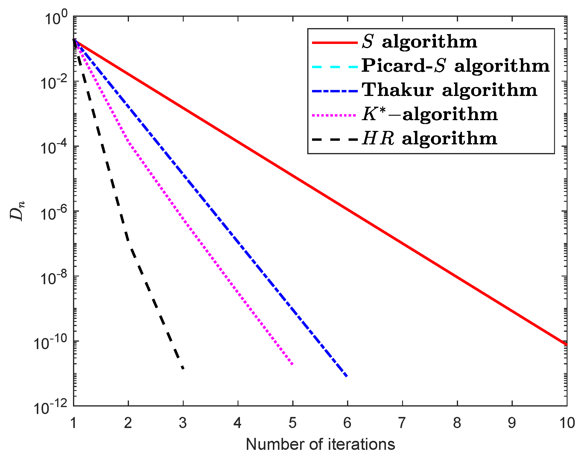
6. Numerical Experiments

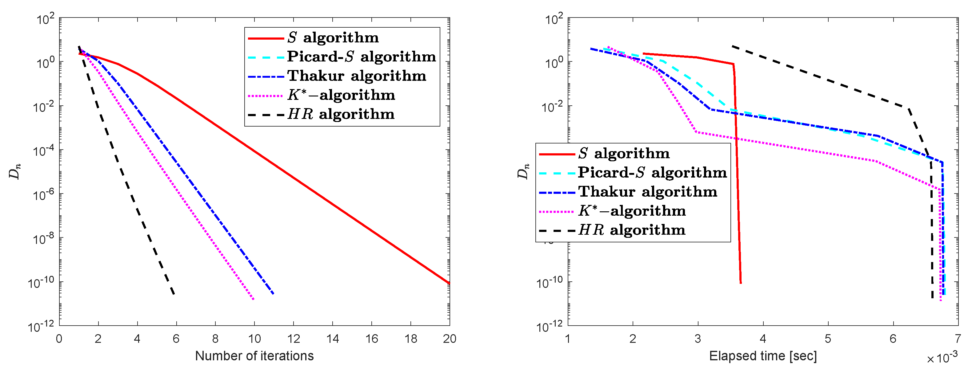
The example that follows examines how well and quickly our method performs when compared to other algorithms, while also illuminating the analytical findings from Theorem 2.
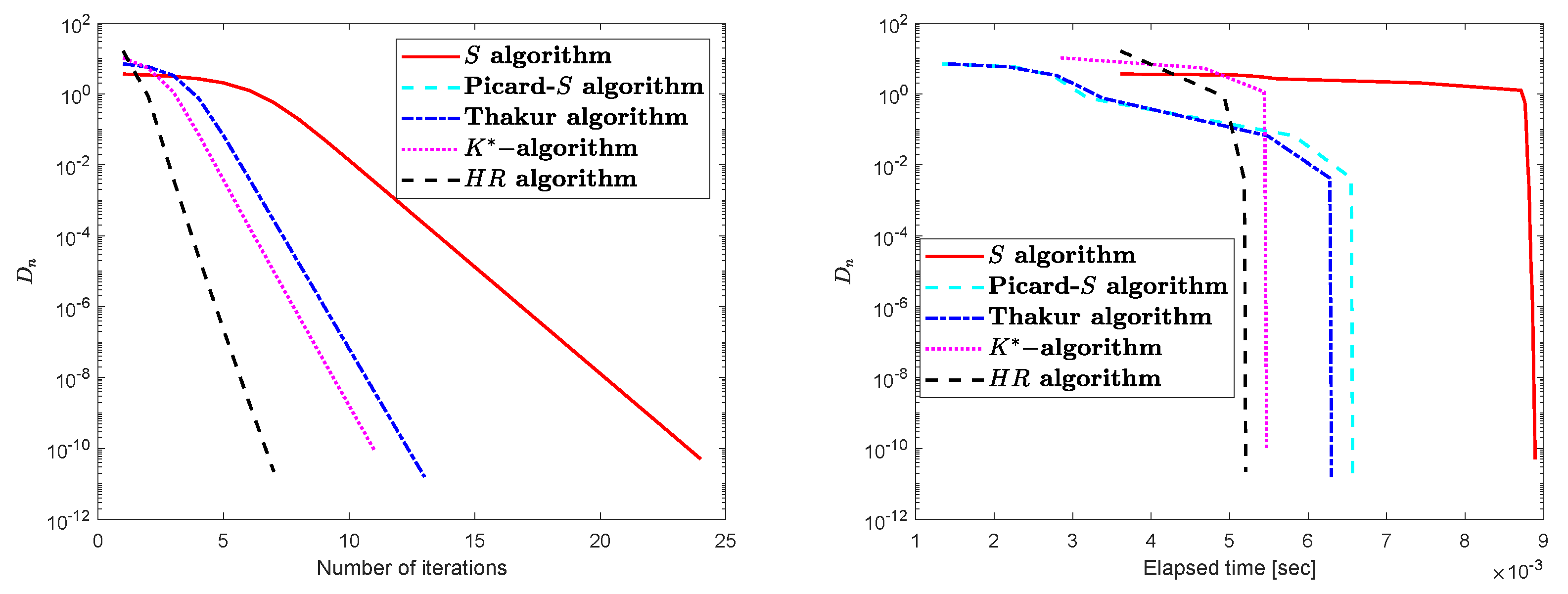
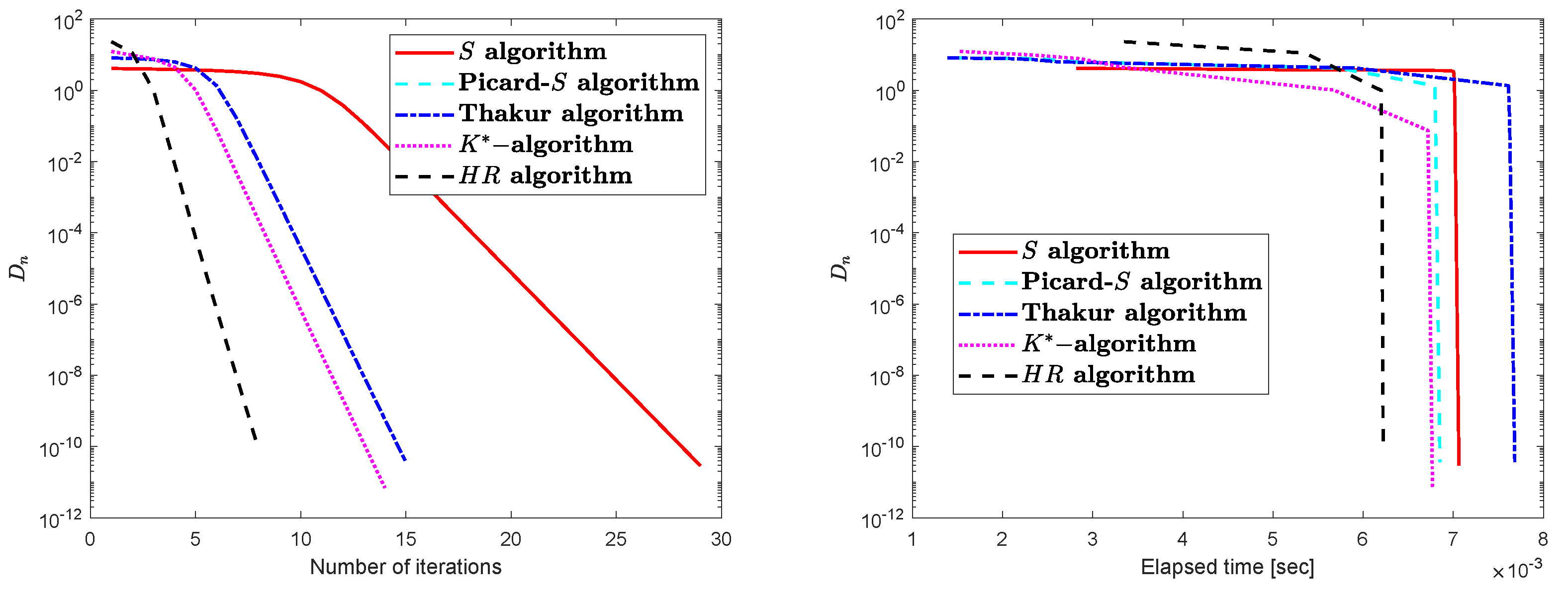
Example 2.
Let Ω = ( , ) , Θ = [ 0 , 50 ] , and : Θ Θ be a mapping described as
( ξ ) = ξ 2 9 ξ + 54 .
Obviously, 6 is a unique FP of . Consider σ j = κ j = τ j = 1 5 j + 10 , with distinct starting points. Then, we get Table 1, Table 2 and Table 3 and Figure 1, Figure 2 and Figure 3 for comparing the different iterative techniques.
The example below illustrates how our technique (7) performs better than some of the best iterative algorithms in the prior literature in terms of convergence speed under specified circumstances.
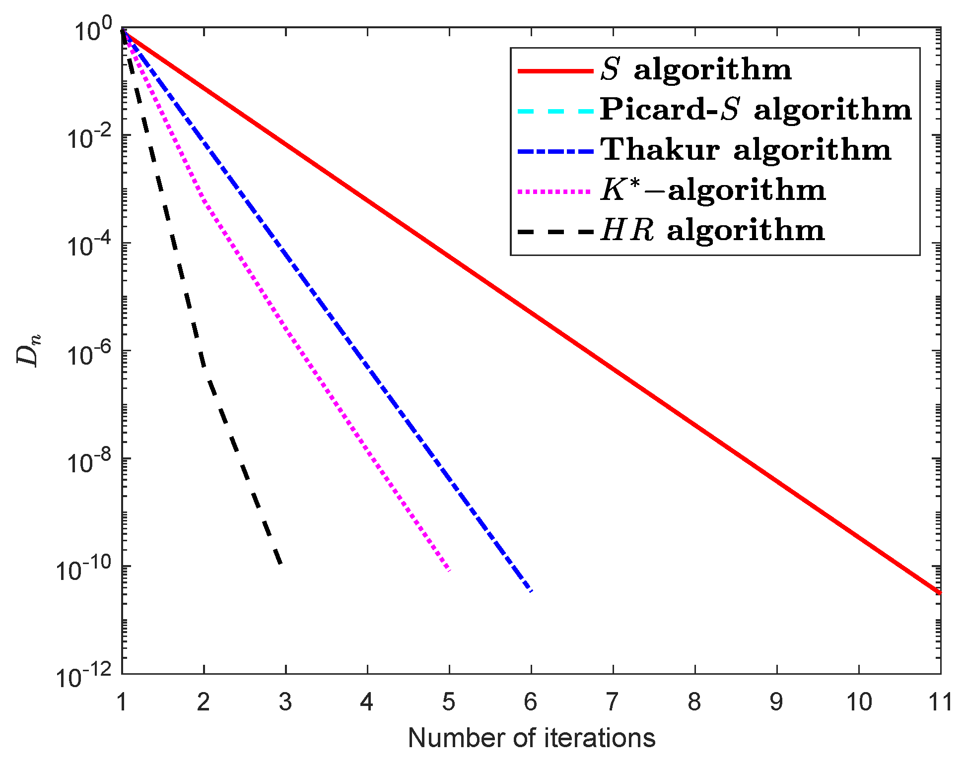
Example 3.
Define the mapping : [ 0 , 1 ] [ 0 , 1 ] by
ξ = 1 ξ , w h e n 0 ξ < 1 14 , 13 + ξ 14 , w h e n 1 14 ξ 1 .
First, we claim that the mapping ℑ is SGNM but not nonexpansive. Put ξ = 0.07 and θ = 1 14 , one has
ξ θ = ξ θ = 1 ξ 13 + ξ 14 = 0.93 183 196 = 9 2450 ,
and
ξ θ = ξ θ = 1 700 .
Hence ξ θ = 9 2450 > 1 700 = ξ θ . This proves that ℑ is not nonexpansive mapping.
After that, to prove the other part of what is required, we discuss the following cases:
(i) If 0 ξ < 1 14 , we have
1 2 ξ ξ = 1 2 ξ 1 ξ = 1 2 ξ 2 3 7 , 1 2 ,
since 1 2 ξ ξ ξ θ , then we must write 1 2 ξ 2 ξ θ . Obviously, θ < ξ is impossible. So, θ > ξ . Hence, 1 2 ξ 2 θ ξ , which implies that θ 1 2 , thus 1 2 θ < 1 . Now,
ξ θ = 13 + θ 14 1 ξ = 14 ξ + θ 1 14 < 1 14 ,
and
ξ θ = 1 14 1 2 = 3 7 .
Therefore,
1 2 ξ ξ ξ θ ξ θ < 1 14 < 3 7 = ξ θ .
(ii) If 1 14 ξ 1 , we get
1 2 ξ ξ = 1 2 13 + ξ 14 ξ = 13 13 ξ 28 0 , 169 392 .
For 1 2 ξ ξ ξ θ , we obtain 13 13 ξ 28 ξ θ , which triggers the following positions:
( p 1 ) If ξ < θ , one can write
13 13 ξ 28 θ ξ θ 13 + 15 ξ 28 θ 197 392 , 1 1 14 , 1 .
Hence,
ξ θ = 13 + ξ 14 13 + θ 14 = 1 14 ξ θ ξ θ .
So, we have
1 2 ξ ξ ξ θ ξ θ < ξ θ .
( p 2 ) If ξ > θ , one has
13 13 ξ 28 ξ θ θ 41 ξ 13 28 θ 141 392 , 1 .
Since 0 ϖ 1 and θ 41 ξ 13 28 , we have ξ 13 + 28 θ 41 ξ [ 13 41 , 1 ] .
Clearly, when 13 41 ξ 1 and 1 14 θ 1 is similar to case ( p 1 ) ; so, we shall discuss when 13 41 ν 1 and 0 ϖ 1 14 . Consider
ξ θ = 13 + ξ 14 1 θ = 14 θ + ξ 1 14 < 1 14 ,
and
ξ θ = ξ θ > 13 41 1 14 = 141 574 > 1 14 ,
which implies that
1 2 ξ ξ ξ θ ξ θ < ξ θ .
Based on the above cases, we conclude that ℑ is an SGNM.
Finally, by employing various control circumstances σ j = κ j = τ j = j j + 1 , we will describe the behavior of technique (7) and show how it is faster than the S, Tharkur, and K * iteration procedures; see Table 4 and Table 5 and Figure 4 and Figure 5.

7. Solving a Nonlinear Volterra Equation with Delay

In this section, we use the algorithm (7) that we developed to solve the following nonlinear Volterra equation with delay:
ξ ( t ) = η ( t ) + k t Π ( t , ς ) Φ t , ς , ξ ( ς ) , ξ ( ς μ ) ) d ς , t J = [ k , l ] .
with the condition
ξ ( t ) = Ξ ( t ) , t [ k μ , k ] ,
where k , l R ,   Ξ C [ k μ , k ] , R and μ , > 0 . Clearly, the space = C [ k , l ] , R , . is a BS, where the norm . is described as ξ ϑ = max t J ξ ( t ) ϑ ( t ) and C [ k , l ] , R is the space of all continuous functions defined on [ k , l ] .
Now, we present the main theorem in this part.
Theorem 7.
Suppose that Θ is a nonempty CCS of a BS ℶ and { ξ j } is a sequence generated by (7) with { σ j } , { κ j } , { τ j } [ 0 , 1 ] . Let : be an operator described as
ξ ( t ) = η ( t ) + k t Π ( t , ς ) Φ t , ς , ξ ( ς ) , ξ ( ς μ ) ) d ς , t J ,
with  ξ ( t ) = Ξ ( t ) ,   t [ k μ , k ] .  Also, assume that the statements below are true:
( s i )
the functions η : J R ,   Π : J × J R and Φ : J × J × R × R R are continuous;
( s i i )
there exists a constant A Φ > 0 such that
Φ t , ς , ξ 1 , ξ 2 ) Φ t , ς , ξ 1 * , ξ 2 * ) A Φ ξ 1 ξ 1 * + ξ 2 ξ 2 * ,
for all ξ 1 , ξ 2 , ξ 1 * , ξ 2 * R + and t , ς J ;
( s i i i )
for each t , ς J ,   2 A Φ k t Π ( t , ς ) d ς = χ < 1 .
Then the integral Equation (25) with (26) has a unique solution (US, for short) ξ ^ C [ k , l ] . Further, if ℑ is a mapping fulfilling (1), then ξ j ξ ^ .
Proof. 
First, we demonstrate that has a FP by applying the contraction principle. Recall that
ξ ( t ) ξ * ( t ) = 0 , ξ , ξ * C [ k μ , k ] , R , t [ k μ , k ] .
Next, for each t J , we can write
ξ ( t ) ξ * ( t ) = η ( t ) + k t Π ( t , ς ) Φ t , ς , ξ ( ς ) , ξ ( ς μ ) d ς η ( t ) + k t Π ( t , ς ) Φ t , ς , ξ * ( ς ) , ξ * ( ς μ ) d ς k t Π ( t , ς ) Φ t , ς , ξ ( ς ) , ξ ( ς μ ) Φ t , ς , ξ * ( ς ) , ξ * ( ς μ ) d ς A Φ k t Π ( t , ς ) ξ ( ς ) ξ * ( ς ) + ξ ( ς μ ) ξ * ( ς μ ) d ς A Φ k t Π ( t , ς ) max k μ ς l ξ ( ς ) ξ * ( ς ) + max k μ ς l ξ ( ς μ ) ξ * ( ς μ ) d ς = A Φ k t Π ( t , ς ) ξ ξ * + ξ ξ * d ς = 2 A Φ k t Π ( t , ς ) ξ ξ * d ς = χ ξ ξ * .
Since χ < 1 , we conclude that owns a unique FP and λ ( ) = { ξ ^ } because it is a contraction. Hence, the problem (25) with (26) has a US ξ ^ C [ k , l ] .
Ultimately, we prove that ξ j ξ ^ . For each ξ , ξ * Θ , one has
ξ ( t ) ξ * ( t ) ξ ( t ) ξ ( t ) + ξ ( t ) ξ * ( t ) ξ ( t ) ξ ( t ) + η ( t ) + k t Π ( t , ς ) Φ t , ς , ξ ( ς ) , ξ ( ς μ ) d ς η ( t ) + k t Π ( t , ς ) Φ t , ς , ξ * ( ς ) , ξ * ( ς μ ) d ς ξ ( t ) ξ ( t ) + A Φ k t Π ( t , ς ) ξ ( ς ) ξ * ( ς ) + ξ ( ς μ ) ξ * ( ς μ ) d ς max k μ ς l ξ ( t ) ξ ( t ) + A Φ k t Π ( t , ς ) max k μ ς l ξ ( ς ) ξ * ( ς ) + max k μ ς l ξ ( ς μ ) ξ * ( ς μ ) d ς = ξ ξ + A Φ k t Π ( t , ς ) ξ ξ * + ξ ξ * d ς ξ ξ + χ ξ ξ * .
Hence,
ξ ξ * ξ ξ + χ ξ ξ * .
It is clear that the mapping fulfilling (1) with 1 = χ < 1 and 2 = 0 . Therefore, all requirements of Theorem 1 are satisfied. Then, the sequence { ξ j } established by the iterative technique (7) converges strongly to the US of Equation (25) with (26). □

8. Conclusions and Open Problems

The effectiveness and success of iterative techniques are largely determined by two essential factors that are widely acknowledged. The two primary factors are the rate of convergence and the number of iterations; if convergence occurs more quickly with fewer repetitions, the method is successful in approximating the FPs. As a result, we have shown analytically and numerically in this work that, in terms of convergence speed, our method performs better than some of the most popular iterative algorithms, like the S algorithm [14], the Picard-S algorithm [18], the Thakur algorithm [19], and the K * algorithm [20]. Furthermore, comparison graphs of computations showed the frequency and speed of convergence and stability results. A solution to a fundamental problem served as an application that ultimately reinforced our methodology. Ultimately, we deem the following findings of this paper as potential contributions to future work:
  • The variational inequality problem can be solved using our iteration (7) if we define the mapping in a Hilbert space Ω endowed with an inner product space. This problem can be described as: find * Ω such that
    * , * 0 for all Ω ,
    where : Ω Ω is a nonlinear mapping. In several disciplines, including engineering mechanics, transportation, economics, and mathematical programming, variational inequalities are a crucial and indispensable modeling tool; see [37,38] for more details.
  • Our methodology can be extended to include gradient and extra-gradient projection techniques, which are crucial for locating saddle points and resolving a variety of optimization-related issues; see [39].
  • We can accelerate the convergence of the proposed algorithm by adding shrinking projections and CQ terms. These methods stimulate algorithms and improve their performance to obtain strong convergence; for more details, see [40,41,42,43].
  • If we consider the mapping as an α inverse strongly monotone and if the inertial term is added to our algorithm, then we have the inertial proximal point algorithm. This algorithm is used in many applications, such as monotone variational inequalities, image restoration problems, convex optimization problems, and split convex feasibility problems [44,45]. For more accuracy, these problems can be expressed as mathematical models such as machine learning and the linear inverse problem.
  • Second-order differential equations and fractional differential equations, which Green’s function can be used to transform into integral equations, can be solved using our approach. Therefore, it is simple to treat and resolve using the same method as in Section 7.

Author Contributions

H.A.H. contributed to the conceptualization and writing of the theoretical results; D.A.K. contributed to the conceptualization, writing and editing. All authors have read and agreed to the published version of this manuscript.

Funding

This research received no external funding.

Data Availability Statement

The data used to support the findings of this study are available from the corresponding author upon request.

Conflicts of Interest

The authors declare no conflict of interest.

Abbreviations

FPsFixed points
BSsBanach spaces
CCSClosed convex subset
Weak convergence
Strong convergence
ACMsAlmost contraction mappings
NIEsNonlinear integral equations
SGNMsSuzuki generalized nonexpanssive mappings
UCBSsUniformly convex Banach spaces
USUnique solution

References

  1. Berinde, V. Iterative Approximation of Fixed Points; Springer: Berlin/Heidelberg, Germany, 2007. [Google Scholar]
  2. Karapınar, E.K.; Abdeljawad, T.; Jarad, F. Applying new fixed point theorems on fractional and ordinary differential equations. Adv. Differ. Equ. 2019, 2019, 421. [Google Scholar] [CrossRef] [Green Version]
  3. Khan, S.H. A Picard-Mann hybrid iterative process. Fixed Point Theory Appl. 2013, 2013, 69. [Google Scholar] [CrossRef]
  4. Phuengrattana, W.; Suantai, S. On the rate of convergence of Mann, Ishikawa, Noor and SP-iterations for continuous functions on an arbitrary interval. J. Comput. Appl. Math. 2011, 235, 3006–3014. [Google Scholar] [CrossRef] [Green Version]
  5. Karahan, I.; Ozdemir, M. A general iterative method for approximation of fixed points and their applications. Adv. Fixed Point Theory 2013, 3, 510–526. [Google Scholar]
  6. Chugh, R.; Kumar, V.; Kumar, S. Strong convergence of a new three step iterative scheme in Banach spaces. Am. J. Comp. Math. 2012, 2, 345–357. [Google Scholar] [CrossRef] [Green Version]
  7. Berinde, V. On the approximation of fixed points of weak contractive mapping. Carpath. J. Math. 2003, 19, 7–22. [Google Scholar]
  8. Zamfirescu, T. Fixed point theorems in metric spaces. Arch. Math. 1972, 23, 292–298. [Google Scholar] [CrossRef]
  9. Imoru, C.O.; Olantiwo, M.O. On the stability of Picard and Mann iteration processes. Carpath. J. Math. 2003, 19, 155–160. [Google Scholar]
  10. Osilike, M.O.; Udomene, A. Short proofs of stability results for fixed point iteration procedures for a class of contractive-type mappings. Indian J. Pure Appl. Math. 1999, 30, 1229–1234. [Google Scholar]
  11. Mann, W.R. Mean value methods in iteration. Proc. Am. Math. Soc. 1953, 4, 506–510. [Google Scholar] [CrossRef]
  12. Ishikawa, S. Fixed points by a new iteration method. Proc. Am. Math. Soc. 1974, 44, 147–150. [Google Scholar] [CrossRef]
  13. Noor, M.A. New approximation schemes for general variational inequalities. J. Math. Anal. Appl. 2000, 251, 217–229. [Google Scholar] [CrossRef] [Green Version]
  14. Agarwal, R.P.; Regan, D.O.; Sahu, D.R. Iterative construction of fixed points of nearly asymptotically nonexpansive mappings. J. Nonlinear Convex Anal. 2007, 8, 61–79. [Google Scholar]
  15. Abbas, M.; Nazir, T. A new faster iteration process applied to constrained minimization and feasibility problems. Math. Vesn. 2014, 66, 223–234. [Google Scholar]
  16. Hammad, H.A.; ur Rehman, H.; De la Sen, M. A novel four-step iterative scheme for approximating the fixed point with a supportive application. Inf. Sci. Lett. 2021, 10, 333–339. [Google Scholar]
  17. Hammad, H.A.; ur Rehman, H.; De la Sen, M. A New four-step iterative procedure for approximating fixed points with Application to 2D Volterra integral equations. Mathematics 2022, 10, 4257. [Google Scholar] [CrossRef]
  18. Gursoy, F.; Karakaya, V. A Picard−S hybrid type iteration method for solving a differential equation with retarded argument. arXiv 2014, arXiv:1403.2546v2. [Google Scholar]
  19. Thakur, B.S.; Thakur, D.; Postolache, M. A new iterative scheme for numerical reckoning fixed points of Suzuki’s generalized nonexpansive mappings. Appl. Math. Comput. 2016, 275, 147–155. [Google Scholar] [CrossRef]
  20. Ullah, K.; Arshad, M. Numerical reckoning fixed points for Suzuki’s generalized nonexpansive mappings via new iteration process. Filomat 2018, 32, 187–196. [Google Scholar] [CrossRef] [Green Version]
  21. Karakaya, V.; Atalan, Y.; Dogan, K.; Bouzara, N.E.H. Some fixed point results for a new three steps iteration process in Banach spaces. Fixed Point Theory 2017, 18, 625–640. [Google Scholar] [CrossRef] [Green Version]
  22. Maleknejad, K.; Torabi, P. Application of fixed point method for solving Volterra-Hammerstein integral equation. UPB Sci. Bull. Ser. A 2012, 74, 45–56. [Google Scholar]
  23. Hammad, H.A.; Zayed, M. Solving systems of coupled nonlinear Atangana–Baleanu-type fractional differential equations. Bound Value Probl. 2022, 2022, 101. [Google Scholar] [CrossRef]
  24. Hammad, H.A.; Agarwal, P.; Momani, S.; Alsharari, F. Solving a fractional-Order differential equation using rational symmetric contraction mappings. Fractal Fract. 2021, 5, 159. [Google Scholar] [CrossRef]
  25. Atlan, Y.; Karakaya, V. Iterative solution of functional Volterra-Fredholm integral equation with deviating argument. J. Nonlinear Convex Anal. 2017, 18, 675–684. [Google Scholar]
  26. Lungu, N.; Rus, I.A. On a functional Volterra Fredholm integral equation via Picard operators. J. Math. Ineq. 2009, 3, 519–527. [Google Scholar] [CrossRef] [Green Version]
  27. Hammad, H.A.; De la Sen, M. A technique of tripled coincidence points for solving a system of nonlinear integral equations in POCML spaces. J. Inequal. Appl. 2020, 2020, 211. [Google Scholar] [CrossRef]
  28. Ali, F.; Ali, J. Convergence, stability, and data dependence of a new iterative algorithm with an application. Comput. Appl. Math. 2020, 39, 267. [Google Scholar] [CrossRef]
  29. Hudson, A.; Joshua, O.; Adefemi, A. On modified Picard-S-AK hybrid iterative algorithm for approximating fixed point of Banach contraction map. MathLAB J. 2019, 4, 111–125. [Google Scholar]
  30. Ahmad, J.; Ullah, K.; Hammad, H.A.; George, R. On fixed-point approximations for a class of nonlinear mappings based on the JK iterative scheme with application. AIMS Math. 2023, 8, 13663–13679. [Google Scholar] [CrossRef]
  31. Zălinescu, C. On Berinde’s method for comparing iterative processes. Fixed Point Theory Algorithms Sci. Eng. 2021, 2021, 2. [Google Scholar] [CrossRef]
  32. Berinde, V. Picard iteration converges faster than Mann iteration for a class of quasicontractive operators. Fixed Point Theory Appl. 2004, 2, 97–105. [Google Scholar]
  33. Senter, H.F.; Dotson, W. Approximating fixed points of nonexpansive mapping. Proc. Am. Math. Soc. 1974, 44, 375–380. [Google Scholar] [CrossRef]
  34. Suzuki, T. Fixed point theorems and convergence theorems for some generalized nonexpansive mappings. J. Math. Anal. Appl. Math. 2008, 340, 1088–1095. [Google Scholar] [CrossRef] [Green Version]
  35. Soltuz, S.M.; Grosan, T. Data dependence for Ishikawa iteration when dealing with contractive like operators. Fixed Point Theory Appl. 2008, 2008, 242916. [Google Scholar] [CrossRef] [Green Version]
  36. Schu, J. Weak and strong convergence to fixed points of asymptotically nonexpansive mappings. Bull. Aust. Math. Soc. 1991, 43, 153–159. [Google Scholar] [CrossRef] [Green Version]
  37. Konnov, I.V. Combined Relaxation Methods for Variational Inequalities; Springer: Berlin/Heidelberg, Germany, 2001. [Google Scholar]
  38. Facchinei, F.; Pang, J.S. Finite-Dimensional Variational Inequalities and Complementarity Problems; Springer Series in Operations Research; Springer: New York, NY, USA, 2003; Volume II. [Google Scholar]
  39. Korpelevich, G.M. The extragradient method for finding saddle points and other problems. Ekon. Mat. Metody 1976, 12, 747–756. [Google Scholar]
  40. Martinez-Yanes, C.; Xu, H.K. Strong convergence of the CQ method for fixed point iteration processes. Nonlinear Anal. 2006, 64, 2400–2411. [Google Scholar] [CrossRef]
  41. Hammad, H.A.; ur Rehman, H.; De la Sen, M. Shrinking projection methods for accelerating relaxed inertial Tseng-type algorithm with applications. Math. Probl. Eng. 2020, 2020, 7487383. [Google Scholar] [CrossRef]
  42. Tuyen, T.M.; Hammad, H.A. Effect of shrinking projection and CQ-methods on two inertial forward-backward algorithms for solving variational inclusion problems. Rend. Circ. Mat. Palermo II Ser. 2021, 70, 1669–1683. [Google Scholar] [CrossRef]
  43. Hammad, H.A.; Cholamjiak, W.; Yambangwai, W.; Dutta, H. A modified shrinking projection methods for numerical reckoning fixed points of G−nonexpansive mappings in Hilbert spaces with graph. Miskolc Math. Notes 2019, 20, 941–956. [Google Scholar] [CrossRef]
  44. Bauschke, H.H.; Combettes, P.l. Convex Analysis and Monotone Operator Theory in Hilbert Spaces; Springer: Berlin/Heidelberg, Germany, 2011. [Google Scholar]
  45. Bauschke, H.H.; Borwein, J.M. On projection algorithms for solving convex feasibility problems. SIAM Rev. 1996, 38, 367–426. [Google Scholar] [CrossRef] [Green Version]
Figure 1. The suggested algorithm ( H R algorithm) at ξ = 1 .
Axioms 12 00715 g001
Figure 2. H R algorithm at ξ = 23 .
Axioms 12 00715 g002
Figure 3. H R algorithm at ξ = 41 .
Axioms 12 00715 g003
Figure 4. Comparison of the suggested algorithm visually ( H R algorithm) at ξ = 0.30 .
Axioms 12 00715 g004
Figure 5. Comparison of the suggested algorithm visually ( H R algorithm) when ξ = 0.80 .
Axioms 12 00715 g005
Table 1. Example 2: ( H R algorithm) at ν = 1 .
Iter (n)S AlgorithmPicard-S AlgorithmThakur Algorithm K * Algorithm HR Algorithm
18.700917049817467.169219208494547.169147723744436.360594433091946.00727524833131
27.165262321120996.109771779575586.109759231180576.014684666444526.00002780412529
36.390882324693956.007144036073756.007143169809886.000654500580636.00000018328059
46.109315649225126.000447210720236.000447156307486.000031685260566.00000000153606
56.028234169568836.000027932253766.000027928854546.000001613160226.00000000001474
66.007116363712716.000001744716056.000001744503736.000000084911516.00000000000015
76.001782209208796.000000108993716.000000108980456.00000000457683
86.000445635258876.000000006809596.000000006808766.00000000025113
96.000111390899006.000000000425476.000000000425426.00000000001397
106.000027841789336.000000000026596.000000000026586.00000000000079
116.000006959057786.000000000001666.00000000000166
126.00000173945939
136.00000043479852
146.00000010868515
156.00000002716811
166.00000000679132
176.00000000169767
186.00000000042438
196.00000000010609
206.00000000002652
Table 2. Example 2: H R algorithm at ξ = 23 .
Iter (n)S AlgorithmPicard-S AlgorithmThakur Algorithm K * Algorithm HR Algorithm
119.356315255502915.951805633560315.951779858674512.58772672843916.85064626172682
215.937728080845910.154742977984810.15470637463717.213109217957456.00404110670722
312.82162673898216.836374150133816.836352320232176.077734366898896.00002666859578
410.14536650061616.070610761318326.070607995982136.003859981514406.00000022350839
58.099048940913846.004531821229156.004531636991286.000196775628436.00000000214472
66.833428643384756.000283566493496.000283554939826.000010358331496.00000000002245
76.260449089315796.000017716559836.000017715837896.000000558328306.00000000000025
86.070325430855646.000001106882546.000001106837446.00000003063582
96.017961133385126.000000069159446.000000069156626.00000000170455
106.004514344164136.000000004321396.000000004321226.00000000009591
116.001129942204176.000000000270036.000000000270026.00000000000545
126.000282535119296.000000000016876.00000000001687
136.000070629203296.000000000001056.00000000000105
146.00001765533615
156.00000441334114
166.00000110322227
176.00000027578013
186.00000006893931
196.00000001723354
206.00000000430809
216.00000000107696
226.00000000026923
236.00000000006730
246.00000000001683
Table 3. Example 2: H R algorithm at ξ = 41 .
Iter (n)S AlgorithmPicard-S AlgorithmThakur Algorithm K * Algorithm HR Algorithm
136.919539390231032.935945929557532.935941037249428.677705043015918.0010100671820
232.918520904862325.185471315982025.185463782191819.11840502755376.99692674147933
328.996665225549817.943365890819317.943356389804811.53961256860706.00870649597241
425.170164917241111.686380449982011.68636974084167.090982450368866.00007316294814
521.46708774707577.497070089135867.497061912315176.078772852880806.00000070206652
617.93137574957346.156129407755426.156127750110776.004260755828646.00000000734890
714.63203756977766.010356599876806.010356479457276.000230004995556.00000000008173
811.67812757748426.000649667151106.000649659554116.000012621548996.00000000000095
99.233715524924756.000040602315346.000040601840406.00000070225384
107.493505756008706.000002537055776.000002537026096.00000003951159
116.535249547963296.000000158533116.000000158531256.00000000224357
126.155637699644876.000000009906566.000000009906456.00000000012838
136.040782947349026.000000000619076.000000000619066.00000000000739
146.010324068405196.000000000038696.000000000038696.00000000000043
156.002589036499636.000000000002426.00000000000242
166.00064771546926
176.00016194664418
186.00004048534517
196.00001012070523
206.00000253001219
216.00000063246434
226.00000015810715
236.00000003952473
246.00000000988071
256.00000000247007
266.00000000061749
276.00000000015437
286.00000000003859
296.00000000000965
Table 4. Example 3: Comparison of the suggested algorithm numerically ( H R algorithm) at ξ = 0.30 .
Iter (n)S AlgorithmPicard-S AlgorithmThakur Algorithm K * Algorithm HR Algorithm
10.9189256198347110.9926296018031560.9926296018031560.9993852878901710.999999491973463
20.9926593811898100.9999393337288410.9999393337288410.9999974388744830.999999999938058
30.9993341876740340.9999994997653450.9999994997653450.9999999862056530.999999999999984
40.9999395596480300.9999999958718430.9999999958718430.999999999916912
50.9999945109726270.9999999999659180.9999999999659180.999999999999467
60.9999995013678290.9999999999997190.999999999999719
70.999999954695558
80.999999995883263
90.999999999625887
100.999999999966000
110.999999999996910
Table 5. Example 3: Comparison of the suggested algorithm numerically ( H R algorithm) when ξ = 0.30 .
Iter (n)S AlgorithmPicard-S AlgorithmThakur Algorithm K * Algorithm HR Algorithm
10.9819834710743800.9983621337340350.9983621337340350.9998633973089270.999999887105214
20.9983687513755130.9999865186064090.9999865186064090.9999994308609960.999999999986235
30.9998520417053410.9999998888367430.9999998888367430.9999999969345890.999999999999996
40.9999865688106730.9999999990826320.9999999990826320.999999999981536
50.9999987802161390.9999999999924260.9999999999924260.999999999999881
60.9999998891928510.9999999999999380.999999999999938
70.999999989932346
80.999999999085170
90.999999999916864
100.999999999992444
Disclaimer/Publisher’s Note: The statements, opinions and data contained in all publications are solely those of the individual author(s) and contributor(s) and not of MDPI and/or the editor(s). MDPI and/or the editor(s) disclaim responsibility for any injury to people or property resulting from any ideas, methods, instructions or products referred to in the content.

