Review

Review of Nonlocal-in-Time Damping Models in the Dynamics of Structures

1
Research and Education Center after Zolotov, Moscow State University of Civil Engineering, 129337 Moscow, Russia
2
Department of Systems’ Automation Design, Russian University of Transport (RUT) (MIIT), 127994 Moscow, Russia
3
Institute of Applied Mechanics, Russian Academy of Sciences, 125040 Moscow, Russia
*
Author to whom correspondence should be addressed.
Axioms 2023, 12(7), 676; https://doi.org/10.3390/axioms12070676
Submission received: 3 June 2023 / Revised: 4 July 2023 / Accepted: 7 July 2023 / Published: 10 July 2023
(This article belongs to the Special Issue Applied Numerical Analysis in Civil Engineering)

Abstract

:
In the present paper, the nonlocal-in-time damping models, called “damping-with-memory” models, are reviewed. Since such models do not involve the distribution along the longitudinal coordinate, they are easily adjustable for the FEM (Finite Element Model) algorithm, which is a big advantage due to the fact that FEM is the most-used method in engineering calculations. Within damping-with-memory models, the internal damping of a structure at the current time, is assumed to be dependent not only on the instant strain-rate magnitude or displacement-velocity magnitude but also on the strain-rate or velocity values along the previous time history. The greater the gap between the two time points, the lower the influence that one of them has on the other. To implement a composite beam vibration simulation involving damping with memory, the equation of motion of a structure written in the matrix form could be solved using the central difference method. The models constructed could be calibrated based on 3D numerical simulation data with the least squares method. It has been shown that the results obtained using the implementation of a calibrated damping-with-memory model within the 1D finite-element beam algorithm are in good correlation with those given by the 3D-FEM numerical simulation data.
MSC:
74D05; 74H15; 74H45; 74K10

1. Introduction

The problem of modeling the vibrations in structural elements made of modern composites and nanomaterials is a significant challenge. Unlike traditional building materials, such as metals, composites are highly heterogeneous and anisotropic [1,2].
One of the features of such structural materials is that the physical properties of matrices and binders that comprise their basis differ significantly. By using various combinations of parameters and orientations of inorganic and organic materials in manufacturing composites, it is possible to control their properties and to achieve the desired characteristics and parameters, allowing one to solve different problems in a wide variety of manufacturing industries [1,2].
Classic hypotheses are often not enough to describe the behavior of such materials. Hence, it is suggested that mathematical models are especially flexible and controllable to simulate the dynamic response of structures considering their orthotropic or other types of anisotropy properties [3,4].
The aim of this review is to overview recent publications and results addressing the application of the models with nonlocal-in-time damping for solving dynamics problems of structural mechanics.

2. Mathematical Modeling of the Internal Friction

The problem of modeling the internal friction in composite or even homogeneous materials is especially challenging. Currently, this problem does not have an unambiguous solution. Internal friction in a material means energy-irreversible processes that accompany the cyclic deformation of bodies [5,6,7]. It is believed that the irreversibility of these processes is characterized by the fact that part of the deformation energy for each cycle is converted into heat or electricity and dissipated. In the literature, there exist several measures of internal friction [5], among them: the tangent of the mechanical loss angle; specific energy dissipation; and the inverse value of the quality factor, etc.
There have been over one hundred and fifty years of research into the issues of internal friction in a deformable material [8,9,10,11,12,13]. During this period, many different and often contradictory theories and models have been developed that describe the process of the dissipation of the energy of vibrations. For example, according to the Kelvin–Voigt hypothesis [14], energy losses due to internal friction in a material are proportional to the rate of change in cyclic deformations. On the contrary, in the theory developed by Maxwell, the internal absorption parameter is inversely proportional to the vibration frequency [15], while Sorokin’s hypothesis of complex stiffness [7] is frequency independent.
None of the currently existing hypotheses is universal or applicable to various materials within a wide frequency range. It is clear that only a stable correspondence to actual dynamic processes could confirm the reliability of one theory or another.
The monograph in Reference [16] was devoted to the problems of vibration and noise in various fields of mechanical and civil engineering, wherein different ways of describing various types of damping were considered. Particular attention was paid to models of viscoelastic damping, which determine the behavior of composites: polymer and vitrified materials. At the same time, it was noted in Reference [16] that during the manufacturing of composites, as a rule, producers do not ascribe to the goal of achieving high damping characteristics. Therefore, in laboratory or ambient experiments, it is difficult to separate the pure damping effects from the effects arising from the nonlinear behavior of the material. Thus, it is necessary to describe the influence of viscoelastic damping on the dynamic behavior of structures.
Adhikari [17] presented an analysis of complex systems with damping. The main object of research was a multiple-degree-of-freedom system with viscous and/or non-viscous internal friction. The theory of a viscoelastic-hereditary medium was used as the theory of inviscid friction, and its particular case was the model of viscous friction in Reference [18].

3. Non-Classical Models of Composite and Viscoelastic Materials

Before we focus on internal friction modeling, the non-classical models of composite materials considering general deformation should be discussed. Various conceptual and mathematical models have been proposed to take into account the peculiarities of composite and viscoelastic materials’ response under loading, among them: gradient models [19]; mathematical models involving the apparatus of fractional calculus [20,21,22]; nonlocal models [23]; and nonlocal models via operators of fractional order [24,25,26,27].
Flügge, in his book on viscoelasticity [28] (see p. 74), noted that “The response q(x1) at some point x1 obviously depends, of course, not only upon the local value w(x1) of the deflection but also upon that at neighbor points x2. Their influence decreases as the distance |x1x2| increases.” Thus, Flügge came to the conclusion that in order to solve practical engineering problems, it is necessary to study a class of models that are now called nonlocal.
Lei et al. [4] emphasized that from a physical point of view, the need to take into account nonlocal elastic or damping properties arises when it is expedient to model a two-dimensional or spatial element as a one-dimensional one. Therefore, such an approach has many potential applications in engineering structures with nonlocal energy dissipation mechanisms.
In 1972, Eringen and Edelen [29] proposed a nonlocal model of the elastic properties of a structural material, which was further developed by many researchers, among them References [30,31,32].
In 1975, Ahmadi studied a linear theory of nonlocal viscoelastic material in Reference [33] and obtained the constitutive equations for nonlocal Kelvin–Voigt, Maxwell, and Boltzmann–Volterra viscoelastic materials. It was shown that the simple viscoelastic materials, in fact, are nonlocal-in-time properties.
Baretta et al. [34] suggested a combination of Eringen’s nonlocal elasticity model and the fractional derivative model of viscoelasticity to solve the problem of bending of Euler–Bernoulli beams in porous viscoelastic materials.
Another way to generalize the linear relationship between stress and strain was proposed by Boltzmann [35] and Volterra [36], who developed the theory of a viscoelastic medium with heredity, according to which the strain at any given time depends on all that has happened before, i.e., on the whole stress history. The final deformation at the considered moment of time is represented by the sum of the deformations caused by each of the previously acting forces, considering the decrease in their influence over the current time. The degree of such a decrease is described by a memory function that monotonically decreases with an increase in the argument, which characterizes the hereditary properties of the material. The type of hereditary kernel should be selected based on experimental data.
A great contribution to the development of the hereditary theory of elasticity was made by Academician Rabotnov [13,37,38]. The fractional–exponential kernel of the hereditary elasticity proposed by him [37] enabled results that are in good agreement with the results of testing polymeric materials to be obtained.
The monograph in Reference [39] was devoted to the construction of nonlocal models (Kunin chains). It has been noted that nonlocality could be of a physical or geometric nature. In the first case, the scale parameter corresponds to the characteristic size of the material’s microstructure. In the second case, it is due to the approximate consideration of such parameters as the thickness of a structural element (rod or plate), while the nonlocal model serves for an effective approximate description of the behavior of a homogeneous three-dimensional medium. The book [39] presented in detail the construction of the mathematical apparatus of nonlocal theories and also noted a number of inherent ambiguities, such as the ambiguity of the certainty of energy density, stresses, etc.
Nonlocal elasticity models were used for theoretical studies of nanorod and nanoplate systems in References [40,41]. The nonlocal elasticity model was applied to the wave propagation modeling in Reference [42].
Bažant and Jirásek [23] reviewed the progress in nonlocal models of the integral type and discussed their physical justifications, advantages, and numerical applications. It has been noted that “the term nonlocal has in the past been used with two senses, one narrow and one broad. In the narrow sense, it refers strictly to the models with an averaging integral. In the broad sense, it refers to all the constitutive models that involve a characteristic length (material length), which also includes the gradient models. This broad sense stems from the realization that some gradient models are derived as approximations to the nonlocal averaging integrals and that for all the gradient models, the gradient, in fact, includes a dependence on the immediate (infinitely close) neighborhood of the point under consideration”. An interested reader could find a state-of-the-art in the field of application of such nonlocal models in mechanics in Reference [23].
Potapov [43,44] considered the problem of the dynamic stability (in the sense of Lyapunov) of a composite rod with the simultaneous application of the hypotheses of nonlocal elasticity and nonlocal damping. Although this approach, on the one hand, makes the model very flexible, which is very important when working with orthotropic and anisotropic materials, on the other hand, the simultaneous consideration of both nonlocal elasticity and nonlocal damping makes the model quite complex from a mathematical point of view.
Suppose that in order to achieve the required calculation accuracy, it is sufficient to use either only the hypothesis of nonlocal elasticity or only the hypothesis of nonlocal damping. Further, we would focus on the hypothesis of nonlocal damping.

4. Nonlocal Damping Models

For the first time, a damping model, nonlocal-in-spatial coordinates, was proposed by Russell [45] for the dynamic analysis of a composite beam.
Banks and Inman [3] examined four damping models using the example of vibrations of a composite cantilever beam with a concentrated mass at the free end. The beam was made of fiberglass-reinforced plastic. In so doing, the reinforcement was arranged in the longitudinal and transverse directions. It was noted that this material possesses damping properties that are different from those of homogeneous materials. It was assumed that the behavior of the beam corresponded to the Bernoulli hypothesis, and the torsional, shear, and longitudinal displacements were negligible.
Three models presented in Reference [3] describe internal friction: the Voigt model; time hysteresis; and spatial hysteresis. The model called temporary hysteresis in Reference [3] is similar to the theory of the medium with heredity, where the system’s response to external influences that took place in the past affects its dynamic behavior in the present.
Spatial hysteresis is similar to the damping model nonlocal-in-coordinates [45]. This model is based on the assumption that the energy losses during lateral vibrations of the beam are associated with the fact that the internal friction in the material is caused by the rotation of the sections relative to each other. Moreover, not only the considered cross-section of the beam affects the process of internal damping but also the cross-sections adjacent to it. In this case, a kernel function or an influence function should be introduced, which is the law of a decrease in the influence of cross-sections on each other with an increase in the distance between them.
The fourth model in Reference [3] described external viscous damping. In other words, it assumed that the vibration damping process was associated with the friction of the structure against the external medium. The damping forces were considered proportional to the displacement rates. This hypothesis is convenient for practical applications.
Some combinations of these models are also considered in Reference [3]. It is noted that the described approaches are based on physical considerations. Damping models are involved in the equation of bending vibrations of the Euler–Bernoulli beams. In this case, the boundary conditions were chosen so that they could be used with different damping models.
The selection of the parameters for damping models was carried out in Reference [3] according to the experimental data using the least squares method. The parameters obtained in this way were utilized in integrodifferential equations to simulate the dynamic response of the system. The vibration process modeled in such a way was compared with experimental data. It has been shown that the spatial hysteresis used as a model of internal friction in combination with external viscous damping gives the best agreement with the experiment.
Banks and Inman [3] emphasized that the intuitive idea physically confirmed that external damping is significantly manifested at lower vibration frequencies, while internal friction has a stronger effect on the vibration process at higher frequencies. It is also noted that the proposed damping models cannot be constructed using standard damping coefficients obtained by modal analysis since they completely hide the physics and the mechanism of the damping process. The natural frequencies obtained as a result of mathematical modeling for the considered beam were compared with those measured experimentally. It has been noted that the results of numerical calculations of a beam with plastic fiberglass reinforced, according to the Euler–Bernoulli theory, coincide well with the experimental data, and there is no need to use the Timoshenko beam model.
For the dynamic analysis of Euler–Bernoulli beams and Kirchhoff plates, Lei et al. [4] suggested using a nonlocal damping model, which includes spatial and temporal hysteresis. In contrast to the usual local models, the damping forces are calculated as the average of the velocity field in a certain region determined by the kernel function. The resulting integro-differential equation of motion in partial derivatives is solved by the Bubnov–Galerkin method.
It was emphasized by the authors of [4] that a new nonlocal damping model proposed for analyzing the dynamic characteristics of bending beams under various boundary conditions is the generalization of the classical model of viscous friction and could be applied in the calculations of engineering structures when it is important to take into account the nonlocal mechanism of energy dissipation during vibrations. Such structures include those with a viscoelastic damping coating, structures on viscoelastic foundations, structures made of composite and nanomaterials, etc.
Within such an approach, it is assumed that damping at some point of the bar with coordinate x 1 , measured along its axis, is considered dependent not only on the local value of the rate of deformation change ε ˙ ( x 1 , t ) at the same point x 1 but also on the value of the rate of change in deformations at neighboring points at some area adjacent to this point. The less the degree of influence of the damping properties of the points under consideration on each other is, the greater the distance between them.
The approach proposed in Reference [4] was further utilized for solving different engineering problems, among them: a modal analysis [46] and a finite element analysis of the Euler–Bernoulli beams with internal nonlocal damping [47,48]; a finite element method for elastic beams resting on nonlocal foundations [49]; and Timoshenko beams with internal nonlocal damping [50].
Reference [48] concluded that “the external damping parameters have simple effects on the natural frequencies and the dependence with nonlocal parameter is not strong”. Hence, the nonlocal-internal and -external damping parts in the equation of motion can be modeled independently. Therefore, the modal analysis technique for the nano-scale Euler–Bernoulli beams was proposed with the consideration of damping that is nonlocal both in time and space in Reference [51].
A novel dynamic finite-element approach for bending vibrations of damped nonlocal-in-space beams on an elastic foundation was proposed in Reference [51]. Both internal and external damping mechanisms were employed. The stiffness and mass matrices of the nonlocal beam were obtained using the conventional finite element method. The scale factor of the nonlocal model was not determined by any experimental data, and for numerical examples, it was considered from 0 to 2 nm [51].
Emphasizing the physical significance of nonlocal models, Gonzales et al. [52] utilized the approach by Lei et al. [4,46,47,48,49,50] for treating the Euler–Bernoulli beams with separate areas of nonlocal properties via the Galerkin method. In Reference [53], the models of spatial and spatiotemporal nonlocal-internal damping were applied to the nonlinear seismic analysis of a four-story frame. It was shown that nonlocal damping models do not exhibit spurious damping properties as exhibited by the global damping models on the onset of inelasticity.
We should also mention the series of theoretical papers [54,55,56,57,58,59,60] which are devoted to the nonlocal energy damping model with linear and nonlinear terms, wherein the energy dissipation is considered in Euler–Bernoulli beams and Kirchhoff plates with different boundary conditions. The authors of [54,55,56,57,58,59,60] declared that the model is suitable for flight structures, pipes, and plate dynamic simulation, including supersonic flatter.
The significant contribution to the development and application of the nonlocal damping theory to practical engineering problems was made by Potapov [61,62]. In 2012, he implemented the nonlocal-in-space damping model to the problem of the stability of vertical columns subjected to longitudinal force [61]. The solution was found using the Bubnov–Galerkin and the Runge–Kutta fourth-order methods. Further, this approach was utilized for modeling nonlinear systems, and the problem of shallow arch stability was solved [62].
To this purpose, instead of the traditional Voigt hypothesis
σ = E ε + E t κ   ε ˙ ,
where σ and ε are the normal stress and longitudinal strain, respectively, ε ˙ is the strain rate, E is Young’s modulus, and t κ is the retardation time, the following relationship was used:
σ x , t = E ε x , t + χ 0 l C x θ ε ˙ θ , t d θ ,
where C ( x θ ) is a function that describes the decrease in the influence of points with coordinates x and θ on each other, and χ is the dynamic viscosity.
The research started by Potapov and his collaborators [61,62,63,64] on modeling internal damping nonlocal-in-spatial coordinates was further developed in References [65,66], resulting in a technique allowing one to calibrate the model parameters using the data of numerical simulations of the vibrations of a composite beam in a three-dimensional configuration, taking its orthotropic properties into account. The results presented in References [65,66] indicate that a one-dimensional nonlocal model could be used instead of a detailed classical spatial computational model.
Although the nonlocal-in-space damping model shows good agreement with the results of numerical experiments [65,66], its embedding into the algorithm of a numerical calculation method, for example, the finite element method, is rather difficult and, to some extent, farfetched. This is due to the fact that the kernel function describing the character of the decrease in the influence of neighboring points of an element on each other can step over the boundaries of finite elements.
But since the finite element method is the predominant method of analysis in engineering practice, it becomes necessary to construct a model that is flexible enough to describe the dynamic behavior of a composite material and, at the same time, is easily integrated into the finite element method algorithm. Such a model similar to that for damping nonlocal-in-time, proposed in Reference [3], was developed further by Sidorov et al. [67], with the only difference that the authors of Reference [67] assumed that damping at the current moment of time t depends not only on the instantaneous value of the rate of change in deformations at this moment of time ε ˙ ( t ) but also on the value of the rate of change in deformations at the previous moments of time τ . Moreover, the less the effect of the value of the rate of change in deformation at a certain moment of time τ is, the longer the time interval between τ and the current moment t   i s . That is why we will refer to this model as damping-with-memory.
See Table 1 for the main classical and nonlocal models of internal friction for solids and structures. The main types of kernel functions C x θ and G t τ utilized in the spatial and temporal nonlocal models, respectively, are presented in Table 2, where μ and l0 are the characteristic parameters of the damping material [50], and γ is the coefficient of inelastic reaction due to Sorokin [3].

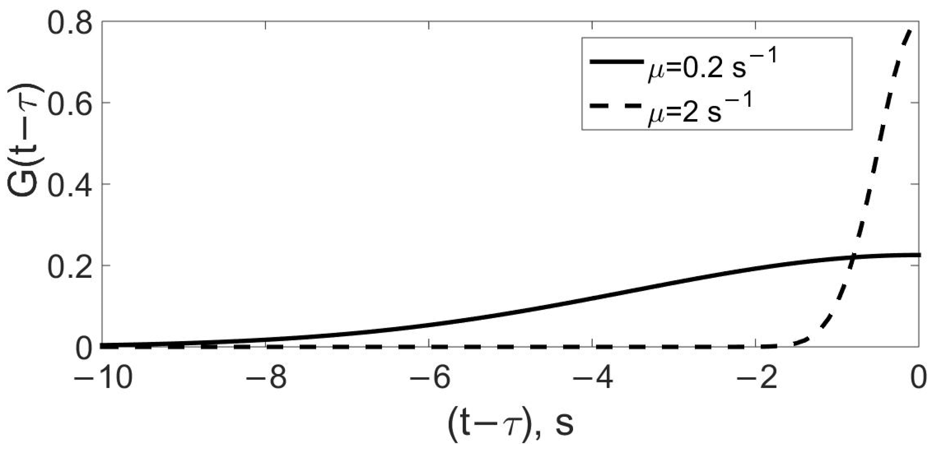
5. Damping-with-Memory Model

Within the algorithm of the finite element analysis, the equilibrium equation of a structure deformed during its motion could be represented in the matrix form as follows [71]:
M V ¨ t + D V ˙ t + K V t = F t ,
where V ( t ) is the displacement vector, M is the mass matrix, K is the stiffness matrix of the finite element model, F ( t ) is the load vector, while D is the damping matrix.
The stiffness and mass matrices of the i-th beam element have the form [71]:
K i = 12 E I l 3 6 E I l 2 12 E I l 3 6 E I l 2 6 E I l 2 4 E I l 6 E I l 2 2 E I l 12 E I l 3 6 E I l 2 12 E I l 3 6 E I l 2 6 E I l 2 2 E I l 6 E I l 2 4 E I l ,
M i = ρ A l 420 156 22 l 54 13 l 22 l 4 l 2 13 l 3 l 2 54 13 l 156 22 l 13 l 3 l 2 22 l 4 l 2 ,
where l is the element length, I is the moment of inertia, and ρ is the material density.
Assuming that the memory model of material damping depends on the values of the strain rate, its damping matrix could be deduced according to the requirement of stationary state of the full energy of the vibrating system. Thus, the dissipation of energy during deformation of a finite element under dynamic loading will be represented by a dissipative function Φ D [72,73]:
Φ D = 1 2 χ ε ˙ 2 ,
where the coefficient defining material viscosity χ could be obtained as follows:
χ = E t κ ,
and t κ is the retardation time (sometimes it is called the delay time [72]) which could be determined in terms of the damping coefficient (critical fraction) ξ c r and the first natural frequency of the system ω [72,73]
t   κ = 2 ξ c r ω .
Energy dissipation through the material of the whole system could be presented as the summation of energy dissipation Φ D i through each finite element:
Φ D = i 1 N Φ D i ,
where i is the finite element number ( i = 1 ,   2 ,   ,   N ) , N is the number of elements in the whole FE computational model, which, in the case of a bent beam, has the form [68]
Φ D i = 1 2 l A χ ε ˙ b 2 d A d z ,
where A is the element’s cross-section area, z is the longitudinal coordinate, l is the element length, and ε ˙ b is the bending-induced axial strain rate.
Bending-induced axial strain for the Euler–Bernoulli beam is as follows [73]:
ε b = 1 R y = d 2 v d z 2 y ,
where R is the radius of curvature of the beam’s neutral layer, y is the distance to the considered beam fiber from its neutral layer, and v is the transverse displacement.
Then Equation (10) is reduced to
Φ D i = 1 2 I χ l d 2 v ˙ d z 2 2 d z .
Within the FEA, the transverse displacements could be approximated along the beam element with cubic shape function:
N v T = 1 3 ξ 2 + 2 ξ 3 l ( ξ 2 ξ 2 + ξ 3 ) 3 ξ 2 2 ξ 3 l ( ξ 2 + ξ 3 ) ,
where ξ = z l is the reduced local longitudinal coordinate.
Considering (13), the Expression (12) could be reduced to
Φ D i = 1 2 I χ 0 1 A v N v T A v N v v ˙ i 2 l d ξ .
where v ˙ i = v ˙ 0 φ ˙ 0 v ˙ l φ ˙ l are nodal velocity vectors during bending. In so doing, v ˙ 0 and v ˙ l are the velocities of the transverse displacements at the initial and terminal points of each i-th element, and φ ˙ 0 and φ ˙ l are velocities of rotation displacements, and A v = d 2 l 2 · d ξ 2 .
The requirement for the stationary state of the full energy of the vibrating system
Φ D v ˙ = 0
gives us the D V ¯ ˙ term in the equilibrium equation in Motion (3).
The beam’s damping matrix D is obtained by topological summation of the element’s damping matrices D i as follows:
D i = I χ 0 1 A v N v T A v N v l d ξ ,
or
D i = χ · 12 I l 3 6 I l 2 12 I l 3 6 I l 2 6 I l 2 4 I l 6 I l 2 2 I l 12 I l 3 6 I l 2 12 I l 3 6 I l 2 6 I l 2 2 I l 6 I l 2 4 I l .
To construct the damping-with-memory model, Equation (3) should be represented as follows: [67]
M V ¨ t + D 0 t G t τ V ˙ τ d τ + K V t = F t ,
where G ( t τ ) is the kernel function which describes the decrease in the influence of the motion velocity at the moment τ on damping at the current moment t. The kernel function should be normalized to satisfy the following condition:
t G t τ d τ = 1 .
Considering (19), the error function could be used as the kernel function
G t τ = 2 μ π e μ 2 t τ 2 ,
where μ is a parameter of the model that determines the rate of decay of the influence of the nonlocal damping over distance, i.e., the parameter characterizing the level of damping temporal nonlocality [68]. The higher is μ , the closer the model is to the classic local one (Figure 1).

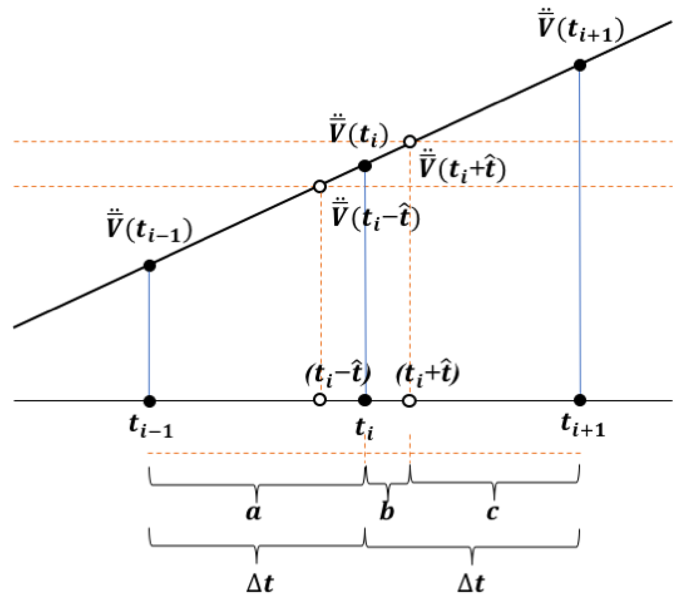
6. Equilibrium Equation Solving with the Method of Central Differences

To solve the dynamic equilibrium equation, the method of the central differences could be adopted [69], what allows one to reduce Equation (18) to the following form [67]:
1 Δ t 2 M V i + 1 2 V i + V i 1 + D 2 Z + 1 2 Δ t D V i + 1 V i + K V i t = F i ,
where i = 1 ,   2 ,   3 is a number of the considered moments in time t , and Δ t   is the time step.
In Equation (21), the vector has the form
Z = j = 1 i 2 μ π e μ 2 t τ Δ t / 2 2 V j V j 1 ,
where τ = j   Δ t , and t = i Δ t .
From Equation (21), it follows that the displacement vector V i + 1 could be calculated in terms of V i and V i 1 as follows:
V i + 1 = Q F i Q 1 V i Q 2 V i 1 Q 3 Z ,
where
Q = 1 Δ t 2 M + 1 2 Δ t D 1 , Q 1 = Q 2 Δ t 2 M 1 2 Δ t D + K , Q 2 = Q 1 Δ t 2 M ,           Q 3 = 1 2 Q D .
At the first step, i.e., for i = 1 , V 0 = 0 and V 1 = 0 are taken as the initial conditions.
The solution obtained by the explicit scheme turned out to be quite unstable and demanding in a sense of calculation time. For the explicit scheme, the maximum allowed time increment was 0.001 s. For the larger time steps, the finite element model fell apart [67]. Thus, it was further decided to use the Newmark method (the implicit scheme) instead, since it has been found in Reference [69] that the implicit scheme allows the maximum time increment of 0.01 s, i.e., 10 times larger in comparison to the central difference method.

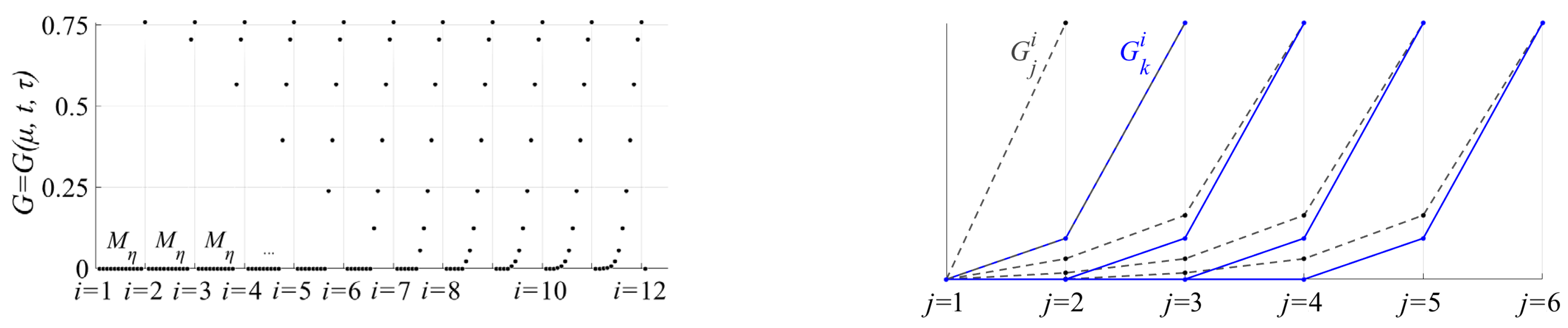
7. Modified FEA Model Considering Nonlocal Damping Solved by the Implicit Scheme

In order to make the modal more flexible and controllable, the additional terms have been added to the FEA equation of Motion (3) [69,70]:
M V ¯ ¨ t + α D V ¯ ˙ t + 1 α D t 0 t t G μ , t τ V ¯ ˙ τ d τ + K V ¯ t = F ¯ t .
Similar to Reference [4], the material had separate parts of locality and nonlocality, the damping properties were also divided into nonlocal and local parts, and α was the coefficient of nonlocality, i.e., the parameter assigning the share of local properties of the model ( 0 < α < 1 ).
The equation of motion (25) could be solved using the modified Newmark method [71]. The computational scheme for the vertical displacements of the beam is as follows:
V ¯ t i + 1 = K e f 1 R e f t i + 1 ,
where the effective stiffness matrix K e f and the effective load vector R e f t i + 1 have the following forms:
K e f = 1 a · t M + α t D + K ,
R e f t i + 1 = F t i + 1 + Q 1 V ¯ t i + t V ¯ ˙ t i + t b V ¯ ¨ t i +
+ Q 2 V ¯ t i 1 α D j = 1 i G t i , τ j V ¯ ˙ τ j τ ,
Q 1 = 1 a · t M , Q 2 = α t D ,   i = 1 , 2 , 3 n is the number of the time step, j = 1 ÷ i , t = t i + 1 t i is the time gap between the moments t i   a n d   t i + 1 , and τ is considered equal to t .
Iterative schemes for calculating accelerations and velocities based on the assumption of the change in accelerations over a finite interval [ t i 1 , t i + 1 ] according to a linear law utilizing the Newmark method are the following:
V ¯ ¨ t i + 1 = V ¯ t i + 1 V ¯ t i 2 t 2 V ¯ ˙ t i 1 2 t a + b b + c V ¯ ¨ t i + 1 V ¯ ¨ t i ,
V ¯ ˙ t i + 1 = V ¯ ˙ t i 1 + 2 t V ¯ ¨ t i 1 + 2 t a + b b + c V ¯ ¨ t i + 1 V ¯ ¨ t i ,
where a is the interval between t i 1 and t i , b is the interval between t i and ( t i + t ^ ), c is the interval between t i + t ^ and t i + 1 , and, thus, a + b + c = 2 t (Figure 2).
In Formulas (27) and (28), the characteristic time t   ^ defines the influence coefficient ( a + b b + c ). It could be chosen according to the minimal divergence between the calculated and experimental magnitudes of displacements. In the model discussed, it has been taken as a constant value with due account for the minimal error of calculations [69].
Since the influence kernel function is fading with time and after some time becomes insignificantly small, there is no need to remember the whole vibration process to determine the damping forces. For a rather long duration of the vibration processes, the memory length is limited using the mnemonic parameter according to the rule (Figure 3)
G t i τ j = 2 μ π e μ 2 t i τ j 2 ,
where i = 1 , 2 , 3 , ,   T n / Δ t + 1   is the number of the current discrete time step, j = k , k + 1 , , i are numbers of all computational steps previous to i , T n = t n t 0 is the length of the time interval of forced mechanical vibrations until their entire damping, and Δ t = T n / n is the step of discretization of the time interval [ t 0 , t n ] divided into n   segments. In so doing, k = 1 , 2 , , T n / ( Δ t M η ) is the number of the time step that limits the interval of memory history with the length equal to the magnitude of the mnemonic parameter M η   of nonlocal-in-time damping, which characterizes the endurance of material memory about its deformations.

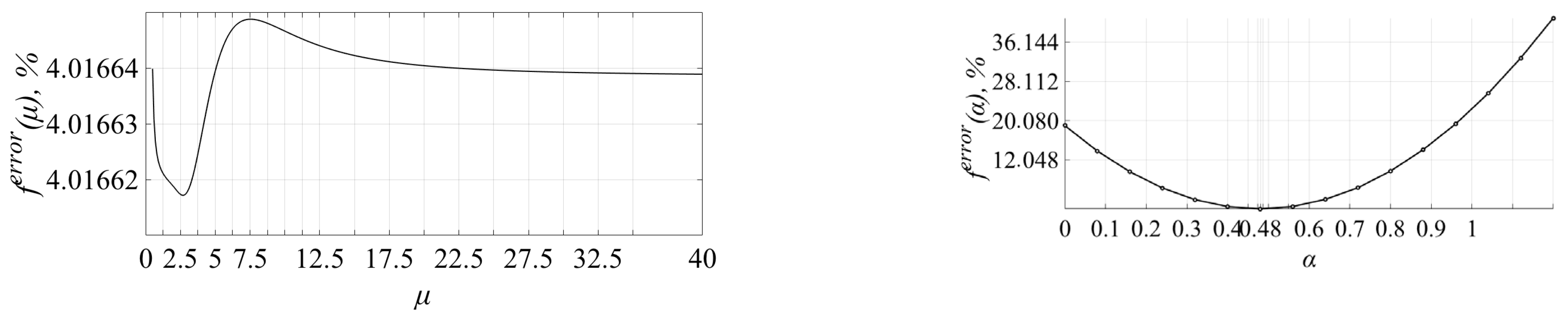
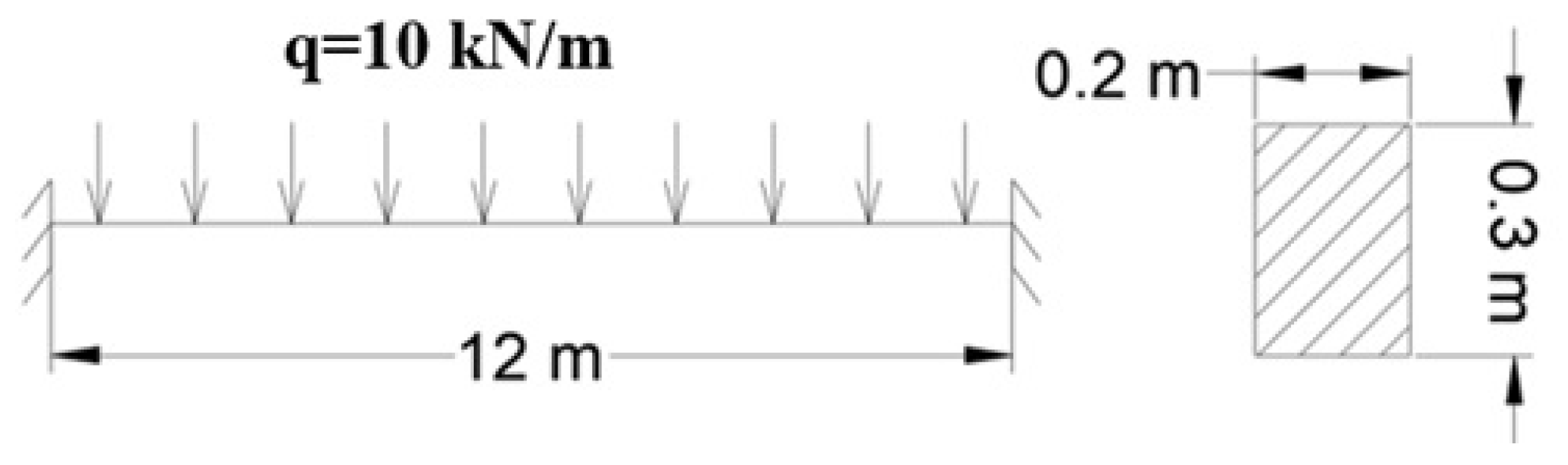
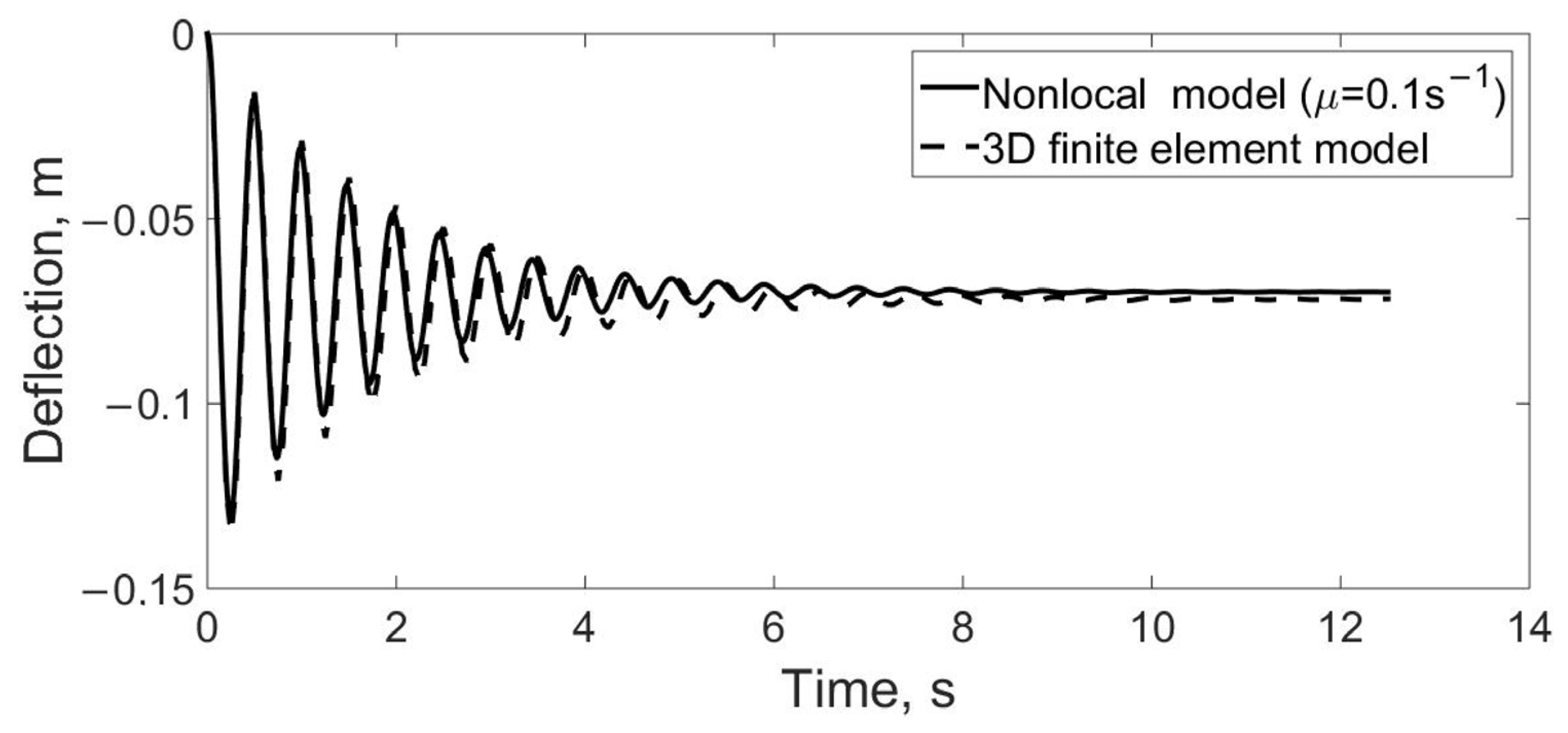
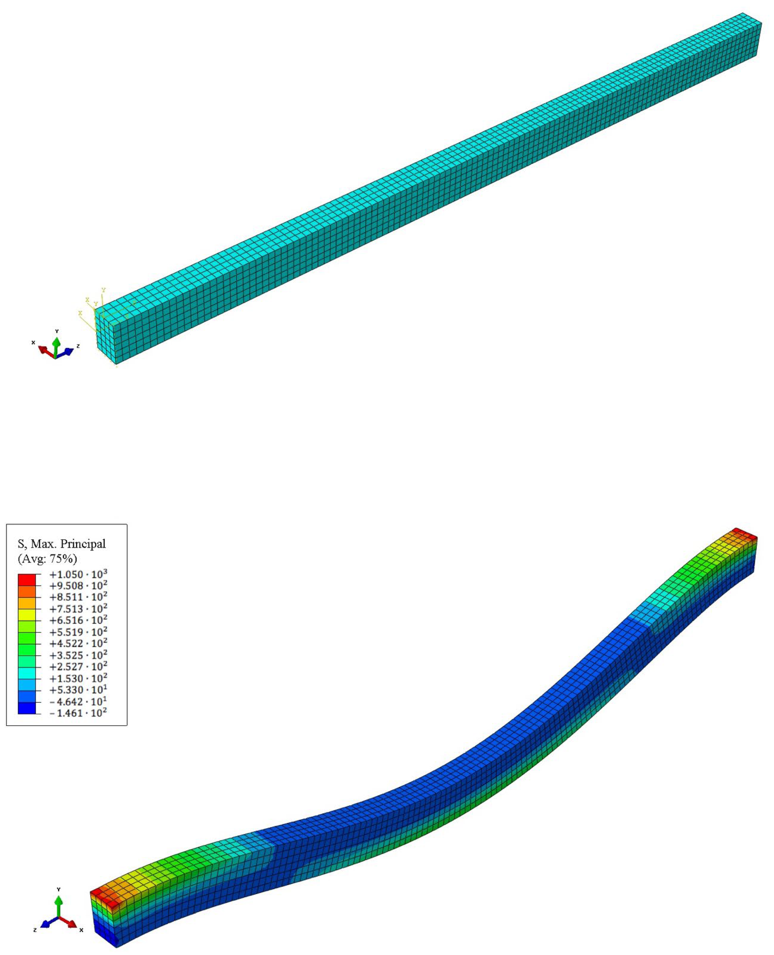
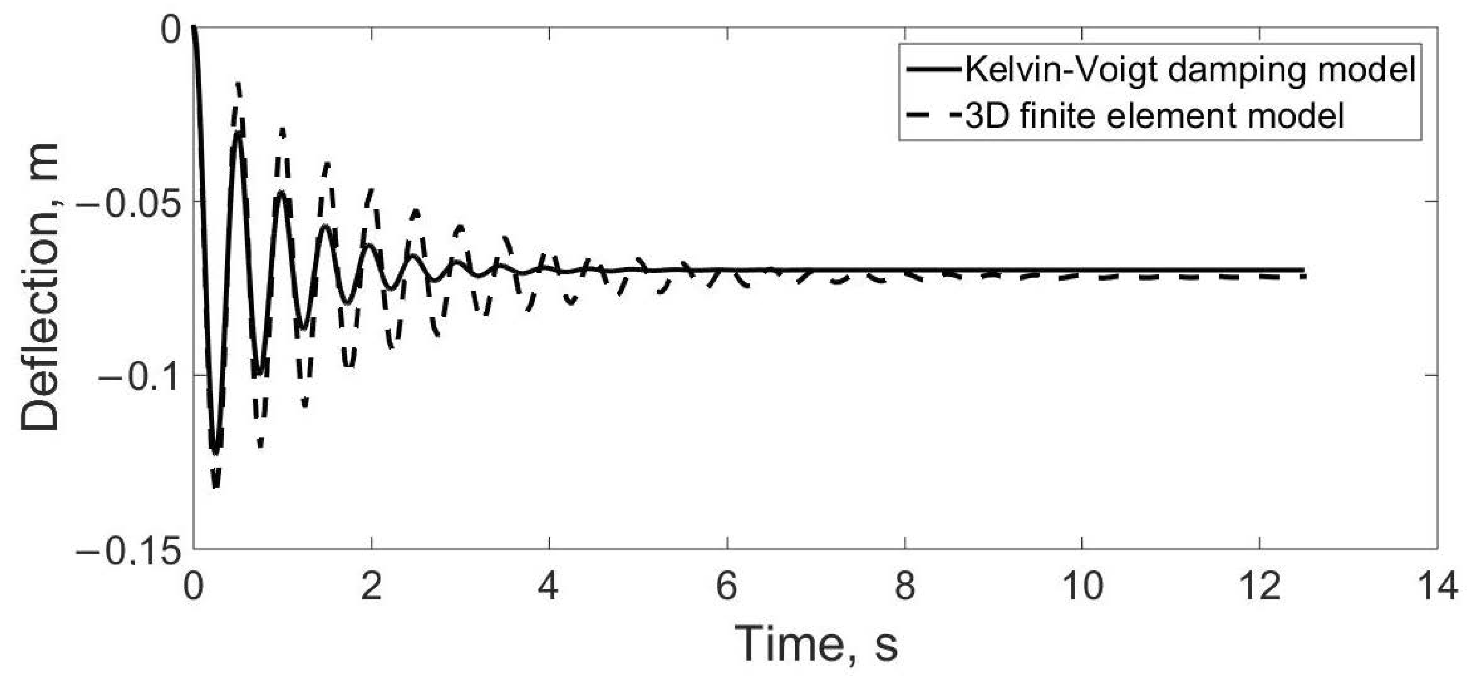
8. Numerical Example and Results for the Beam Model

The mathematical model of beam vibrations considering the nonlocal damping-with-memory was implemented in the MATLAB software package. In order to make this model to be applicable for practical use, it should be calibrated according to the results of experimental data.
The method for determining the parameter μ, describing the level of damping nonlocality of the beam material, based on the data of the numerical experiment via the least squares method is presented in Reference [65]. This technique was used to determine the influence distance for the damping-with-memory model in References [69,70]. For this purpose, a three-dimensional finite element model of the considered beam element was realized within the verified calculation software SIMULIA Abaqus CAE. The obtained data were imported into the MATLAB software package. Determination of the three parameters μ , α , M η , which control the nonlocal damping model, was implemented according to the rule of minimum error based on the least squares method (Figure 4):
100 % N · i = 1 N V ¯ e x p t i V ¯ m o d e l ( α , μ , M η , t i ) V ¯ e x p t i = f e r r o r ,
where N t = 251 is the number of time increments, V ¯ e x p t and V ¯ m o d e l ( α , μ , M η , t ) are, respectively, the displacement vector components obtained via numerical experiments and due to the nonlocal-in-time model.
As an example, let us consider the dynamic behavior of a composite beam shown in Figure 5, which was made of orthotropic thermoset vinyl ester class 1 GFRP, the properties of which were determined experimentally in References [74,75,76] and are given in Table 3. The beam is clamped at the ends and is subjected to instantly applied uniformly distributed load q = 10 kN/m.
The displacements of a middle span of the beam in time are shown in Figure 6. The solid line corresponds to the beam displacements obtained using the calibrated nonlocal model, and the dashed curve to those via a standard 3D model simulated in SIMULIA Abaqus (Figure 7).
In order to estimate the value of divergence between the results, the root-mean-square error σ e r r o r was calculated.
σ e r r o r = i = 1 N y i f i μ 2 N ,
where y i are the ordinates of the numerical experiment data, and f i ( μ ) are the ordinates of the results via the nonlocal-in-time damping model.
The root-mean-square error was 5.9% for the deflection at 20 s.
A comparison of the displacements of the middle node obtained using the classical (local in time) one-dimensional damping model based on the Voigt hypothesis with those obtained in SIMULIA Abaqus is shown in Figure 8. In this case, the relative root-mean-square error was 16.5%.
Instead of central differences (explicit scheme), the Newmark method (implicit scheme) could be utilized [69,70]. In this case, the nonlocal model becomes more stable and larger time increments could be implemented. The accuracy of the obtained results is almost the same in comparison to the central differences, but the time of one simulation of the vibration process is shortened more than twenty times [69].

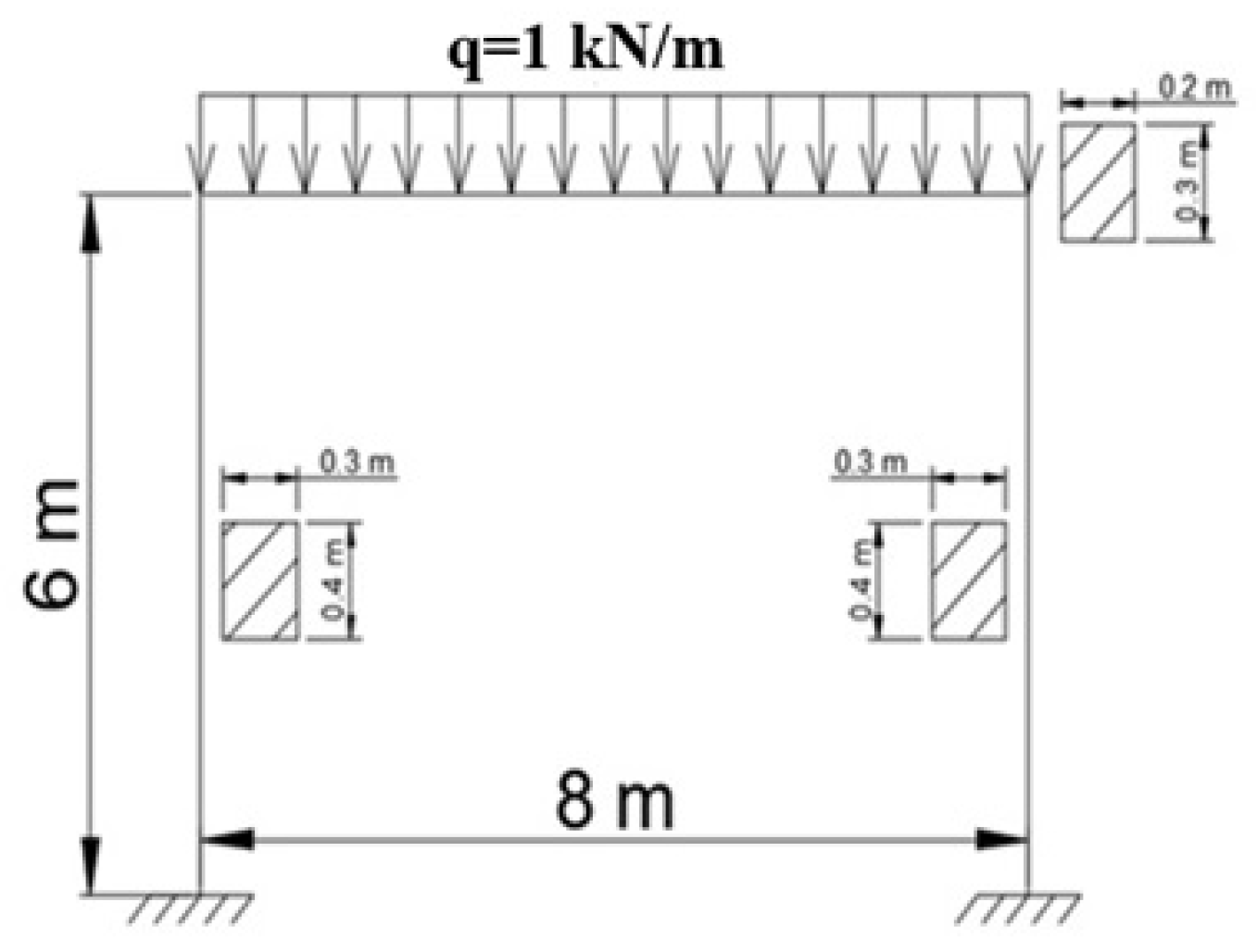
9. Modeling of Composite Frame Vibrations Considering Nonlocal-in-Time Damping Model

Let us show how the nonlocal-in-time damping model could be integrated into the FEA algorithm to study dynamic response of frame structures [77,78]. The equation of motion for the frame structure is similar to Equation (3), while the stiffness matrix for the 2D frame element has the following form [71]:
K i = E A l 0 0 E A l 0 0 0 12 E I l 3 6 E I l 2 0 12 E I l 3 6 E I l 2 0 6 E I l 2 4 E I l 0 6 E I l 2 2 E I l E A l 0 0 E A l 0 0 0 12 E I l 3 6 E I l 2 0 12 E I l 3 6 E I l 2 0 6 E I l 2 2 E I l 0 6 E I l 2 4 E I l .
The damping matrix could also be obtained according to the requirement of stationary state of the total energy of the vibrating system as was demonstrated earlier. The procedure for developing the damping matrix has been presented in detail in Reference [67]. Unlike the beam element, for the frame element, the axial displacement u should be taken into account. Then, energy dissipation could be written as follows:
Φ D i = 1 2 l χ ε ˙ a 2 A d z + 1 2 l A χ ε ˙ b 2 d A d z ,
where A is the frame element cross-section area, and ε ˙ a is the tension-induced axial strain rate.
Tension-induced axial strain is as follows [73]:
ε a = d u d z .
Then Equation (33) will take the form
Φ D i = 1 2 A χ l d u ˙ d z 2 d z + 1 2 I χ l d 2 v ˙ d z 2 2 d z .
Considering the linear shape function for the axial displacements N u = 1 ξ ξ relationship (35) could be transformed to:
Φ D i = 1 2 A χ 0 1 A u N u T A u N u u ˙ i 2 l d ξ + 1 2 I χ 0 1 A v N v T A v N v v ˙ i 2 l d ξ .
where u ˙ i = u ˙ 0 u ˙ l   is the vector of nodal velocities of axial displacements, A u = d l · d ξ , and u ˙ 0 and u ˙ l are velocities of the initial and terminal points of the i-th element.
Therefore, the damping matrix of the frame element D i could be written as follows:
D i = A χ 0 1 A u N u T A u N u l d ξ + I χ 0 1 A v N v T A v N v l d ξ ,
or
D i = χ A l 0 0 A l 0 0 0 12 I l 3 6 I l 2 0 12 I l 3 6 I l 2 0 6 I l 2 4 I l 0 6 I l 2 2 I l A l 0 0 A l 0 0 0 12 I l 3 6 I l 2 0 12 I l 3 6 I l 2 0 6 I l 2 2 I l 0 6 I l 2 4 I l .
In order to solve the equation of frame motion, the nonmodified Newmark method (an implicit scheme) could be used [71]. In this case, the first- and second-order time derivatives of the displacement vector V t (velocity and acceleration) entered into Equations (3) and (18) could be presented as follows:
V ˙ i + 1 = V i + 1 V i Δ t ,                     V ¨ i + 1 = 2 Δ t 2 V i + 1 V i V ˙ i Δ t V ¨ i .
Considering Relationships (39), Equation (18) is reduced to the following form:
M 2 Δ t 2 V i + 1 V i V ˙ i Δ t V ¨ i + D 1 Δ t j = 1 i + 1 G t i + 1 , τ j V ˙ j + K V i = F i .
Here G t i + 1 , τ j is the discrete analog of the G t τ kernel, which, for Error Function (20), is calculated as follows:
G t i + 1 , τ j = Δ t 2 μ π   e μ 2 t τ + Δ t 2 2 ,
where t = i + 1 Δ t , τ = j Δ t , and j = 1 , 2 , , i + 1 is the number of the time step, at which the displacement vector is calculated.
The Newmark scheme is implicit, so one needs to know V ˙ i + 1 to calculate the displacement vector. To solve this problem, the damping-with-memory term in Equation (40) should be divided into two parts, resulting in
M 2 Δ t 2 V i + 1 V i V ˙ i Δ t V ¨ i + β D + α D + K V i = F i ,
where one of two memory parts, α , is related to the i + 1 step, when the other, β , corresponds to all previous steps:
β = j = 1 i 2 μ π e μ 2 t j t j 1 2 V j V j 1 ,                                                                                                     α = 2 μ π e μ 2 t i + 1 t i 2 V i + 1 V i .
Equation (42) could be transformed into the computational scheme for the step-by-step calculation of V i + 1   using the vectors V i and V i 1 , which are calculated on the previous increments i and i 1
Z V i + 1 = F i + 1 + M V ¨ i + Q 1 V ˙ i + Q 2 V i + β D ,
where
Z = 2 Δ t 2 M + 1 Δ t α D + K ,               Q 1 = 2 Δ t M , Q 2 = 1 Δ t 2 Δ t M + α D .

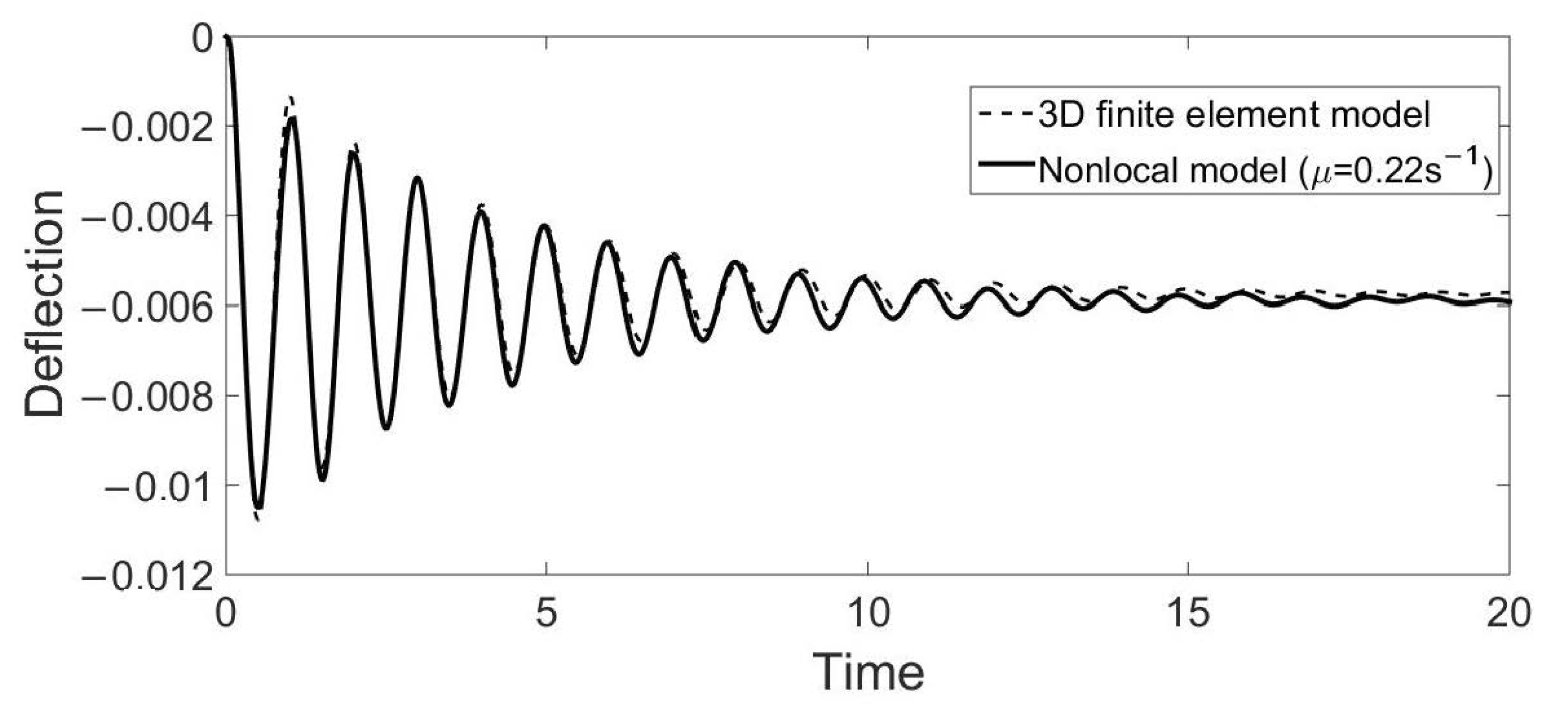
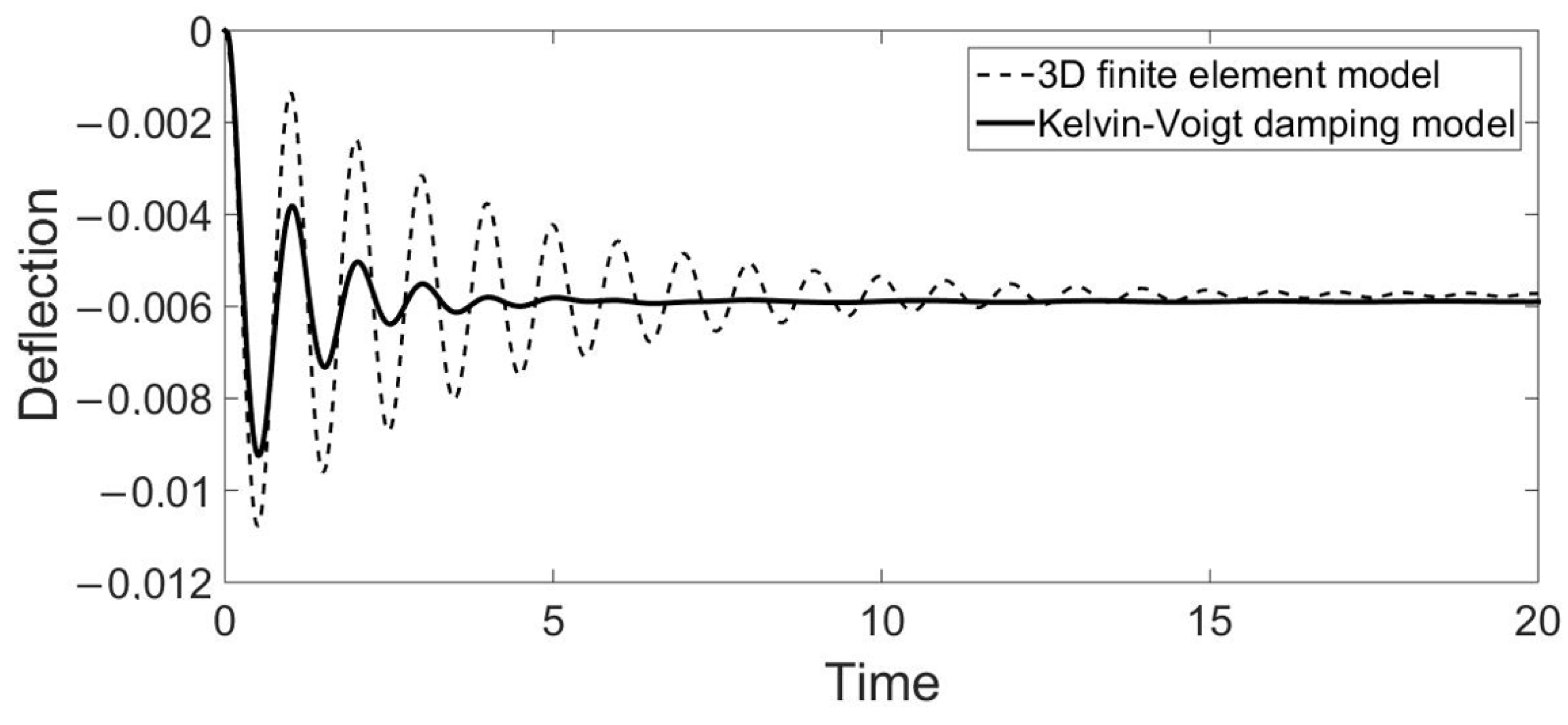
10. Numerical Results for the Frame Model

As a numerical example, the finite element model of a vibrating frame was implemented in the MATLAB software package. The frame geometry, boundary conditions, and loading are shown in Figure 9. The load is applied instantly.
The frame is made of the same material as the beam structure considered before.
For the first step of the simulated vibration process i = 1 , we assume V 1 = V ˙ 1 = V ¨ 1 = 0 as the initial conditions.
To determine the scale parameter for the considered structure, once again the computer simulation results obtained in SIMULIA Abaqus were used. The frame was modeled utilizing 3D-solid finite elements considering the orthotropic properties of the material. Using the least squares method, the magnitude of the parameter was calculated as μ = 0.22 , which points to a significant level of the nonlocal properties of the material. The deflection time history simulated by the calibrated nonlocal model in comparison with the results of 3D modeling via Abaqus is shown in Figure 10.
Even though the orthotropic properties of the material were not taken into account in the 2D-nonlocal-damping model of the frame, the results match the numerical experiment with satisfying accuracy. This is due to the fact that the nonlocal model could be flexibly controlled by its scale parameter μ . The difference between the results provided by the classical local-damping model and Abaqus data is shown in Figure 11.

11. Conclusions

From the review of damping models presented in this paper, it is evident that in comparison to local damping models, the nonlocal models allow one to obtain the main characteristics of the simulated vibration process in a more reliable and flexible way. The proposed models enable one to consider both internal and external damping at a time.
The enlarged flexibility makes it possible to use one-dimensional models of beam elements in the dynamic analysis of structures made of modern composite materials with orthotropic properties. The damping model with memory, which could be calibrated using the least-squares method, allows one to approximate the data of a numerical experiment with satisfactory accuracy.
The so-called nonlocal-in-time damping models are more easily integrated into the finite element method algorithm as compared with the nonlocal-by-coordinate damping models, what makes its application quite effective for solving different engineering problems.

Author Contributions

V.S.: Conceptualization, Formal analysis, Investigation, Methodology, Validation. M.S.: Conceptualization, Writing—review and editing, Supervision, Funding acquisition. E.B.: Methodology, Validation, Investigation, Writing—original draft. E.D.: Methodology, Validation, Visualization, Investigation. All authors have read and agreed to the published version of the manuscript.

Funding

This research was funded by grant No. 21-19-00634 from the Russian Science Foundation.

Data Availability Statement

All the data supporting the results are included in the manuscript.

Conflicts of Interest

The authors declare that they have no known competing financial interest or personal relationships that could have appeared to influence the work reported in this paper.

References

  1. Jones, R.M. Mechanics of Composite Materials, 2nd ed.; Taylor & Francis: Abingdon, UK, 1999. [Google Scholar]
  2. Pobedrja, B.E. Mechanics of Composite Materials; MGU: Moscow, Russia, 1984. (In Russian) [Google Scholar]
  3. Banks, H.T.; Inman, D.J. On damping mechanisms in beams. J. Appl. Mech. 1991, 58, 716–723. [Google Scholar] [CrossRef]
  4. Lei, Y.; Friswell, M.I.; Adhikari, S. A Galerkin method for distributed systems with non-local damping. Int. J. Solids Struct. 2006, 43, 3381–3400. [Google Scholar] [CrossRef] [Green Version]
  5. Postnikov, V.S. Internal Friction in Metals; Metallurgia: Moscow, Russia, 1974. (In Russian) [Google Scholar]
  6. Tseitlin, A.I.; Kusainov, A.A. Role of Internal Friction in Dynamic Analysis of Structures; Taylor & Francis: Abingdon, UK, 1999. [Google Scholar] [CrossRef]
  7. Sorokin, E.S. On the Theory of Internal Friction during Vibrations of Elastic Systems; Gosstroyizdat: Moscow, Russia, 1960. [Google Scholar]
  8. Shitikova, M.V. Fractional operator viscoelastic models in dynamic problems of mechanics of solids: A review. Mech. Solids 2022, 57, 1–33. [Google Scholar] [CrossRef]
  9. Shitikova, M.V.; Krusser, A.I. Models of viscoelastic materials: A review on historical development and formulation. Adv. Struct. Mater. 2022, 175, 285–326. [Google Scholar] [CrossRef]
  10. Tschoegl, N. The Phenomenological Theory of Linear Viscoelastic Behavior: An Introduction; Springer: Berlin, Germany, 1989. [Google Scholar]
  11. Ferry, J.D. Viscoelastic Properties of Polymers; John Wiley & Sons: Hoboken, NJ, USA, 1980. [Google Scholar]
  12. Fung, Y.C. Foundations of Solid Mechanics; Prentice-Hall: New York, NY, USA, 1965. [Google Scholar]
  13. Rabotnov, Y.N. Elements of Hereditary Solid Mechanics; Mir Publishers: Moscow, Russia, 1980. [Google Scholar]
  14. Voigt, W. Lehrbuch der Kristallphysik (mit Ausschluß der Kristalloptik); B.G. Teubner Verlag (Johnson Reprint Corporation): Stuttgart, Germany, 1966. [Google Scholar]
  15. Maxwell, J.C. On the dynamical theory of gases. Phil. Trans. R. Soc. 1867, 49, 49–88. [Google Scholar] [CrossRef]
  16. Nashif, A.; Jones, D.; Henderson, J. Vibration Damping; Wiley: Hoboken, NJ, USA, 1984. [Google Scholar]
  17. Adhikari, S. Damping Models for Structural Vibration. Ph.D. Thesis, Trinity College, Cambridge, UK, 2000. [Google Scholar]
  18. Adhikari, S.; Woodhouse, J. Identification of damping. Part 2: Non-viscous damping. J. Sound Vib. 2001, 243, 63–88. [Google Scholar] [CrossRef] [Green Version]
  19. Eremeyev, V.A.; Lurie, S.A.; Solyaev, Y.O.; dell’Isola, F. On the well posedness of static boundary value problem within the linear dilatational strain gradient elasticity. Z. Angew. Math. Phys. 2020, 71, 182. [Google Scholar] [CrossRef]
  20. Rossikhin, Y.A.; Shitikova, M.V. Application of fractional calculus for dynamic problems of solid mechanics: Novel trends and recent results. Appl. Mech. Rev. 2010, 63, 010801. [Google Scholar] [CrossRef]
  21. Rossikhin, Y.A.; Shitikova, M.V. Fractional operator models of viscoelasticity. In Encyclopedia of Continuum Mechanics; Altenbach, H., Öchsner, A., Eds.; Springer: Berlin/Heidelberg, Germany, 2020; Volume 2, pp. 971–982. [Google Scholar] [CrossRef]
  22. Rossikhin, Y.A.; Shitikova, M.V. Fractional calculus in structural mechanics. In Handbook of Fractional Calculus with Applications; Applications in Engineering, Life and Social Sciences, Part A; Baleanu, D., Lopes, A.M., Eds.; De Gruyter: Berlin, Germany, 2019; Volume 7, pp. 159–192. [Google Scholar] [CrossRef]
  23. Bažant, Z.P.; Jirásek, M. Nonlocal integral formulations of plasticity and damage: Survey of progress. J. Eng. Mech. 2002, 128, 1119–1149. [Google Scholar] [CrossRef] [Green Version]
  24. Di Paola, M.; Failla, G.; Pirrotta, A.; Sofi, A.; Zingales, M. The mechanically based non-local elasticity: An overview of main results and future challenges. Phil. Trans. R. Soc. A 2013, 371, 20120433. [Google Scholar] [CrossRef] [PubMed] [Green Version]
  25. Zorica, D. Hereditariness and non-locality in wave propagation modelling. Theor. Appl. Mech. 2020, 47, 19–31. [Google Scholar] [CrossRef]
  26. Rahimi, Z.; Rezazadeh, G.; Sumelka, W. A non-local fractional stress–strain gradient theory. Int. J. Mech. Mat. Des. 2020, 16, 265–278. [Google Scholar] [CrossRef]
  27. Alotta, G.; Failla, G.; Zingales, M. Finite-element formulation of a nonlocal hereditary fractional-order Timoshenko beam. J. Eng. Mech. 2017, 143, D4015001. [Google Scholar] [CrossRef]
  28. Flügge, W. Viscoelasticity, 2nd ed.; Springer: Berlin/Heidelberg, Germany, 1975. [Google Scholar]
  29. Eringen, A.C.; Edelen, D.G.B. Nonlocal elasticity. Int. J. Eng. Sci. 1972, 10, 233–248. [Google Scholar] [CrossRef]
  30. Pisano, A.A.; Fuschi, P. Closed form solution for non-local elastics bar in tension. Int. J. Solids Struct. 2003, 40, 13–23. [Google Scholar] [CrossRef]
  31. Polizzotto, C. Nonlocal elasticity and related variational principles. Int. J. Solids Struct. 2001, 38, 42–43. [Google Scholar] [CrossRef]
  32. Fuschi, P.; Pisano, A.A.; Polizzotto, C. Size effects of small-scale beams addressed with a strain-difference based nonlocal elasticity theory. Int. J. Mech. Sci. 2019, 151, 661–671. [Google Scholar] [CrossRef]
  33. Ahmadi, G. Linear theory of non-local viscoelasticity. Int. J. Non-Linear Mech. 1975, 10, 253–258. [Google Scholar] [CrossRef]
  34. Barretta, R.; Marotti de Sciarra, F.; Pinnola, F.P. On the nonlocal bending problem with fractional hereditariness. Meccanica 2021, 57, 807–820. [Google Scholar] [CrossRef]
  35. Boltzmann, L. Zur Theorie der elastischen Nachwirkung. Ann. Phys. Chem. 1876, 7, 624–657. [Google Scholar]
  36. Volterra, V. Leçons sur les Fonctions de Lignes; Cauthier-Villard: Paris, France, 1913. [Google Scholar]
  37. Rabotnov, Y.N. Equilibrium of an elastic medium with after-effect. Prikl. Mat. Meh. 1948, 12, 81–91. English Trans.: Fract. Calc. Appl. Anal. 2014, 17, 684–696(In Russian) [Google Scholar] [CrossRef]
  38. Rabotnov, Y.N. Creep Problems in Structural Members; Nauka: Moscow, Russia, 1966; English Edition by North-Holland: Amsterdam, Holland, 1969. (In Russian) [Google Scholar]
  39. Kunin, I.A. Theory of Elastic Media with Microstructure. In The Nonlocal Theory of Elasticity; Nauka: Moscow, Russia, 1975; English Edition: Elastic Media with Microstructure I: One-Dimensional Models. Springer Series in Solid-State Sciences 26; Springer: Heidelberg, Germany, 1982; (In Russian). [Google Scholar] [CrossRef]
  40. Karličić, D.; Cajić, M.; Murmu, T.; Adhikari, S. Nonlocal longitudinal vibration of viscoelastic coupled double-nanorod systems. Eur. J. Mech. A/Solids 2015, 49, 183–196. [Google Scholar] [CrossRef]
  41. Karličić, D.; Cajić, M.; Adhikari, S.; Kozic, P.; Murmu, T. Vibrating nonlocal multi-nanoplate system under inplane magnetic field. Eur. J. Mech. A/Solids 2017, 64, 29–45. [Google Scholar] [CrossRef] [Green Version]
  42. Ghavanloo, E.; Shaat, M. General nonlocal Kelvin–Voigt viscoelasticity: Application to wave propagation in viscoelastic media. Acta Mech. 2022, 233, 57–67. [Google Scholar] [CrossRef]
  43. Potapov, V.D. Stability via nonlocal continuum mechanics. Int. J. Solids Struct. 2013, 50, 637–641. [Google Scholar] [CrossRef]
  44. Potapov, V.D. On the stability of a rod under deterministic and stochastic loading with allowance for nonlocal elasticity and nonlocal material damping. J. Mach. Manuf. Reliab. 2015, 44, 6–13. [Google Scholar] [CrossRef]
  45. Russell, D.L. On mathematical models for the elastic beam with frequency-proportional damping. In Control and Estimation in Distributed Parameter Systems; Banks, H.T., Ed.; SIAM: Philadelphia, PA, USA, 1992; pp. 125–169. [Google Scholar] [CrossRef]
  46. Adhikari, S.; Friswell, M.I.; Lei, Y. Modal analysis of nonviscously damped beams. J. Appl. Mech. 2007, 74, 1026–1030. [Google Scholar] [CrossRef]
  47. Friswell, M.I.; Adhikari, S.; Lei, Y. Non-local finite element analysis of damped beams. Int. J. Solids Struct. 2007, 44, 7564–7576. [Google Scholar] [CrossRef]
  48. Friswell, M.I.; Adhikari, S.; Lei, Y. Vibration analysis of beams with non-local foundations using the finite element method. Int. J. Num. Meth. Eng. 2007, 71, 1365–1386. [Google Scholar] [CrossRef]
  49. Lei, Y.; Murmu, T.; Adhikari, S.; Friswell, M.I. Dynamic characteristics of damped viscoelastic nonlocal Euler–Bernoulli beams. Eur. J. Mech. A Solids 2013, 42, 125–136. [Google Scholar] [CrossRef]
  50. Lei, Y.; Adhikari, S.A.; Friswell, M.I. Vibration of nonlocal Kelvin–Voigt viscoelastic damped Timoshenko beams. Int. J. Eng. Sci. 2013, 66–67, 1–13. [Google Scholar] [CrossRef]
  51. Adhikari, S.; Karličić, D.; Liu, X. Dynamic stiffness of nonlocal damped nano-beams on elastic foundation. Eur. J. Mech. A Solids 2021, 86, 104144. [Google Scholar] [CrossRef]
  52. Gonzalez-Lopez, S.; Fernandez-Saez, J. Vibrations in Euler–Bernoulli beams treated with non-local damping patches. Comput. Struct. 2012, 108–109, 125–134. [Google Scholar] [CrossRef]
  53. Puthanpurayil, A.M.; Carr, A.J.; Dhakal, R.P. Application of nonlocal elasticity continuum damping models in nonlinear dynamic analysis. Bull. Earthq. Eng. 2018, 16, 6269–6297. [Google Scholar] [CrossRef]
  54. Cavalcanti, M.M.; Domingos Cavalcanti, V.N.; Ma, T.F. Exponential decay of the viscoelastic Euler-Bernoulli equation with a nonlocal dissipation in general domains. Diff. Integral Equ. 2004, 17, 495–510. [Google Scholar] [CrossRef]
  55. Jorge Silva, M.A.; Narciso, V. Long-time behavior for a plate equation with nonlocal weak damping. Diff. Integral Equ. 2014, 27, 931–948. [Google Scholar]
  56. Jorge Silva, M.A.; Narciso, V. Attractors and their properties for a class of nonlocal extensible beams. Discret. Contin. Dyn. Syst. 2015, 35, 985–1008. [Google Scholar] [CrossRef]
  57. Jorge Silva, M.A.; Narciso, V. Long-time dynamics for a class of extensible beams with nonlocal nonlinear damping. Evol. Equ. Control Theory 2017, 6, 437–470. [Google Scholar] [CrossRef] [Green Version]
  58. Jorge Silva, M.A.; Narciso, V.; Vicente, A. On a beam model related to flight structures with nonlocal energy damping. Discret. Contin. Dyn. Syst. Ser. B 2019, 24, 3281–3298. [Google Scholar] [CrossRef] [Green Version]
  59. Gomes Tavares, E.H.; Jorge Silva, M.A.; Narciso, V. Long-time dynamics of Balakrishnan–Taylor extensible beams. J. Dyn. Diff. Equ. 2020, 32, 1157–1175. [Google Scholar] [CrossRef]
  60. Zhao, C.; Meng, F.; Zhong, C. The well-posedness and attractor on an extensible beam equation with nonlocal weak damping. Discret. Contin. Dyn. Syst. Ser. B 2023, 28, 2884–2910. [Google Scholar] [CrossRef]
  61. Potapov, V.D. On the stability of columns under stochastic loading taking into account nonlocal damping. J. Mach. Manuf. Reliab. 2012, 41, 284–290. [Google Scholar] [CrossRef]
  62. Potapov, V.D. Stability of a flat arch subjected to deterministic and stochastic loads taking into account nonlocal damping. J. Mach. Manuf. Reliab. 2013, 42, 450–456. [Google Scholar] [CrossRef]
  63. Potapov, V.D.; Shepitko, E.S. Computer modeling of nonlinear system vibrations with allowance for nonlocal damping. Int. J. Comput. Civ. Struct. Eng. 2018, 14, 137–144. [Google Scholar] [CrossRef] [Green Version]
  64. Fyodorov, V.S.; Sidorov, V.N.; Shepitko, E.S. Nonlocal damping consideration for the computer modelling of linear and nonlinear systems vibrations under the stochastic loads. IOP Conf. Ser. Mat. Sci. Eng. 2018, 456, 012040. [Google Scholar] [CrossRef]
  65. Shepitko, E.S.; Sidorov, V.N. Defining of nonlocal damping model parameters based on composite beam dynamic behavior numerical simulation results. IOP Conf. Ser. Mat. Sci. Eng. 2019, 675, 012056. [Google Scholar] [CrossRef] [Green Version]
  66. Fyodorov, V.S.; Sidorov, V.N.; Shepitko, E.S. Computer simulation of composite beams dynamic behavior. Mat. Sci. Forum 2020, 974, 687–692. [Google Scholar] [CrossRef]
  67. Sidorov, V.N.; Badina, E.S.; Detina, E.P. Nonlocal in time model of material damping in composite structural elements dynamic analysis. Int. J. Comput. Civ. Struct. Eng. 2021, 17, 14–21. [Google Scholar] [CrossRef]
  68. Sidorov, V.N.; Badina, E.S. Nonlocal numerical damping model in beam dynamics simulation. Lect. Notes Civ. Eng. 2022, 189, 357–363. [Google Scholar] [CrossRef]
  69. Sidorov, V.N.; Badina, E.S.; Detina, E.P. Modified Newmark method for the dynamic analysis of composite structural elements considering damping with memory. Mech. Compos. Mat. Struct. 2022, 28, 98–111. [Google Scholar] [CrossRef]
  70. Sidorov, V.N.; Badina, E.S.; Detina, E.P. A modified implicit scheme for the numerical dynamic analysis of beam elements considering nonlocal in time internal damping. Lect. Notes Civ. Eng. 2023, 308, 226–234. [Google Scholar] [CrossRef]
  71. Bathe, K.J.; Wilson, E.L. Numerical Methods in Finite Element Analysis; Prentice Hall: New York, NY, USA, 1976. [Google Scholar]
  72. Alexandrov, A.V.; Potapov, V.D.; Zylev, V.B. Structural Mechanics. Book 2. Dynamics and Stability of the Elastic Systems; Vysshaya shkola: Moscow, Russia, 2008. (In Russian) [Google Scholar]
  73. Sidorov, V.N. Mechanics of Materials; Architecture-S: Moscow, Russia, 2013. [Google Scholar]
  74. Landherr, J.C. Dynamic Analysis of a FRP Deployable Box Beam. Master’s Thesis, Queen’s University, Kingston, ON, Canada, 2008. [Google Scholar]
  75. Lim, R.A. Structural Monitoring of a 10 m Fiber Reinforced Polymer Bridge Subjected to Severe Damage. Master’s Thesis, Queen’s University, Kingston, ON, Canada, 2016. [Google Scholar]
  76. Xie, A. Development of an FRP Deployable Bridge. Master’s Thesis, Royal Military College of Canada, Kingston, ON, Canada, 2007. [Google Scholar]
  77. Sidorov, V.N.; Badjina, E.S.; Detina, E.P.; Shitikova, M.V. Numerical simulation of the frame structure dynamic behavior by the application of the nonlocal in time damping model. In Proceedings of the 1st International Conference on Mathematical Modelling in Mechanics and Engineering, Belgrade, Serbia, 8–10 September 2022. [Google Scholar]
  78. Sidorov, V.N.; Badina, E.S.; Detina, E.P. Computer simulation of the composite frame structures vibrations considering nonlocal in time internal damping. Mech. Compos. Mat. Struct. 2022, 28, 543–552. [Google Scholar]
Figure 1. Dependence of the nonlocality level on the parameter μ .
Axioms 12 00676 g001
Figure 2. A scheme of the elements of the acceleration vector V ¯ ¨ t within the analyzed time steps t i 1   a n d   t i + 1 .
Axioms 12 00676 g002
Figure 3. Unlimited kernel function G j i ( M η = T ) and kernel function G k i limited with the memory interval M η = 0.06 s.
Axioms 12 00676 g003
Figure 4. Error variation f e r r o r [ % ] depending on μ 0.25 s   a n d   α ( 0.1 ) .
Axioms 12 00676 g004
Figure 5. Scheme of the beam.
Axioms 12 00676 g005
Figure 6. Comparison of the results obtained using the calibrated nonlocal model with the data of the numerical experiment.
Axioms 12 00676 g006
Figure 7. Beam behavior simulation in SIMULIA Abaqus.
Axioms 12 00676 g007
Figure 8. Comparison of the numerical experiment data with the results obtained using the classical internal friction model.
Axioms 12 00676 g008
Figure 9. Scheme of the frame.
Axioms 12 00676 g009
Figure 10. Comparison of the results obtained by the calibrated nonlocal model with those by the 3D-numerical simulation.
Axioms 12 00676 g010
Figure 11. Comparison of the results obtained by the classical local model with those by the 3D numerical simulation.
Axioms 12 00676 g011
Table 1. Basic models of internal damping.
Basic Classical Models of Damping due to Internal Friction
Kelvin–Voigt model σ = E ε + t κ ε ˙ [3,8,50,63,66]
Sorokin’s complex stiffness model σ = 1 + i γ E ε [3]
Nonlocal models of damping due to internal friction
Internal friction model nonlocal-in-spatial coordinate x σ x , t = E ε x , t + χ 0 l C x θ ε ˙ θ , t d θ [3,50,63,64,65,66]
Internal friction model nonlocal-in-time t σ x , t = E ε x , t + χ t G t τ ε ˙ x , τ d τ [3,67,68,69,70]
Table 2. Kernel functions used in nonlocal damping models.
Kernel Functions for Nonlocal-in-Space Damping Models
Exponential kernel function C x θ = μ 2     e μ x θ [50,63,64,65,66]
Error kernel function C x θ = μ 2 π   e μ 2 ( x θ ) 2 2 [3,50,53]
Hat kernel function C x θ = 1 l 0 ,           for   x θ l 0 2 0 ,                       otherwise   [50]
Triangular kernel function C x θ = 1 l 0 1 x θ l 0 ,   for   x θ l 0 0 ,                               otherwise [50]
Kernel functions for nonlocal-in-time damping models
Exponential kernel function G v t τ = μ e μ t τ [67]
Error kernel function G ν t τ = 2 μ π e μ 2 t τ 2 [67,69,70,71]
Table 3. Properties of thermosetting vinyl ester fiberglass 1FRP [74,75,76].
Young’s modulus in the longitudinal direction Elong17.2 GPa
Young’s modulus in the transverse direction Etrans12.2 GPa
Poisson’s ratio in the longitudinal direction μlong0.32
Poisson’s ratio in the transverse direction μtrans0.15
density of the material ρ1900 kg/m3
Damping coefficient (critical fraction)0.042
Disclaimer/Publisher’s Note: The statements, opinions and data contained in all publications are solely those of the individual author(s) and contributor(s) and not of MDPI and/or the editor(s). MDPI and/or the editor(s) disclaim responsibility for any injury to people or property resulting from any ideas, methods, instructions or products referred to in the content.

