1. Introduction
The thermoelasticity theory integrates the concepts of elasticity and heat transfer. It is concerned with how heat affects the deformation of elastic media and how this deformation, in turn, affects the thermal state of the medium under study. When the temporal variance of a heat source in a medium or the temporal variance of thermal boundary conditions over a medium contrast with the oscillation features of the structure, thermal stress is generated. When it comes to describing the physical state of an elastic material as it relates to temperature, the thermoelasticity theory provides a more accurate description than elasticity does. Recently, there has been a lot of interest in the possible applications of the thermoelasticity theory in geophysics, plasma physics, and related topics, specifically in consideration of the interactions between magnetic fields, non-thermal forces, and rotation. Magnetic fields, rotation, and huge temperature gradients are other factors that need to be considered during the construction and operation of equipment, especially in nuclear research. Scientists apply their knowledge of thermoelasticity to develop materials and objects that can withstand wide temperature fluctuations without cracking.
Yadav and Singh [
1] investigated thermoelastic and electromagnetic plane waves. Augustine Lgwebuike et al. [
2] looked at the behavior of plane waves in thermoelastic and magneto-thermoelastic media. Verma and Maiti recently solved the thermal shock problem [
3]. In [
4], Choudhury investigated the issue of wave propagation in a generalized thermoelastic medium that was both spinning and micropolar. Singh and Chakraborty [
5] investigated the reflected plane magneto-thermoelastic wave at a solid half-space boundary, while the system was subjected to initial stress. Aboueregal and Sedighi [
6] investigated the thermoviscoelasticity of an unbounded annular cylinder to determine the transition temperature and stresses caused by thermal expansion. The inner and outer surfaces are frictionless and free of thermal insulation, while the inner surface is heated by thermal shock. Zhu et al. [
7] investigated the behavior of a thermoelastic half-steady-state plane in the presence of voids, subjected to a thermal source, and under the influence of a harmonic force. Abouelregal and Abo-dahab [
8] considered the generalized form of the equations of generalized thermoelasticity for a heterogeneous isotropic flexible half-space solid with a mode-I fracture issue on its surface caused by rotation. Within the Lord–Shulman theory of thermoelasticity framework, Yadav [
9] investigated the phenomenon of the propagation of plane waves in a rotating magneto-thermoelastic half-space with diffusion. After formulating the governing equations for a certain plane and solving them, one obtains the velocity equation, which reveals the presence of four plane waves linked together.
When three different types of shot Vanadium titanomagnetite (VTM) pellets were discharged, Shi et al. [
10] examined reduction behaviors and mechanisms. Because of their reduction property, vanadium titanomagnetite (VTM) pellets are a crucial for the rotary kiln-electric furnace method. The exceptional function of Zn in improving the thermoelectric performance of Ga-doped PbTe was described by Luo et al. [
11]. Zn is shown to enhance the electronic transport characteristics and reduce the lattice thermal conductivity of Ga-doped PbTe, achieving a maximum ZT value of 1.55 at 723 K and a record high ZTavg~1.26 across the temperature range of 400–873 K. Because of its high entropy, Wang et al. [
12] improved the thermophysical properties of rare earth tantalate ceramics.
Najibi and Wang [
13] used quadratic Lagrangian shape functions to design a graded finite element analysis algorithm to resolve the axisymmetric 2D hyperbolic heat transfer problem in a finite hollow cylinder composed of functionally graded solids. For newly suggested functionally graded porosity (FGP) media, Najibi and Shojaeefard [
14] conducted the numerical analysis of heat transfer. The responses of Fourier, Cattaneo–Vernotte (C-V), dual-phase lag (DPL), and time-fractional heat transfer for a porous solid–gas medium were compared with the experimental findings of various flux pulse durations. Through the use of the Lord–Shulman theory, Jani and Kiani [
15] investigated the response of a hollow piezoelectric disc. By reducing the governing equations of the general state to those of the plane stress state, we are able to obtain governing equations for the system. For the thermo-viscoelasticity issue of a hollow sphere, Javani et al. [
16] presented a unified formulation that incorporates the LS, GL, and GN theories, as well as the impacts of viscosity. The Kelvin–Voigt viscosity concept is used to define the characteristics of materials. Additional research on generalized thermoelasticity for functionally graded materials may be found in [
17].
Biot’s traditional theory of thermoelasticity [
18] contrasts with many representations of thermal resistance, which use the equivalent thermodynamic equation and predict an infinite velocity of heat transfer within the medium. That is why a variety of generalized thermoelastic models with multiple applications have emerged to solve such problems. To remedy the shortcomings found in the Biot theory [
18], Lord and Shulman [
19] and Green and Lindsay [
20] improved it by including the idea of the relaxation time coefficient in the heat transfer vector based on the idea of Cattaneo–Vernotte [
21,
22,
23]. Using an expanded thermodynamics system, Sarkar and Singh [
24] provided the constitutive modeling of a new generalized thermoelasticity framework by incorporating a strain-rate term coupled with a relaxation time coefficient into the Lord–Shulman (LS) thermoelasticity theory. Sherief et al. [
25] considered a two-dimensional axisymmetric problem involving an infinite body. Within the body, there is an infinite cylinder made of different materials and harboring a variable heat source. The mathematical model for the transmission of waves in an extended thermoelastic, multiple-layered composite hollow cylinder was developed by Mahesh and Selvamani [
26]. This cylinder has a visco-thermoelastic layer on the inside and a linear flexible material on the outside, and the layers are held together with fasteners. Kumar et al. [
27] discovered how particle Rayleigh wave motion, attenuation, and phase velocity change in a generalized, nonlocalized thermal medium. Yang et al. [
28] established a technique to address issues combining coupled mechanical and thermal movements and to study the propagation properties of thermoelastic waves produced by point sources in a three-dimensional, multilayered half-space. Malik et al. [
29] were interested in wave transmission with diffusion over the boundary of two different nonlocally modified thermoelastic substances. The impact of the thermoelastic medium on wave propagation can be shown once the mathematical issue has been formulated.
Green and Naghdi [
30,
31,
32] have also contributed a theoretical model to this field by making sufficient basic adjustments to the constitutive equations to allow the analysis of a considerably broader class of heat flow issues. The method used by the authors of [
30,
31,
32] involves entropy balancing. They initially proposed this entropy equilibrium in [
33]. The common practices in thermodynamics typically include using an inequality like Clausius–Duhem or a related inequality.
Since its introduction, the Moore–Gibson–Thompson (MGT) equation has been the subject of many research studies. Since high-intensity ultrasound has many practical uses in medicine and industry, such as lithotripsy, heat treatment, ultrasonic cleaning, etc., there has been a great number of studies in this field. In the field of thermoelasticity, Quintanilla [
34] introduced a new model of heat transfer by including the MGT equation in the heat conduction equation. In fact, by adding a relaxation coefficient to the Green–Naghdi type III model, this new equation for thermal conductivity can be derived. In fact, this equation can be obtained after the introduction of a relaxation parameter to the Green–Naghdi type III model. Abouelregal et al. presented numerous new thermoelasticity equation systems and numerous applications in this context in response to Quintanilla’s proposal [
35,
36,
37,
38,
39,
40,
41]. This modified model has been used to investigate the difficulties of fluid mechanics and the thermal and mechanical behaviors of different engineering structures [
42,
43,
44,
45,
46,
47,
48,
49].
Many researchers have studied coupling between the modified Fourier law of thermal conductivity and different systems, and many results have been presented. Although many authors have studied the effect of electromagnetism, only a few researchers have taken into account the effects of modified Ohm’s and Fourier’s laws. In this paper, we extend Ohm’s law by incorporating two new terms: one accounts for the temperature gradient (also known as the Seebeck influence), and the other considers the cross-product of velocity and the initial magnetic field. Not only that, but Fourier’s law of thermal conductivity has also been modified for the Green and Naghdi model of the third kind [
31] to include the factor of relaxation time. One of the advantages of this new model is that the relaxation time coefficient plays an important role in reducing the propagation of heat waves.
As a direct application to the proposed model, a two-dimensional problem was investigated for a homogeneous, isotropic, elastic thermal body in the form of half an area when the boundaries are stress free and subject to time-dependent variable thermal shocks. A magnetic field of constant intensity is also present around the medium’s free surface. In order to fully solve the problem, a normal model analysis method was used. The numerical results are analyzed and discussed using graphical representations of the studied physical fields. Finally, the results of this investigation were compared with those obtained in the previous literature in the presence and absence of relaxation time.
2. Mathematical Model and Basic Equations
It is taken into account that the studied thermoelastic medium rotates with a constant angular velocity,
, so that the direction of the axis of rotation is indicated by a unit vector,
. As a result, there are two additional terms in the equation for motion due to an accelerated reference frame: (1) centripetal acceleration,
, due to time-independent motion and (2) Coriolis acceleration,
, due to the motion of the reference frame [
50]. The form of the differential equations for generalized electromagnetic thermoelasticity is based on the MGT thermal conductivity theory.
where
is the stress tensor,
is the strain tensor,
signifies the density,
,
is the absolute temperature,
denotes the displacement vector,
is the identity tensor,
denotes the transpose of a matrix,
is the body force vector,
is the reference temperature determined, so that
,
,
is the thermal expansion coefficient and Lame’s constants are denoted by the notations,
and
.
Applying a magnetic field of constant strength,
, generates an induced magnetic field,
, and an induced electric field,
, inside the medium. Electromagnetism has governing equations that may be derived from Maxwell’s magnetic and electric field equations. The following form can offer simpler equations for an electrically and thermally conductive homogeneous elastic material [
50]:
In this equation,
denotes the current density vector,
measures the magnetic permeability,
and
correspond to the electric and magnetic induction vectors, respectively [
43],
provides the electric permeability, and
illustrates the electric charge density. A modified version of Ohm’s Law for use with thermoelastic materials is stated as follows [
51]:
where
is the Ohm’s law modification coefficient and
is the electrical conductivity at room temperature.
can be used to represent the coefficient connecting the temperature difference to the resulting electric current, where
is called the Seebeck coefficient (thermoelectric sensitivity). This induced thermoelectric voltage is induced when there is a temperature difference between the two sides of the material.
The improved GN-III system led to the proposal of a new form of Fourier’s law as per the following formula [
31]
where
represents the direction and magnitudes of the heat flow vector,
denotes the thermal conductivity, and
indicates the rate of thermal conductivity. Also, the variable,
, designates the thermal displacement and is related to the distribution of the heat by the relationship,
.
The equation that can be used to describe energy is as follows:
where
stands for the specific heat,
stands for the heat supply, and
represents the cubical dilatation that is defined as:
The revised version of the heat equation that Quintanilla developed can be seen in the following equation [
34]
where
is the relaxation time coefficient.
It is possible to combine Equations (10) and (12) to produce the modified MGT heat transfer equation, which is defined as [
36,
38]
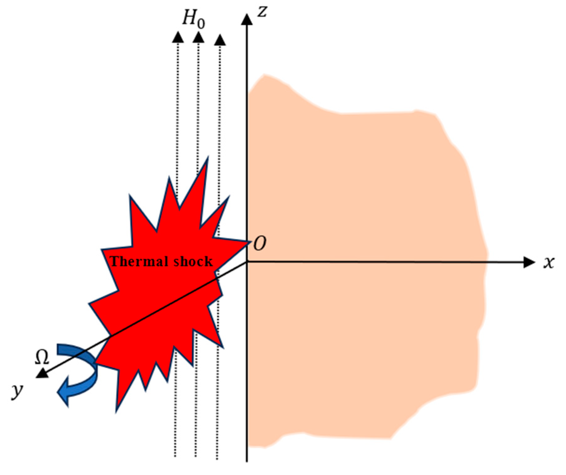
3. Problem Formulation
In this analysis, a homogeneous, isotropic, generalized thermoelastic semi-infinite solid occupying the area,
, is considered. It is assumed that the border,
, is unconstrained, uncompressed, and starts at a uniform temperature,
. It was decided that a rectangular Cartesian coordinate system
should be used, where the origin lies on the surface,
. As shown in
Figure 1, the
-axis perpendicular to the free surface points downward to the depth of the medium. For this reason, we consider how plane waves propagate within the medium in the
-axis direction. It is assumed that the free surface of the medium is surrounded by a magnetic field parallel to the surface in the direction of the
-axis. The surface also undergoes thermal shock that changes over time, while remaining stress free. It has been taken into account that the problem is two-dimensional. Therefore, the variables of the search field are functions in the
and
coordinates, as well as the instantaneous time variable,
. In addition, the body was considered to rotate about the
-axis with a uniform angular velocity,
.
All material variables are assumed to be independent of the -coordinate, assuming that the deformation pattern is the same in all planes perpendicular to the - plane.
Thus, the components of deformation vector,
are expressed as
It is possible to obtain the following strain components from Equations (2) and (14)
It is possible to calculate the stress components using Equations (1) and (15), which are
To represent the components of the magnetic force vector when a magnetic field of constant magnitude is applied perpendicular to the boundary plane and the
-axis, we write
as
. Then, we have
A vector of electric strength is perpendicular to a vector of displacement and magnetic intensity. So, it incorporates the following elements:
Given the parallel nature of vectors,
and
, we have
When Ohm’s law (8) is linearized, we obtain
The following equations are derived from Equations (4), (7), and (22):
We use Equations (5) and (7) to derive the following equality.
Using Equations (19) and (22), we can write the Lorentz force components as
Equations (3) and (26)–(28) can be used to write the following equations of motion:
For MGT heat transfer, Equation (13) can be written in the absence of a heat supply (
) as
5. Normal Mode Solution
Normal mode analysis, which provides precise answers, does not presumptively limit the temperature, displacement, or stress distributions. If all the field values are sufficiently smooth on the real line, the normal mode analysis of these functions exists, and if this assumption is made, normal mode analysis is actually conducted to seek the solution in a Fourier-transformed domain. Numerous thermoelasticity and thermodynamics issues may be solved using the normal mode analysis method.
We can use the normal mode method shown below to analyze the solution of relevant variables
where
is the wave number in the
-direction,
is the complex frequency and
is the imaginary unit.
Putting Equation (45) into Equations (35), (43) and (44), we obtain
where
After removing variables
and
from Equations (46)–(48), we arrive at the differential equation shown below
where
with
Similar to the previous method, the following equations can be obtained
It is possible to factor Equation (49) as
where
is the root of the following equation
Thus, the bounded solution of Equation (53) is given by
Similarly, we can obtain
where
,
, and
are parameters depending on
and
.
When Equations (55) and (56) are substituted into Equations (46) and (48), the following relations are obtained
When Equation (57) is introduced into Equation (56), we obtain
For determining the displacement,
, we insert Equation (45) into Equations (33) and (37) to obtain
By removing
between Equations (59) and (60) and employing Equations (55), and (58), we obtain the differential equation
where
.
Equation (61) can be simplified as
where
The bounded solution of Equation (62) is given by
where
is a coefficient, depending on
and
.
In terms of Equation (45), we can obtain
Substituting (55) and (64) into Equation (65) yields
By putting the numbers from Equations (66) and (73) into Equation (68), we obtain
where
.
When we combine Equations (36) and (45), we obtain
By combining Equations (58) and (54), Equation (68) may be written as
where
.
The thermal stress components can be determined as follows:
We denote the electric and magnetic field intensities in free space
by
,
, and
, respectively. The following dimensionless equations make sense when these variables are used
Solutions to the above equations can be written in the following forms
where
and
are parameters, depending on
and
.
7. The Calculated Values and Explanation
The material of choice for the numerical calculations is magnesium, and reference [
50] lists magnesium’s relevant thermal and mechanical properties. For numerical calculation, the following physical values, expressed in SI units, are taken into account [
51,
52]:
We take
,
,
,
, and
as the remaining set of constants related to the problem. The real part of the physical variables under study is calculated numerically in two dimensions with the
-axis rotation, and three groups are taken into account. The numerical findings for various physical variables over a distance
are displayed in
Figure 2,
Figure 3,
Figure 4,
Figure 5,
Figure 6,
Figure 7,
Figure 8,
Figure 9,
Figure 10,
Figure 11,
Figure 12,
Figure 13,
Figure 14,
Figure 15,
Figure 16,
Figure 17,
Figure 18 and
Figure 19.
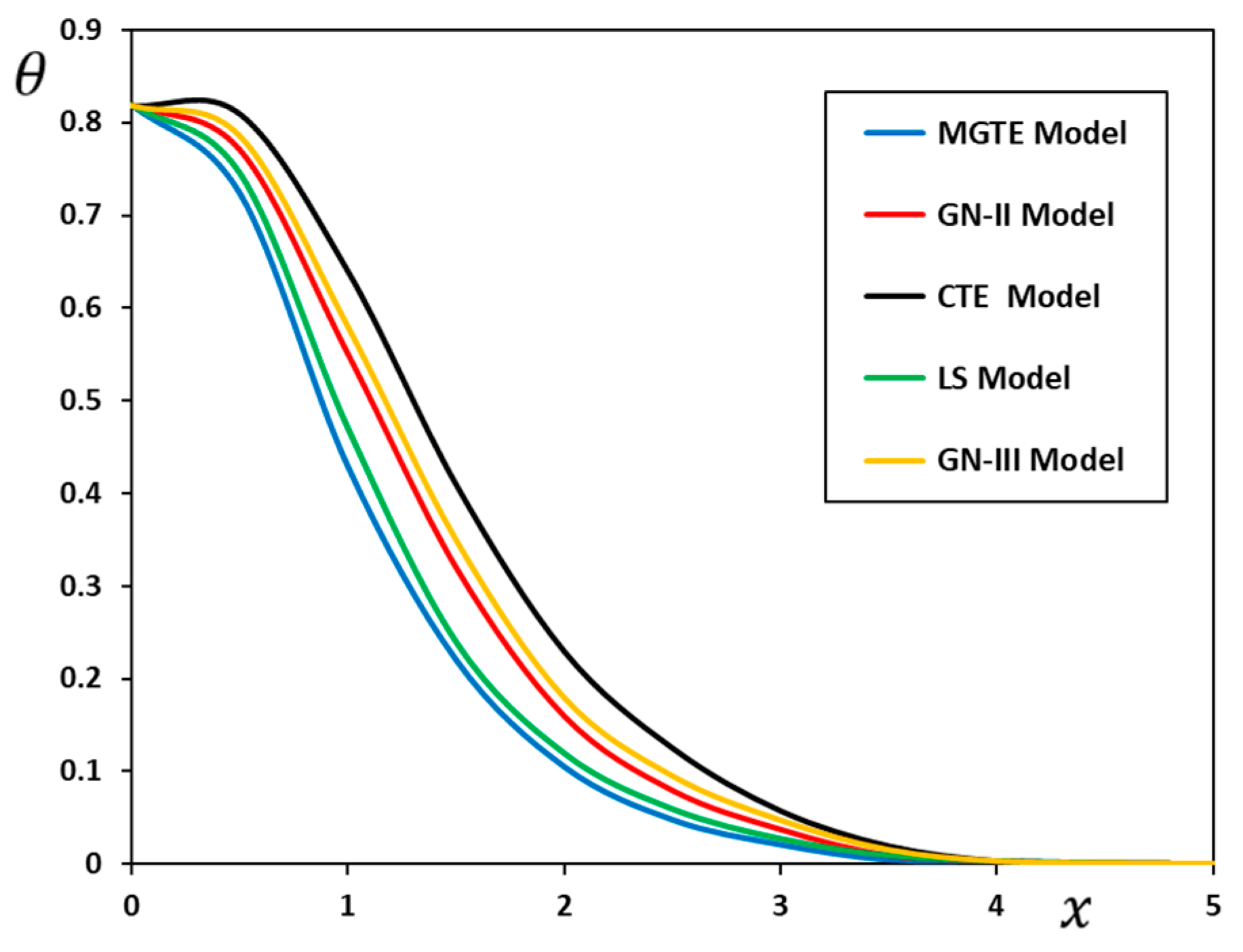
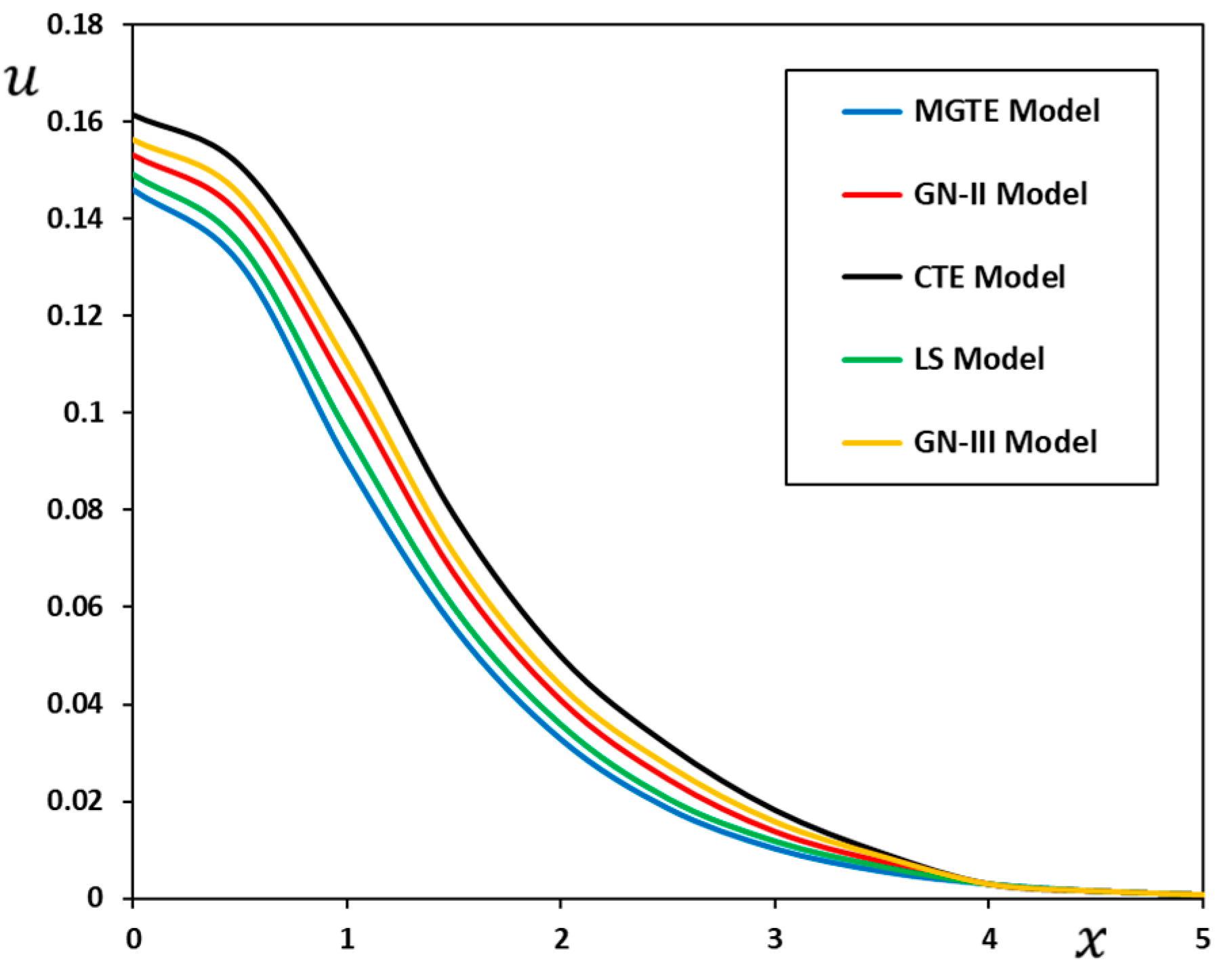
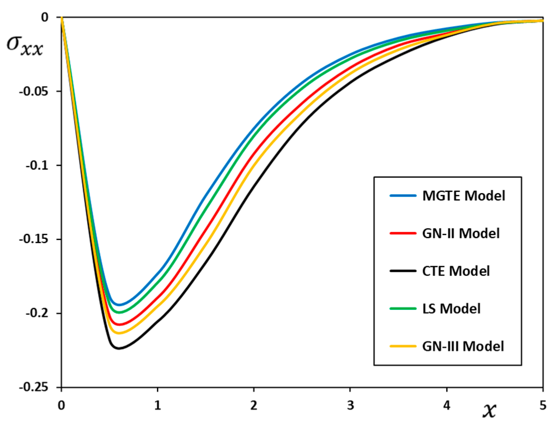
7.1. Comparison of Thermoelastic Models
To avoid the physically impossible contradiction of thermal signals at infinite velocities in linked thermoelasticity, the present model of generalized thermoelasticity is constructed. This subsection of the discussion is devoted to the study of the distributions of different physical fields for different models of thermal elasticity, both conventional and generalized, which can be obtained as special cases of the current Moore–Gibson–Thompson thermoelastic model (MGTE). It can be seen that at
, the coupled thermoelasticity (CTE) model can be derived, while at
, the Lord–Shulman (LS) model can be derived from the proposed model. Also, when
, a system of equations for the Green and Naghdi model (GN-II) can be obtained. Finally, equations of the Green and Naghdi model (GN-III) can be obtained from the present model when the relaxation time parameter is neglected (
). The numerical results of the quantities of the studied fields are represented in
Figure 2,
Figure 3,
Figure 4,
Figure 5,
Figure 6 and
Figure 7 when the non-dimensional values
,
,
, and
are taken into account.
Figure 2.
The temperature change versus for various thermoelastic models when , , and .
Figure 2.
The temperature change versus for various thermoelastic models when , , and .
Figure 3.
The displacement component versus for various thermoelastic models when , , and .
Figure 3.
The displacement component versus for various thermoelastic models when , , and .
Figure 4.
The stress component versus for various thermoelastic models when , , and .
Figure 4.
The stress component versus for various thermoelastic models when , , and .
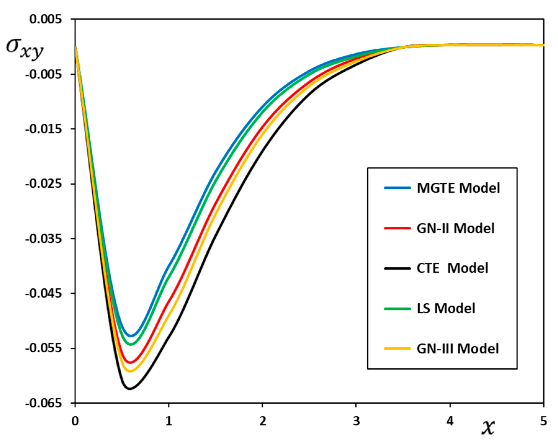
Figure 5.
The stress component versus for various thermoelastic models when , , and .
Figure 5.
The stress component versus for various thermoelastic models when , , and .
Figure 6.
The induced magnetic field versus for various thermoelastic models when , , and .
Figure 6.
The induced magnetic field versus for various thermoelastic models when , , and .
Figure 7.
The induced electric component versus for various thermoelastic models when , , and .
Figure 7.
The induced electric component versus for various thermoelastic models when , , and .
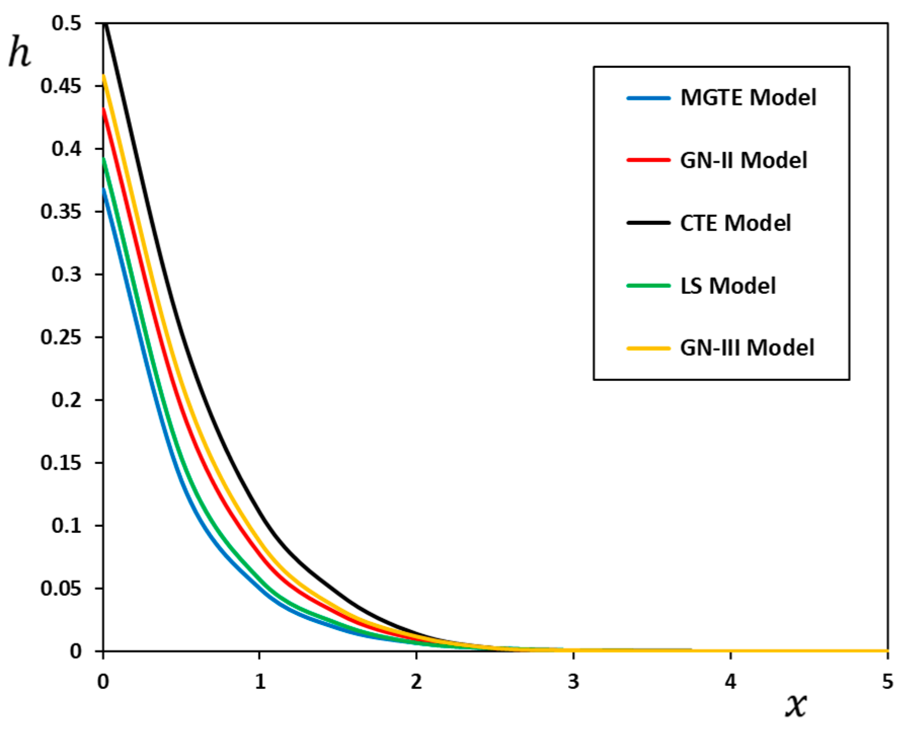
In
Figure 2, the curves depicting the numerical results for the thermal field show that the temperature distribution is prominently near the surface of the half-space due to the presence of the heat source. Moving away from the source, it is seen that the amount of heat decreases with an increasing distance,
, inside the medium.
Figure 3 and
Figure 6 show the change in the displacement component,
and the induced magnetic field,
with changing distance,
, and in the case of several different thermoelastic models. It can be seen from the two figures that the behavior of each of the displacement,
and the induced magnetic field,
, is somewhat similar to the behavior of the thermal field, with different magnitudes and starting points. In
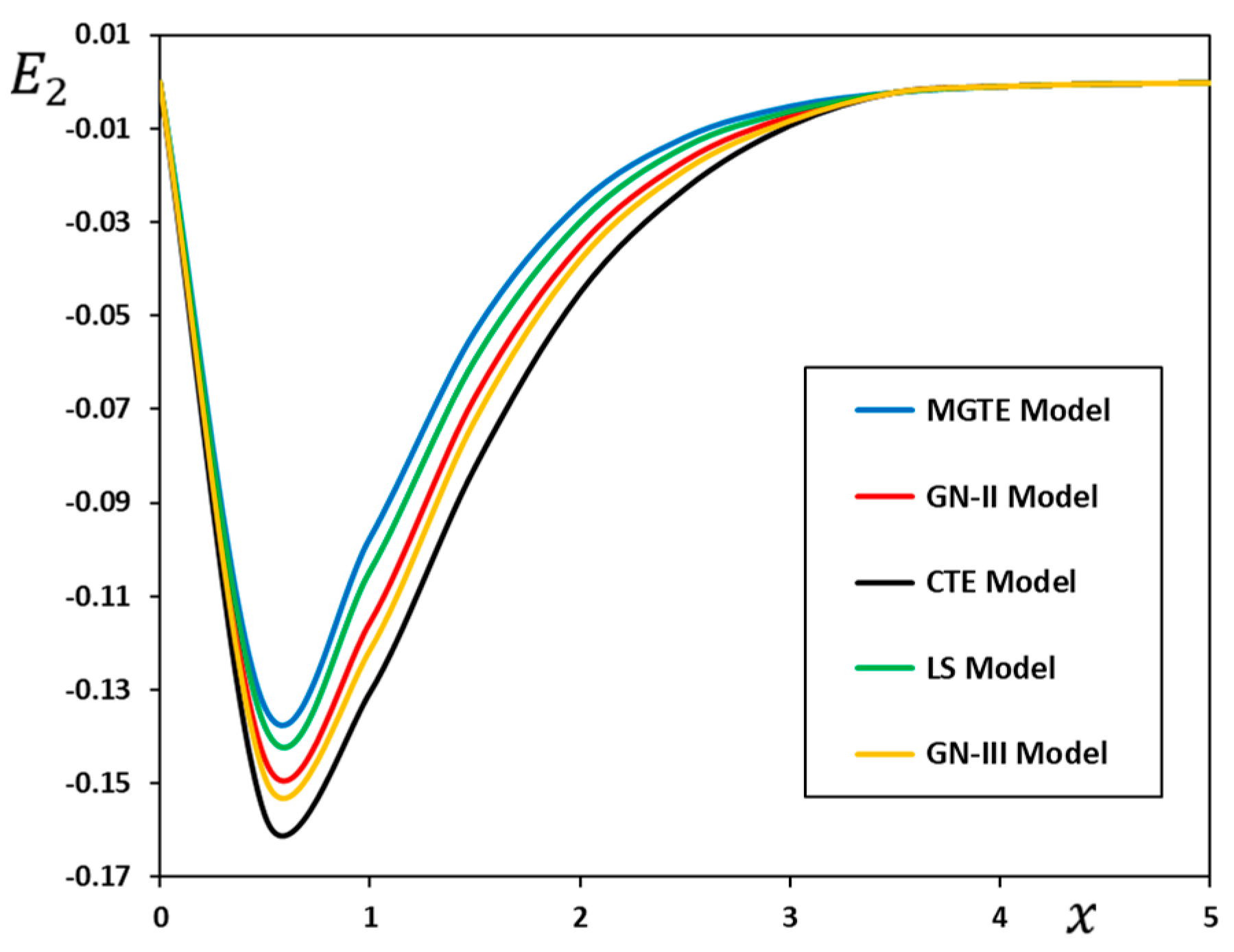
Figure 4,
Figure 5, and
Figure 7, comparisons were made between different thermoelasticity models for each of the thermal stresses (
and
) and the induced electric field component (
). It is noted from these figures that these three domains fulfil the boundary conditions imposed on the problem, as these domains vanish from the free surface of the mediator. Not only that, but it also has the same compressed behavior with different amounts.
The most important results from the numerical results and the different figures can be summarized as follows:
It has been shown that the behavior of the field quantum distributions is quite sensitive to changing the values of the thermodynamic parameters, and
Compared to other extended theories (MGT, LS, GN-II, and GN-III), the coupled theory curves (CTE) are found to be higher than their counterparts are.
Although Biot’s theory (CTE) was applied to many thermoelasticity problems, it produces unacceptable results in situations involving short-range temperatures, such as thermal shocks and laser material interactions.
Extended models contradict the coupled theory, which suggests that heat waves may move at an infinite speed.
The results converged for the two modified generalized theories LS and MGTE. According to the two overarching ideas, a thermoelastic reaction has a “cool-down” period. When the two generalized theories were modified, heat diffusion assumed the appearance of a wave phenomenon rather than the diffusion phenomenon usually associated with the second acoustic effect. The propagation velocity of the heat wave is found to be constrained after modifying the Fourier formula for thermal conductivity in the two theories.
The results demonstrate that the behavior of the various distributions is more pronounced in the case of thermoelastic theory, GN-III, than it is in the case of thermoelastic type, GN-II. One possible explanation is that there is no energy loss in the second form.
The numerical findings distinguish between the Green and Naghdi GN-III theories and the novel MGTE model, as well as other generalized thermal models. The GN-III model relies more on the classic theory of thermoelasticity and shows a greater temperature change than the MGTE model does. This result confirms the validity of the current model, which suggests that the GN-III model follows the behavior of the traditional theory that predicts infinite velocities for heat waves.
Since the relaxation time, is factored into the heat equation, the solutions converge in both the MGTE and LS models. This means that the presence of relaxation time leads to a reduction in the propagation of thermal and mechanical waves in accordance with the experimental results.
In reality, the strain and stress fields are affected by the fluctuating core body temperature, and the reverse is also true. Force loads, as well as temperature stresses, are common conditions for many structural parts. The material might crack under these forces or under the combined mechanical and thermal stresses resulting from external loads. The amount and distribution of thermal stresses must be determined for a comprehensive strength study of structures. Because of this, professionals from a wide range of areas focus their attention on problems related to calculating temperature fields and thermal stresses.
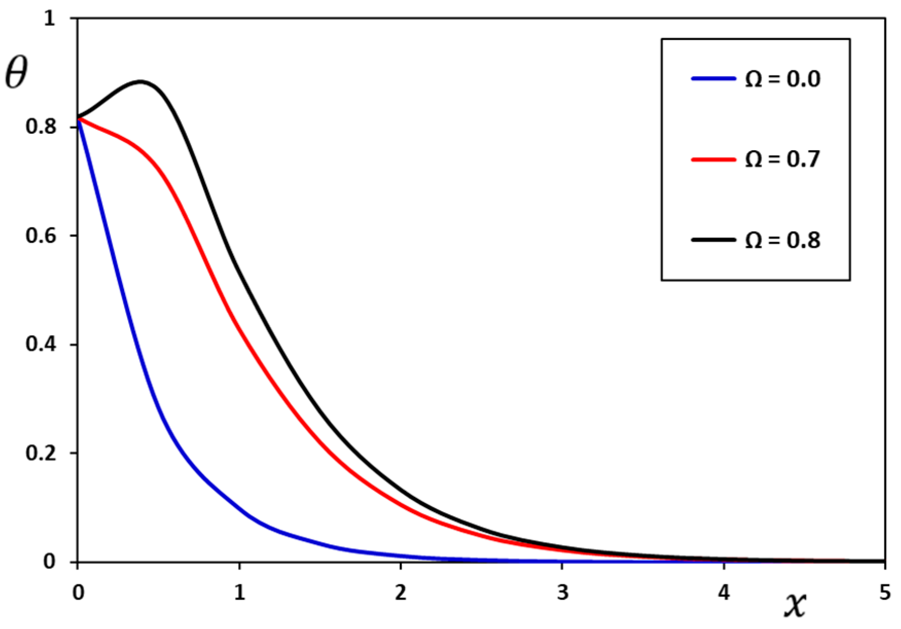
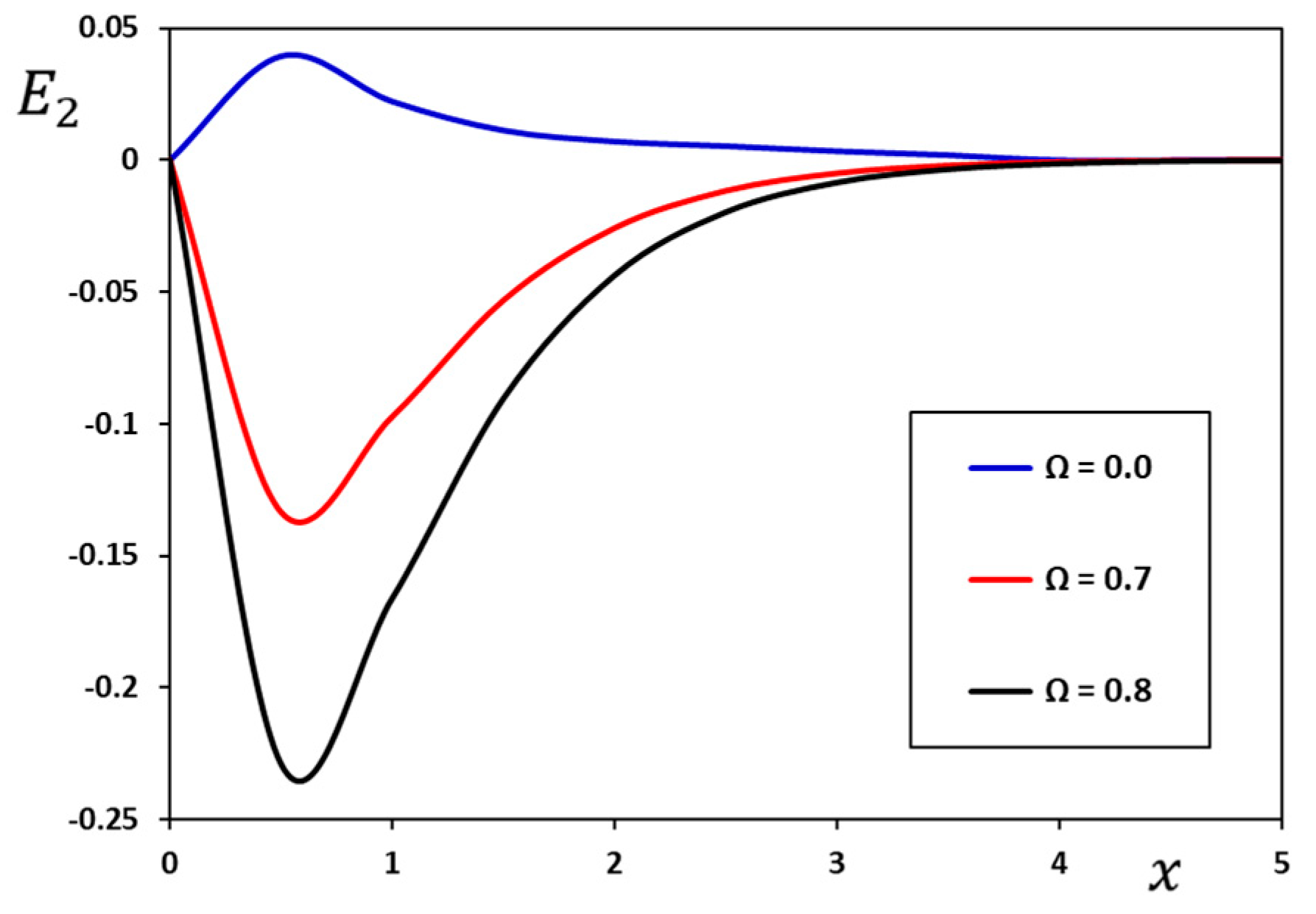
7.2. Effect of the Angular Velocity on Variables of the Problem
A lot of research has been conducted on the topic of the propagation of elastic waves in rotating bodies. However, the amount of research on rotating thermoelastic materials within a magnetic field is minimal. If the coordinate system is assumed to be fixed in a rotating medium, then the equations of motion must include the effects of Coriolis gravity and acceleration. As a result of including centripetal and Coriolis accelerations into the equations of motion with regard to a rotating frame of reference, the medium takes on the properties of a dispersive and anisotropic medium.
This theoretical paper considers wave propagation in a linear, homogeneous, isotropic thermoelastic medium, where the entire elastic material is assumed to rotate at the same angular velocity,
. This subsection investigates how the behavior of the investigated physical fields changes as the value of the regulated angular velocity,
changes. The numerical values of non-dimensional fields over a wide range of
are computed when the values
,
and
are taken. Also, the Moore–Gibson–Thompson extended thermoelastic is will only be taken into account when the three curves shown in
Figure 8,
Figure 9,
Figure 10,
Figure 11,
Figure 12 and
Figure 13 are plotted. Three different values of the angular velocity of rotation
,
and
are taken into account. It is noted that when there is no effect of rotation,
is set. The rotation of astronomical entities and the moon are examples of the numerous real-world challenges that benefit from understanding how plane waves propagate in a rotating medium.
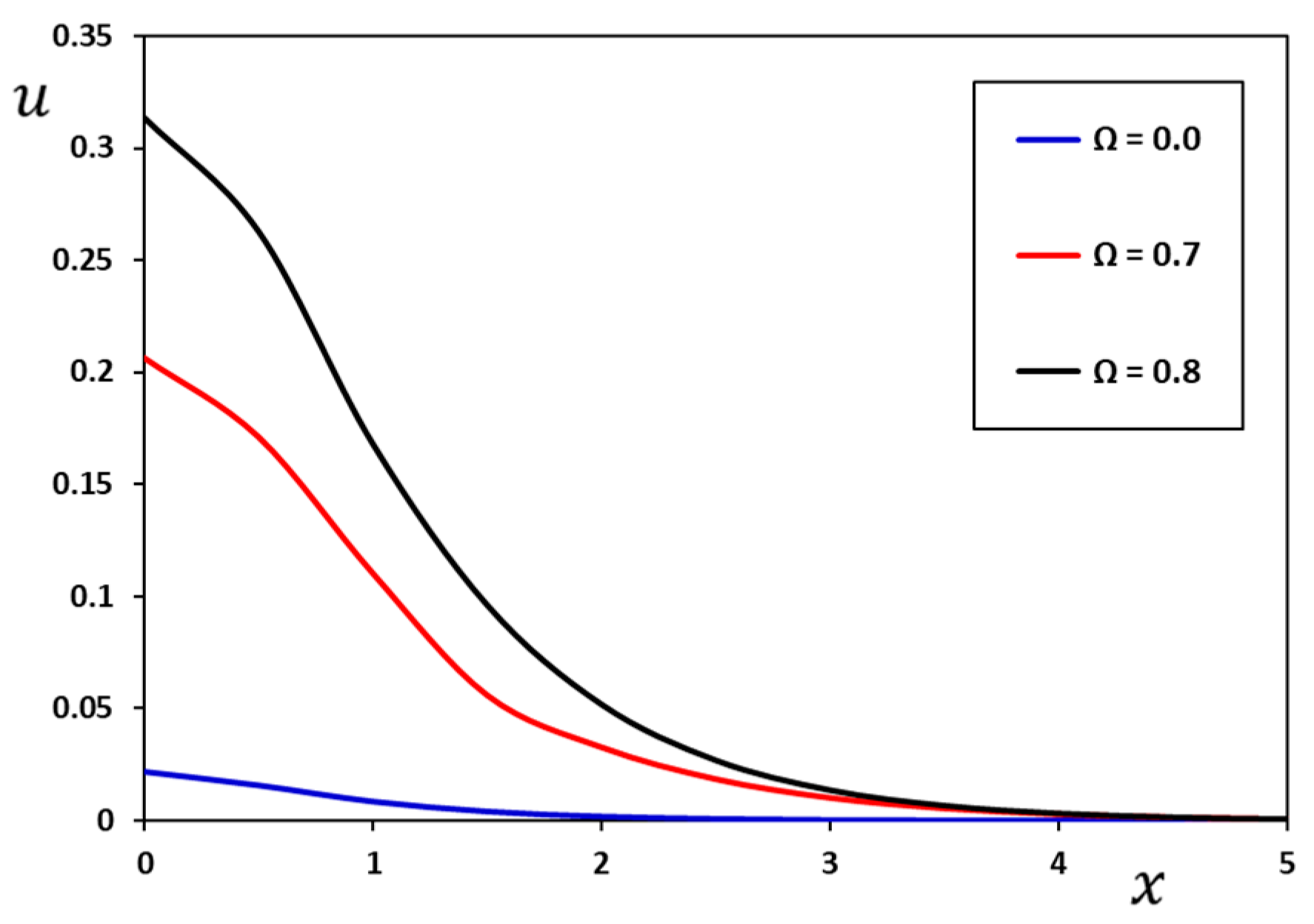
Figure 8.
Impact of rotational speed, on the temperature change, .
Figure 8.
Impact of rotational speed, on the temperature change, .
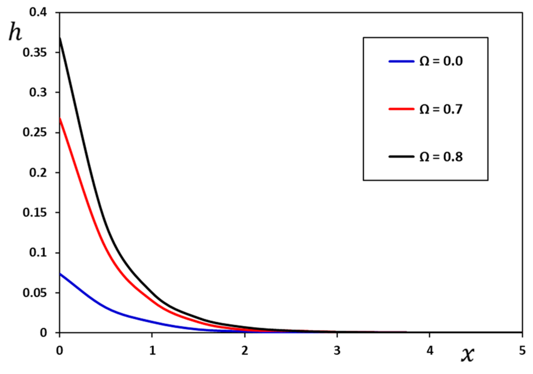
Figure 9.
Impact of rotational speed, on the displacement component, when , , and .
Figure 9.
Impact of rotational speed, on the displacement component, when , , and .
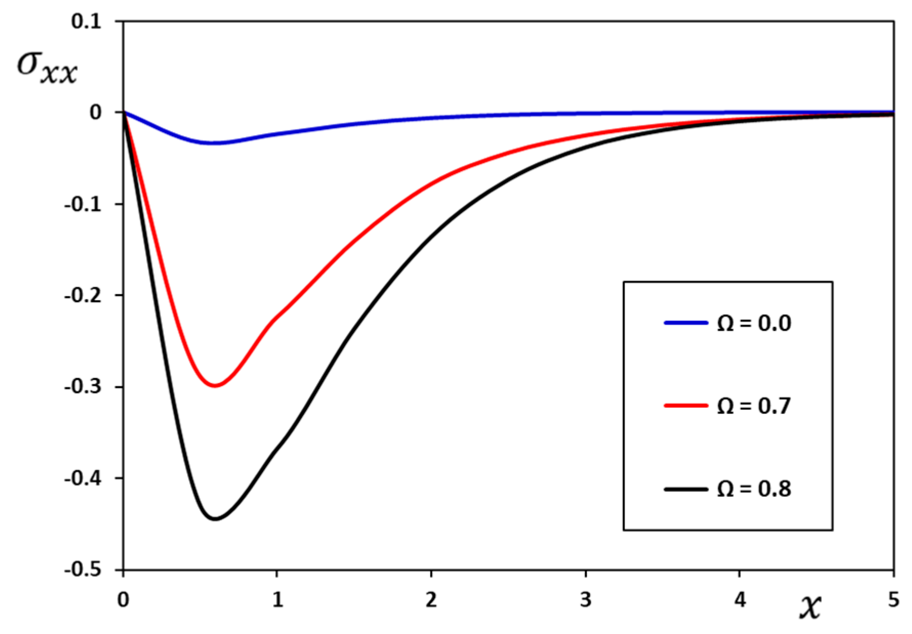
Figure 10.
Impact of rotational speed, on the stress component, when , , and .
Figure 10.
Impact of rotational speed, on the stress component, when , , and .
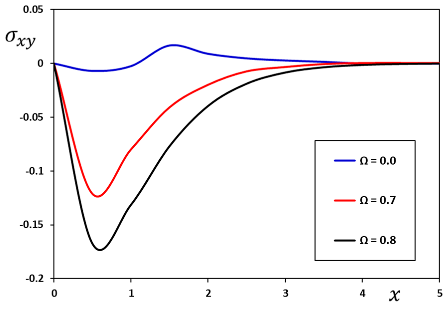
Figure 11.
Impact of rotational speed, on the stress component, when , , and .
Figure 11.
Impact of rotational speed, on the stress component, when , , and .
Figure 12.
Impact of rotational speed, on the induced magnetic field, , when , , and .
Figure 12.
Impact of rotational speed, on the induced magnetic field, , when , , and .
Figure 13.
Impact of rotational speed, on the induced electric component, when , , and .
Figure 13.
Impact of rotational speed, on the induced electric component, when , , and .
From the figures, the most important conclusions can be summarized as follows:
It has been shown that rotation has a significant effect on the variance of all physical fields considered in the studied problem.
The initial value of some system variables is the same and may be zero according to the boundary criteria.
The insights from the current theoretical conclusions may be useful to experimental investigators, engineers, and seismologists who study the field of spinning bodies.
Temperature, travels through the medium in a wave pattern at finite speeds. With increasing values of the angular velocity of rotation, , the temperature distributions increase.
There is a significant difference in deformation in the presence and absence of rotation. Both the deformation and the magnetic induction field increase significantly with the increase in the constant angular velocity of rotation, .
The change in the angular velocity of the body’s rotation has a significant impact on the thermal stresses inside the medium. The amount of compressive behavior of the stresses increases with the increase in the amount of rotation.
The proposed results may have significant technological applications, including designing and constructing gyroscopes and other rotating sensors, because the rotational change affects different domains in various ways.
Investigating issues of thermoelasticity in rotating media makes more sense because of the angular velocity of small objects that go into designing machines as well as massive bodies such as the Earth, Moon, and other planets.
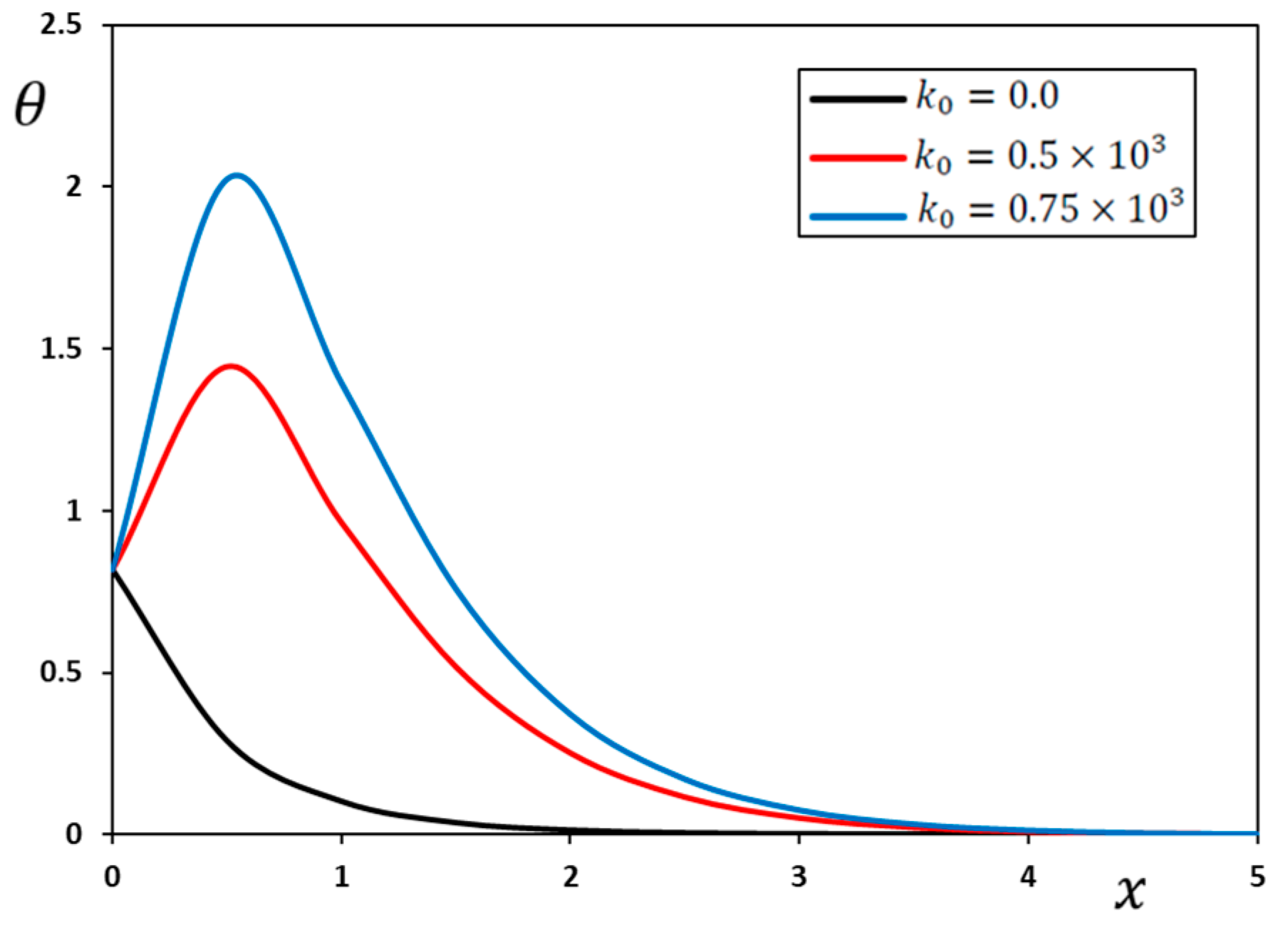
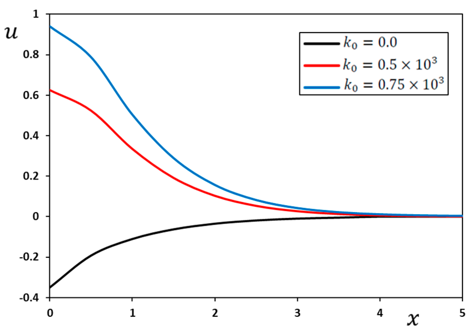
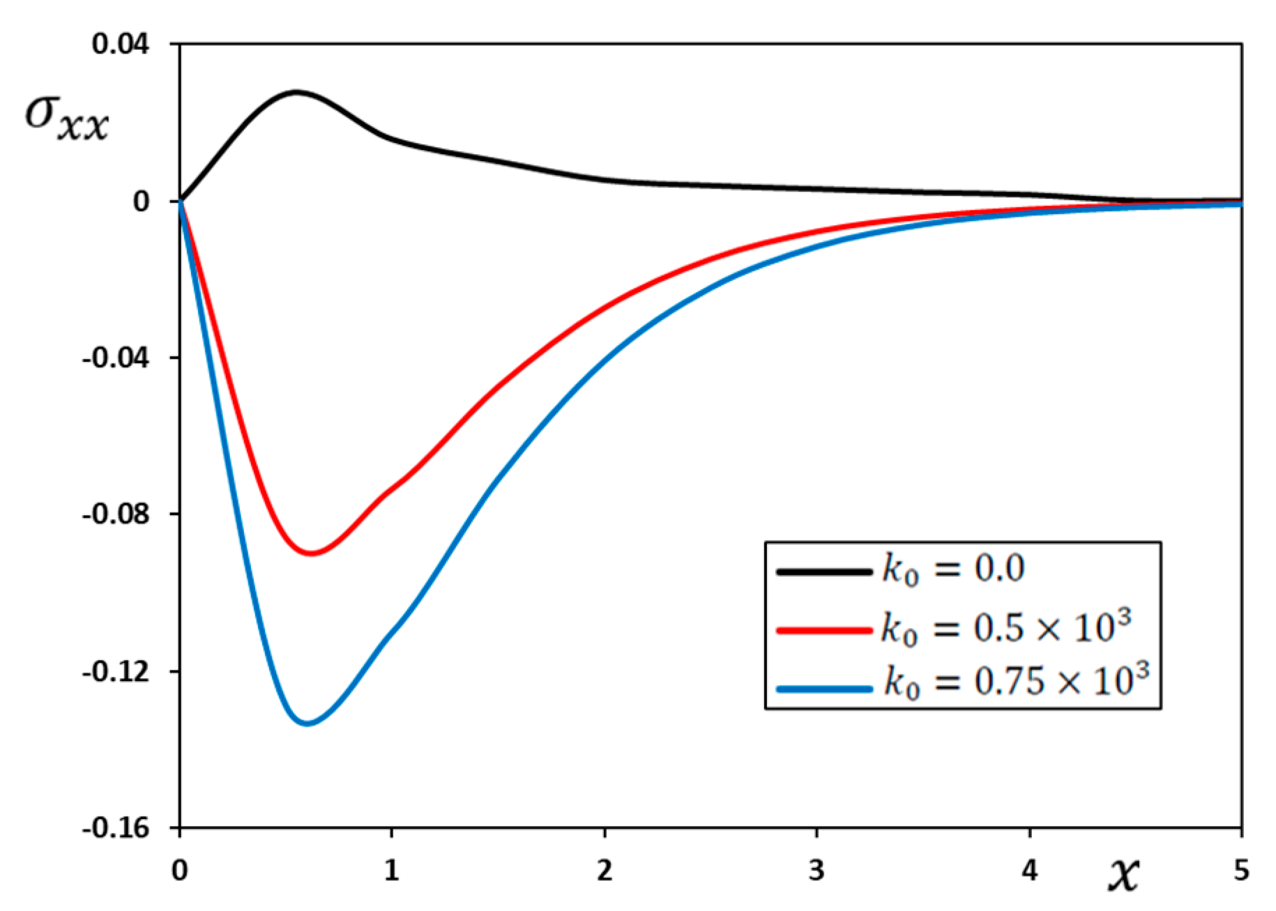
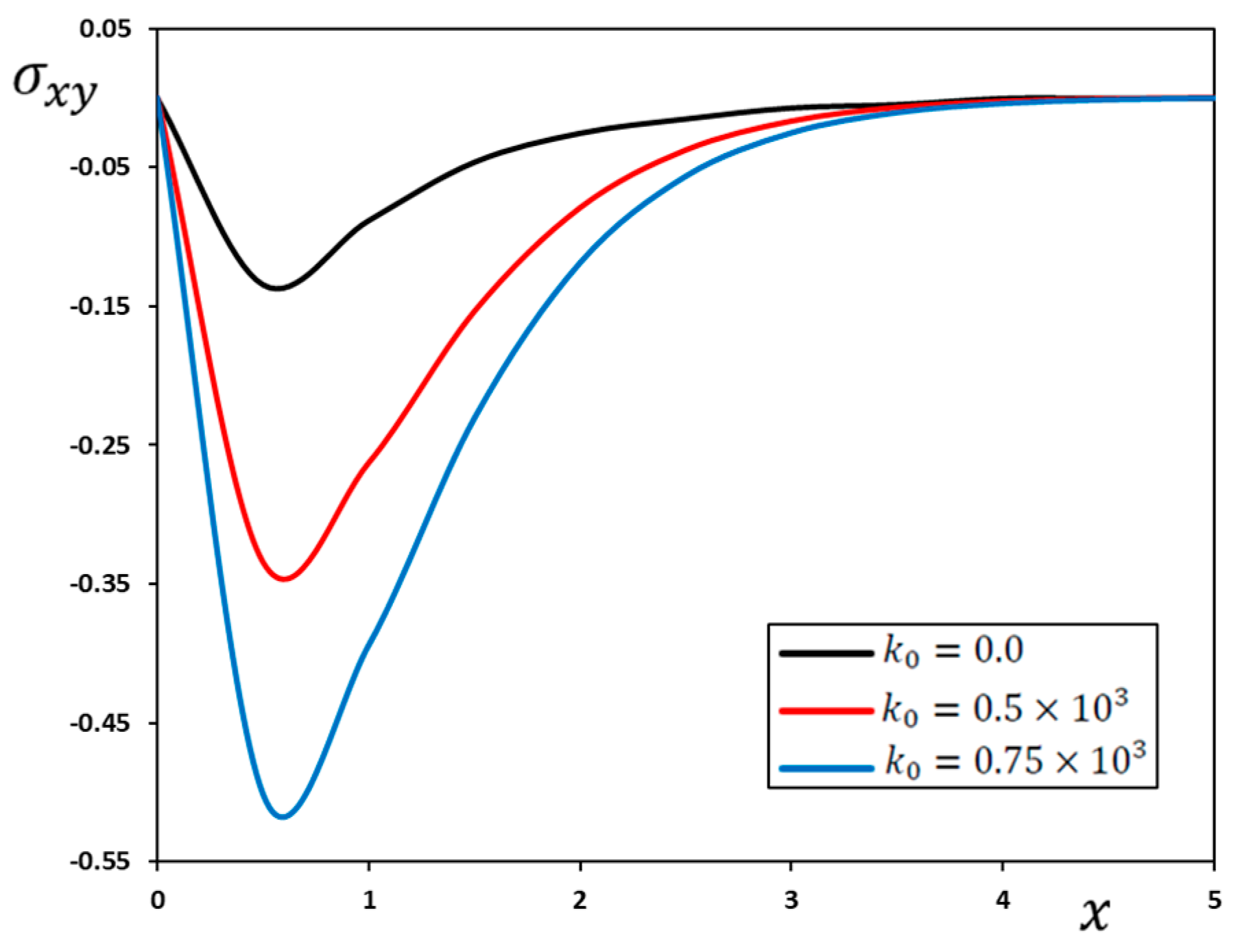
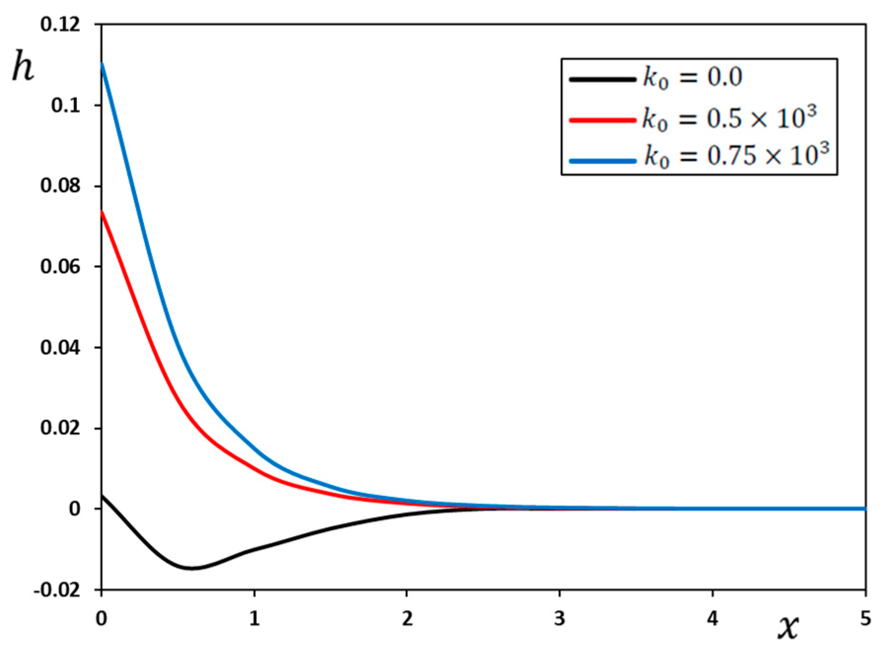
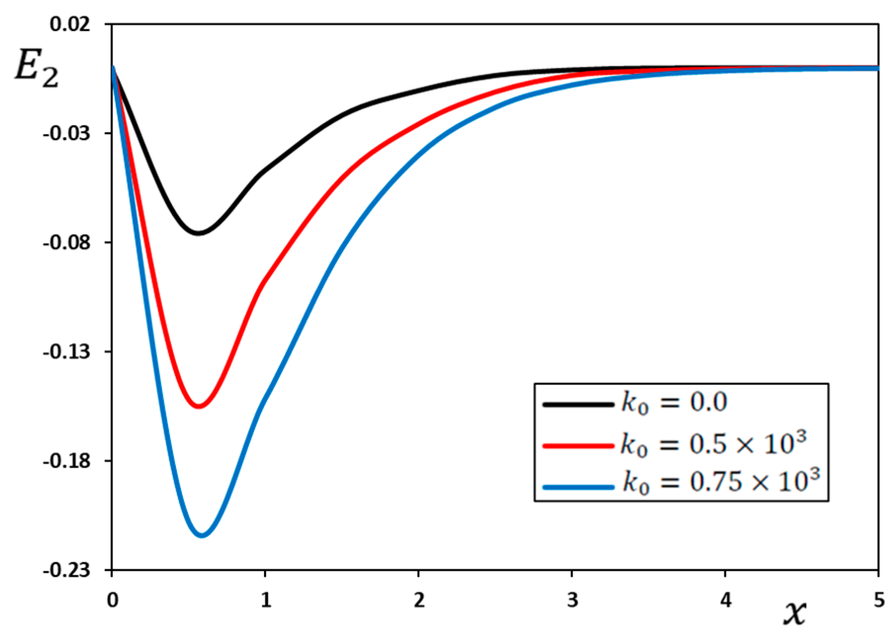
7.3. Effect of the Modified Ohm’s Law Coefficient on Variables of the Problem
Wave propagation in isotropic thermoelastic media has been extensively studied in the literature in the presence of an acting magnetic field. Their potential use in the non-destructive testing of composite structures used in aerospace, automobiles, and other technical fields makes them interesting. Researchers have been looking at the electromagnetic response in the thermomechanical behaviors of materials since the 18th century when the concept of energy conversion was first introduced. Thermoelastic electromagnetic materials have been shown to be naturally isotropic and couple with electric, magnetic, and mechanical fields. In addition, these electromagnetic materials have many practical uses, including in lasers, supersonic devices, microwave ovens, and even smart applications. The current paper focuses on studies of the effect of a magnetic field on a thermoelastic medium based on the MGTE model of thermoelasticity. These types of problems in the magnetic field are essential to many dynamical systems. Because it has such wide-ranging implications, studies examining how the fundamental magnetic field affects thermoelasticity theory have attracted the attention of many experts.
Ohm’s law has been changed by taking into account the effect of the temperature gradient. The current strength at each site is inversely proportional to the voltage gradient. In this sub-case of research, the effect of changing the Ohm’s law modulation coefficient,
on the behavior of various fields is being investigated. The results of calculations for the real part of various non-dimensional domains are represented in
Figure 14,
Figure 15,
Figure 16,
Figure 17,
Figure 18 and
Figure 19 at the plane,
. It was also taken into account that the study was carried out in the case of the modified Moore–Gibson–Thompson (MGTE) model of thermoelasticity with a single relaxation period when
and
.
When the time, and the initial magnetic field, are constant, how the non-dimensional temperature, displacement components, thermal stresses, and induced magnetic and electric fields with different values of Ohm’s law coefficient () change in the direction of the depth of the medium are studied. For two separate scenarios, numerical computations are made: , and . The different figures indicate the coupled effects of electromagnetism and thermoelasticity on physical quantities.
Figure 14.
Influence of the coefficient, on the temperature change, when , , and .
Figure 14.
Influence of the coefficient, on the temperature change, when , , and .
Figure 15.
Influence of the coefficient, the displacement component, when , , and .
Figure 15.
Influence of the coefficient, the displacement component, when , , and .
Figure 16.
Influence of the coefficient, on the stress component, when , , and .
Figure 16.
Influence of the coefficient, on the stress component, when , , and .
Figure 17.
Influence of the coefficient, on the stress component, when , , and .
Figure 17.
Influence of the coefficient, on the stress component, when , , and .
Figure 18.
Influence of the coefficient, on the induced magnetic field, when , , and .
Figure 18.
Influence of the coefficient, on the induced magnetic field, when , , and .
Figure 19.
Influence of the coefficient, on the induced electric component, when , , and .
Figure 19.
Influence of the coefficient, on the induced electric component, when , , and .
The following most important conclusions can also be summarized:
To a large extent, the electromagnetic field affects the distributions of all studied physical quantities, both with and without the electromagnetic field.
Due to the influence of the magnetic field, the values of all physical variables become zero as x increases, and all the functions examined have continuous curves.
When the temperature gradient coefficient, is increased, the modified Ohm’s law leads to an increase in temperature change, . It is noted that the thermal diffusion is much greater than it is in the case of neglecting this factor, . For this reason, this effect must be taken into account in the design of some thermoelectric devices.
It is seen that the Seebeck modulus has a prominent effect on deformation. One of the observations that must be taken into account is that deformation behavior in the case of neglecting this parameter is the opposite of the behavior in the case of taking it into account.
The Seebeck coefficient has a compressive effect on the behavior of thermal stresses and the induced electric field component. The higher the value of the temperature gradient coefficient in the modified Ohm’s law is, the greater the magnitudes of these quantities are.
One of the many crucial elements in the effective operation of thermoelectric generators and thermoelectric coolers is the use of materials with a high Ohm’s law coefficient (Seebeck coefficient).
8. Conclusions
In this investigation, we considered how thermomechanical waves’ behavior is affected in thermoelastic, isotropic, and fully conductive materials due to the propagation of elastic thermo-electromagnetic waves on their surface. For this purpose, the Moore–Gibson–Thompson thermoelasticity model was considered in addition to the modified Ohm’s law.
From the discussion of the numerical results, it was found that the coupling behaviors of thermoelastic electromagnetic materials and electric, magnetic, and mechanical fields are correlated. The results obtained can, therefore, be used in various applications, including computers, microwave ovens, lasers, and other electromagnetic devices. It is also shown by the experimental results that when thermal shock is applied, the thermal disturbance appears quickly, and then dissipates far from the disturbance area. Also, the amount of thermal deformation in the case of the GN-III model is greater than that in the case of the MGT model, which means that it does not fade quickly inside the medium. This result proves the importance of the model proposed in this article. Since the relaxation time, is factored into the heat equation, the solutions converge in both the MGTE and LS models. This means that the presence of relaxation time leads to a reduction in the propagation of thermal and mechanical waves, which is in accordance with the experimental results.
There is a significant difference in deformation in the presence and absence of rotation. Both the deformation and the magnetic induction fields increase significantly with the increase in the constant angular velocity of rotation. The change in the angular velocity of the body’s rotation has a significant impact on the thermal stresses inside the medium. The amount of compressive behavior of the stresses increases with the increase in the amount of rotation. The proposed results may have significant technological applications, including designing and constructing gyroscopes and other rotating sensors, because rotational change affects different domains in various ways.
Also, it was found that the coupling behaviors of thermoelastic electromagnetic materials and electric, magnetic, and mechanical fields are correlated. The Seebeck coefficient has a compressive effect on the behavior of thermal stresses and the induced electric field component. One of the crucial elements in the effective operation of thermoelectric generators and thermoelectric coolers is using materials with a high Ohm’s law coefficient (Seebeck coefficient).
The results obtained can, therefore, be used in various applications, including computers, microwave ovens, lasers, and other electromagnetic devices. It is also shown by the experimental results that when thermal shock is applied, the thermal disturbance appears quickly, and then dissipates far from the disturbance area. In the future, the results presented in this paper can be generalised to include smart materials science and the design of new heterogeneous materials and small, nanoscale devices.


