
An Exponentiated Skew-Elliptic Nonlinear Extension to the Log–Linear Birnbaum–Saunders Model with Diagnostic and Residual Analysis

Abstract
:1. Introduction
2. New Model
Nonlinear Log–BS Model
- The pdf and cdf:which we denote by and
- Percentiles:If , following the uniform distribution, then the random variableis distributed according to the SEXPsn distribution, with parameters , 2, and , where is the inverse of the skew-normal distribution.
- Flexibility:
- (a)
- follows the power-normal (exponentiated-normal) nonlinear regression model.
- (b)
- follows the skew-normal nonlinear regression model.
- (c)
- and follow the normal nonlinear regression model.
Hence, in terms of skewness and kurtosis, this model is more flexible than the power-normal, skew-normal, and normal nonlinear models. - Let . Then, for constants and
- If , then
- Let . Then,
- Expectation and variance:whereandwith representing the variance of the random variable where
3. Diagnostic Analysis
3.1. Local Influence
- The normal curvature, conforming in any direction to , is invariant under reparametrization.
- In any direction therefore, is a normalized measure, which will allow comparisons of the curvatures.
3.2. Local Influence for the Nonlinear Log–BS Exponentiated Skew-Normal Model
3.2.1. Weighting Cases
3.2.2. Perturbation in the Response Variable
3.2.3. Perturbation in the Explanatory Variable
3.3. Residual Analysis
3.3.1. Residual Components
3.3.2. Standardized Residuals
4. Simulation Study
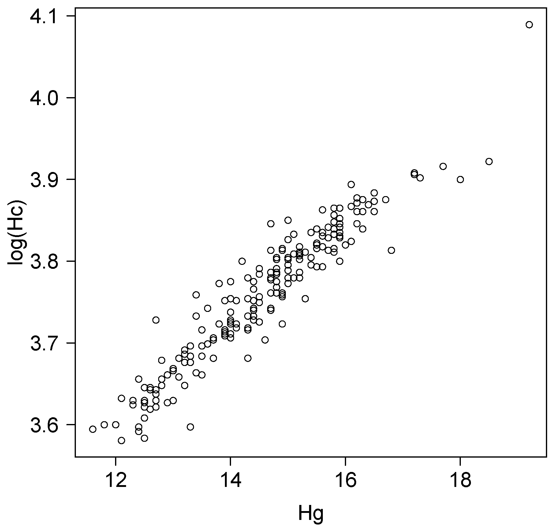
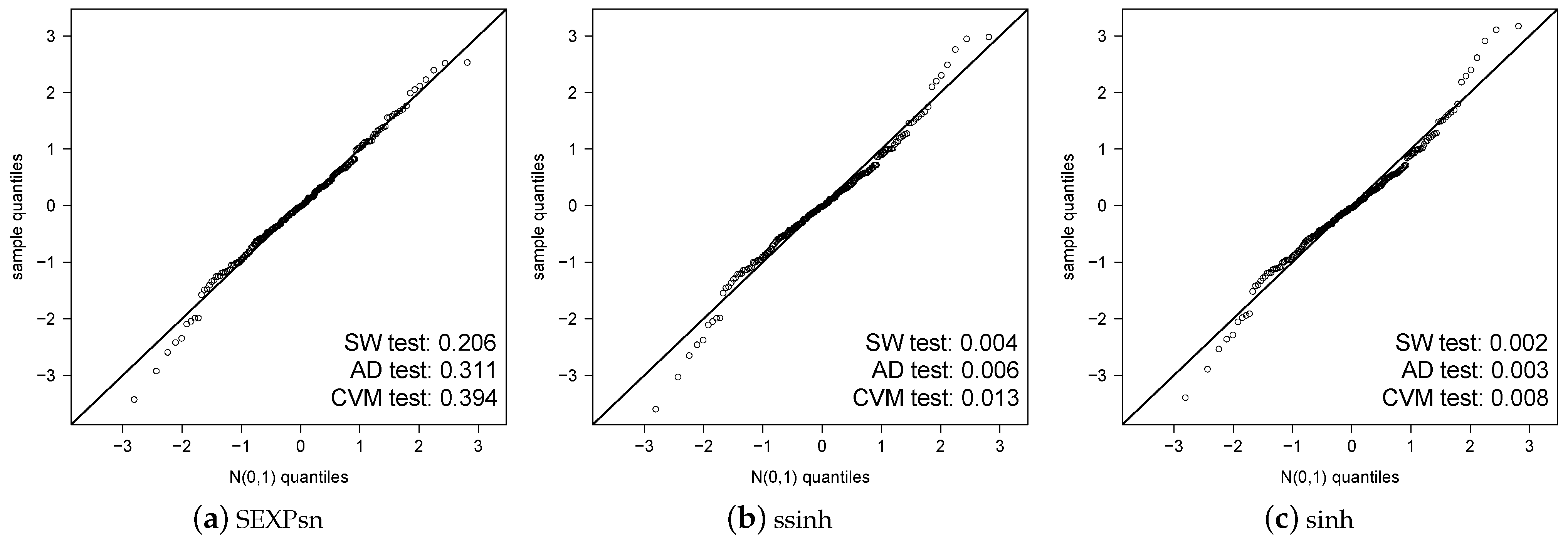
5. Application
- A linear relation: ; and
- A nonlinear relation: .
6. Conclusions
Author Contributions
Funding
Institutional Review Board Statement
Informed Consent Statement
Data Availability Statement
Acknowledgments
Conflicts of Interest
Appendix A. The Elements of the Information Matrix
Appendix B. Definitions of κji for j = 1, 2, …, 8
References
- Cancho, V.G.; Lachos, V.H.; Ortega, E.M.M. A nonlinear regression model with skew-normal errors. Stat. Pap. 2010, 51, 547–558. [Google Scholar] [CrossRef]
- Martínez-Flórez, G.; Bolfarine, H.; Gómez, H.W. Likelihood-based inference for the power regression model. SORT-Stat. Oper. Res. Trans. 2015, 39, 187–208. [Google Scholar]
- Lemonte, A.J.; Cordeiro, G.M. Birnbaum–Saunders nonlinear regression models. Comput. Stat. Data Anal. 2010, 53, 4441–4452. [Google Scholar] [CrossRef] [Green Version]
- Lemonte, A. A log-Birnbaum-Saunders Regression Model with Asymmetric Errors. J. Stat. Comput. Simul. 2012, 82, 1775–1787. [Google Scholar] [CrossRef] [Green Version]
- Martínez-Flórez, G.; Bolfarine, H.; Gómez, H.W. An extension of the generalized Birnbaun-Saunders distribution. Stat. Probab. Lett. 2017, 19, 913–933. [Google Scholar]
- Cambanis, S.; Huang, S.; Simons, G. On the Theory of Elliptically Contoured Distributions. J. Multivar. Anal. 1981, 11, 365–385. [Google Scholar] [CrossRef] [Green Version]
- Fang, K.T.; Kotz, S.; Ng, K.W. Symmetric Multivariate and Related Distribution; Chapman and Hall: London, UK, 1990. [Google Scholar]
- Gupta, A.K.; Varga, T. Elliptically Contoured Models in Statistics; Kluwer Academic Publishers: Boston, MA, USA, 1993. [Google Scholar]
- Díaz-García, J.A.; Leiva-Sánchez, V. A new family of life distributions based on the elliptically contoured distributions. J. Statist. Plann. Inference 2005, 128, 445–457. [Google Scholar] [CrossRef]
- Kelker, D. Distribution Theory of Spherical Distributions and a Location Scale Parameter Generalization. Sankhya Ser. A 1970, 32, 419–430. [Google Scholar]
- Lachos, V.H.; Bolfarine, H.; Arellano-Valle, R.B.; Montenegro, L.C. Likelihood-based inference for multivariate skew-normal regression models. Commun. Stat. Theory Methods 2007, 36, 1769–1786. [Google Scholar] [CrossRef]
- Azzalini, A. A class of distributions which includes the normal ones. Scand. J. Stat. 1985, 12, 171–178. [Google Scholar]
- Owen, D.B. Tables for computing bi-variate normal probabilities. Ann. Math. Stat. 1956, 27, 1075–1090. [Google Scholar] [CrossRef]
- Durrans, S.R. Distributions of fractional order statistics in hydrology. Water Resour. Res. 1992, 28, 1649–1655. [Google Scholar] [CrossRef]
- Pewsey, A.; Gómez, H.; Bolfarine, H. Likelihood-based inference for power distributions. Test 2012, 21, 775–789. [Google Scholar] [CrossRef]
- Birnbaum, Z.W.; Saunders, S.C. A New Family of Life Distributions. J. Appl. Probab. 1969, 6, 319–327. [Google Scholar] [CrossRef]
- Castillo, N.O.; Gómez, H.W.; Bolfarine, H. Epsilon Birnbaum–Saunders distribution family: Properties and inference. Stat. Pap. 2011, 6, 871–883. [Google Scholar] [CrossRef]
- Gómez, H.W.; Olivares-Pacheco, J.F.; Bolfarine, H. An extension of the generalized Birnbaun-Saunders distribution. Stat. Probab. Lett. 2009, 79, 331–338. [Google Scholar] [CrossRef]
- Rieck, J.R.; Nedelman, J.R. A log-linear model for the Birnbaum-Saunders distribution. Technometrics 1991, 33, 51–60. [Google Scholar]
- Barros, M.; Paula, G.A.; Leiva, V. A new class of survival regression models with heavy-tailed errors: Robustness and diagnostics. Lifetime Data Anal. 2008, 14, 316–332. [Google Scholar] [CrossRef]
- Leiva, V.; Vilca, F.; Balakrishnan, N.; Sanhueza, A. A skewed sinh-normal distribution and its properties and application to air pollution. Commun. Stat. Theory Methods 2010, 39, 426–443. [Google Scholar] [CrossRef]
- Santana, L.; Vilca, F.; Leiva, V. Influence analysis in skew-Birnbaum-Saunders regression models and applications. J. Appl. Stat. 2011, 38, 1633–1649. [Google Scholar] [CrossRef]
- Martínez-Flórez, G.; Bolfarine, H.; Gómez, H.W. Skew-normal alpha power model. Statistics 2014, 48, 1414–1428. [Google Scholar] [CrossRef]
- Martínez-Flórez, G.; Bolfarine, H.; Gómez, Y.M. The Skewed-Elliptical Log–Linear Birnbaum–Saunders Alpha-Power Model. Symmetry 2021, 13, 1297. [Google Scholar] [CrossRef]
- Cook, R.D. Assessment of local influence. J. R. Stat. Soc. B 1986, 48, 133–169. [Google Scholar] [CrossRef]
- Galea, M.; Leiva, V.; Paula, G.A. Influence diagnostics in log-Birnbaum-Saunders regression models. J. Appl. Stat. 2004, 31, 1049–1064. [Google Scholar] [CrossRef]
- Lesaffre, E.; Verbeke, G. Local influence in linear mixed models. Biometrics 1998, 54, 570–582. [Google Scholar] [CrossRef] [PubMed]
- Verbeke, G.; Molenberghs, G. Linear Mixed Models for Longitudinal Data; Springer: New York, NY, USA, 2000. [Google Scholar]
- Poon, W.Y.; Poon, Y.S. Conformal normal curvature and assessment of local influence. J. R. Stat. Soc. B 1999, 61, 51–61. [Google Scholar] [CrossRef]
- Wei, B.C.; Hu, Y.Q.; Fung, W.K. Generalized leverage and its applications. Scand. J. Stat. 1998, 25, 25–37. [Google Scholar] [CrossRef]
- Azzalini, A. The R Package ’sn’: The Skew-Normal and Related Distributions such as the Skew-t and the SUN (Version 2.1.0). 2022. Available online: https://cran.r-project.org/package=sn (accessed on 15 October 2022).
- R Core Team. R: A Language and Environment for Statistical Computing; R Foundation for Statistical Computing: Vienna, Austria, 2022; Available online: https://www.R-project.org/ (accessed on 15 October 2022).
- Akaike, H. A new look at statistical model identification. IEEE Trans. Autom. Control 1974, 19, 716–723. [Google Scholar] [CrossRef]


| True Values | |||||||||||||||
|---|---|---|---|---|---|---|---|---|---|---|---|---|---|---|---|
| param. | bias | SE1 | SE2 | CP | bias | SE1 | SE2 | CP | bias | SE1 | SE2 | CP | |||
| 0.5 | −0.168 | 0.372 | 0.269 | 0.940 | −0.094 | 0.275 | 0.205 | 0.940 | −0.038 | 0.066 | 0.055 | 0.949 | |||
| −0.069 | 0.648 | 0.467 | 0.927 | −0.024 | 0.372 | 0.293 | 0.933 | −0.013 | 0.120 | 0.100 | 0.947 | ||||
| 0.036 | 0.116 | 0.088 | 0.921 | 0.009 | 0.071 | 0.053 | 0.933 | 0.006 | 0.017 | 0.015 | 0.947 | ||||
| 0.491 | 0.880 | 0.523 | 0.872 | 0.138 | 0.514 | 0.402 | 0.910 | 0.071 | 0.144 | 0.128 | 0.945 | ||||
| −1.232 | 2.974 | 1.932 | 0.994 | −0.455 | 1.584 | 1.270 | 0.978 | −0.188 | 0.561 | 0.493 | 0.972 | ||||
| −0.532 | 0.847 | 0.518 | 0.877 | −0.155 | 0.454 | 0.348 | 0.891 | −0.073 | 0.127 | 0.110 | 0.950 | ||||
| 0.210 | 2.414 | 1.690 | 0.917 | 0.057 | 1.331 | 1.020 | 0.939 | 0.033 | 0.307 | 0.270 | 0.946 | ||||
| 0.079 | 0.507 | 0.383 | 0.935 | 0.030 | 0.339 | 0.281 | 0.940 | 0.013 | 0.082 | 0.072 | 0.946 | ||||
| −0.037 | 0.171 | 0.120 | 0.902 | −0.011 | 0.114 | 0.086 | 0.931 | −0.004 | 0.037 | 0.032 | 0.948 | ||||
| −0.433 | 0.715 | 0.441 | 0.909 | −0.125 | 0.336 | 0.268 | 0.935 | −0.068 | 0.098 | 0.084 | 0.947 | ||||
| −1.437 | 3.754 | 2.454 | 0.972 | −0.464 | 2.218 | 1.782 | 0.964 | −0.229 | 0.821 | 0.685 | 0.959 | ||||
| 0.816 | 2.157 | 1.347 | 0.894 | 0.269 | 1.241 | 1.006 | 0.909 | 0.113 | 0.438 | 0.395 | 0.947 | ||||
| 1.8 | 0.208 | 3.244 | 2.259 | 0.933 | 0.071 | 2.144 | 1.688 | 0.938 | 0.045 | 0.692 | 0.613 | 0.949 | |||
| 0.050 | 0.151 | 0.110 | 0.939 | 0.023 | 0.094 | 0.072 | 0.940 | 0.017 | 0.029 | 0.025 | 0.946 | ||||
| −0.028 | 0.057 | 0.040 | 0.918 | −0.010 | 0.036 | 0.029 | 0.938 | −0.004 | 0.011 | 0.009 | 0.947 | ||||
| 1.649 | 7.589 | 4.563 | 0.873 | 0.525 | 4.481 | 3.374 | 0.896 | 0.282 | 0.982 | 0.871 | 0.948 | ||||
| −1.188 | 3.541 | 2.186 | 0.972 | −0.391 | 2.024 | 1.503 | 0.963 | −0.218 | 0.541 | 0.491 | 0.957 | ||||
| −0.467 | 1.388 | 0.877 | 0.904 | −0.171 | 0.912 | 0.700 | 0.928 | −0.078 | 0.221 | 0.194 | 0.946 | ||||
| 0.185 | 2.794 | 1.866 | 0.901 | 0.095 | 1.821 | 1.457 | 0.907 | 0.048 | 0.598 | 0.523 | 0.946 | ||||
| −0.054 | 0.146 | 0.104 | 0.938 | −0.029 | 0.106 | 0.080 | 0.939 | −0.015 | 0.031 | 0.027 | 0.946 | ||||
| 0.024 | 0.262 | 0.201 | 0.906 | 0.009 | 0.185 | 0.152 | 0.937 | 0.006 | 0.070 | 0.060 | 0.947 | ||||
| 1.528 | 5.450 | 3.336 | 0.881 | 0.487 | 2.638 | 2.132 | 0.942 | 0.288 | 0.852 | 0.731 | 0.945 | ||||
| −1.273 | 4.803 | 2.862 | 0.975 | −0.411 | 2.878 | 2.277 | 0.965 | −0.223 | 0.778 | 0.679 | 0.965 | ||||
| 0.780 | 2.230 | 1.435 | 0.878 | 0.284 | 1.244 | 1.018 | 0.894 | 0.125 | 0.314 | 0.271 | 0.949 | ||||
| 0.5 | −0.217 | 3.783 | 2.819 | 0.910 | −0.102 | 2.437 | 1.980 | 0.912 | −0.037 | 0.652 | 0.577 | 0.945 | |||
| −0.283 | 0.757 | 0.544 | 0.939 | −0.060 | 0.505 | 0.402 | 0.939 | −0.029 | 0.155 | 0.138 | 0.950 | ||||
| −0.074 | 0.760 | 0.521 | 0.915 | −0.027 | 0.502 | 0.374 | 0.923 | −0.011 | 0.136 | 0.121 | 0.947 | ||||
| 0.437 | 0.826 | 0.497 | 0.894 | 0.163 | 0.436 | 0.348 | 0.943 | 0.074 | 0.149 | 0.125 | 0.947 | ||||
| −1.074 | 2.333 | 1.542 | 0.990 | −0.379 | 1.344 | 1.044 | 0.976 | −0.243 | 0.409 | 0.343 | 0.961 | ||||
| −0.491 | 1.911 | 1.127 | 0.886 | −0.140 | 1.117 | 0.856 | 0.890 | −0.092 | 0.262 | 0.235 | 0.946 | ||||
| 0.291 | 0.752 | 0.501 | 0.917 | 0.104 | 0.397 | 0.316 | 0.920 | 0.038 | 0.102 | 0.091 | 0.949 | ||||
| 0.283 | 1.584 | 1.204 | 0.919 | 0.084 | 0.977 | 0.733 | 0.928 | 0.050 | 0.294 | 0.253 | 0.949 | ||||
| −0.061 | 0.872 | 0.633 | 0.903 | −0.026 | 0.648 | 0.501 | 0.908 | −0.009 | 0.219 | 0.192 | 0.949 | ||||
| −0.417 | 0.402 | 0.267 | 0.913 | −0.151 | 0.251 | 0.207 | 0.935 | −0.067 | 0.066 | 0.059 | 0.946 | ||||
| −1.036 | 2.627 | 1.618 | 0.993 | −0.449 | 1.517 | 1.252 | 0.975 | −0.181 | 0.494 | 0.447 | 0.967 | ||||
| 0.684 | 2.730 | 1.713 | 0.893 | 0.286 | 1.763 | 1.316 | 0.909 | 0.133 | 0.469 | 0.398 | 0.950 | ||||
| 1.8 | −0.348 | 4.158 | 3.050 | 0.914 | −0.119 | 2.869 | 2.321 | 0.940 | −0.060 | 0.974 | 0.874 | 0.949 | |||
| 0.224 | 1.438 | 1.050 | 0.916 | 0.087 | 0.837 | 0.664 | 0.935 | 0.028 | 0.308 | 0.263 | 0.945 | ||||
| 0.056 | 0.247 | 0.172 | 0.922 | 0.028 | 0.138 | 0.104 | 0.932 | 0.010 | 0.046 | 0.041 | 0.947 | ||||
| −1.511 | 4.382 | 2.688 | 0.888 | −0.514 | 2.596 | 2.062 | 0.920 | −0.259 | 0.716 | 0.611 | 0.947 | ||||
| −1.374 | 3.618 | 2.220 | 0.991 | −0.417 | 1.956 | 1.480 | 0.975 | −0.211 | 0.510 | 0.441 | 0.972 | ||||
| −0.451 | 2.141 | 1.422 | 0.878 | −0.139 | 1.278 | 0.987 | 0.936 | −0.078 | 0.368 | 0.312 | 0.949 | ||||
| −0.361 | 3.658 | 2.741 | 0.915 | −0.111 | 2.546 | 2.098 | 0.918 | −0.046 | 0.747 | 0.654 | 0.946 | ||||
| −0.249 | 2.080 | 1.443 | 0.931 | −0.060 | 1.478 | 1.120 | 0.935 | −0.047 | 0.420 | 0.370 | 0.947 | ||||
| 0.081 | 0.727 | 0.526 | 0.921 | 0.027 | 0.443 | 0.337 | 0.922 | 0.012 | 0.147 | 0.131 | 0.947 | ||||
| 1.476 | 5.614 | 3.382 | 0.885 | 0.546 | 3.224 | 2.541 | 0.902 | 0.277 | 0.835 | 0.756 | 0.950 | ||||
| −1.452 | 5.870 | 3.474 | 0.990 | −0.436 | 2.751 | 2.237 | 0.979 | −0.197 | 0.948 | 0.837 | 0.961 | ||||
| 0.873 | 3.933 | 2.545 | 0.880 | 0.289 | 2.597 | 1.932 | 0.887 | 0.135 | 0.651 | 0.576 | 0.949 | ||||
| Model | |||||||
|---|---|---|---|---|---|---|---|
| SEXPsn | ssinh | sinh | |||||
| Relation | Parameter | Estimate | s.e. | Estimate | s.e. | Estimate | s.e. |
| linear | 2.9173 | 0.0193 | 2.9092 | 0.0212 | 2.8968 | 0.0199 | |
| 0.0596 | 0.0013 | 0.0593 | 0.0014 | 0.0592 | 0.0014 | ||
| 0.0318 | 0.0075 | 0.0296 | 0.0049 | 0.0262 | 0.0013 | ||
| 4.3979 | 1.8245 | −0.7088 | 0.6070 | 0 | - | ||
| 0.0565 | 0.0318 | 1 | - | 1 | - | ||
| log-likelihood | 452.16 | 448.82 | 448.73 | ||||
| AIC | −894.31 | −889.64 | −891.46 | ||||
| nonlinear | 2.0602 | 0.0247 | 2.0217 | 0.0279 | 2.0343 | 0.0282 | |
| 0.2274 | 0.0044 | 0.2302 | 0.0051 | 0.2296 | 0.0052 | ||
| 0.0350 | 0.0090 | 0.0311 | 0.0037 | 0.0258 | 0.0013 | ||
| 5.3683 | 2.3188 | 0.9722 | 0.4327 | 0 | - | ||
| 0.0489 | 0.0270 | 1 | - | 1 | - | ||
| log-likelihood | 456.81 | 452.33 | 451.86 | ||||
| AIC | −903.61 | −896.65 | −897.71 | ||||
| Dropped | Parameter | |||||
|---|---|---|---|---|---|---|
| Cases | ||||||
| 68 | RC | 0.16 | 0.38 | 0.56 | 3.87 | 21.22 |
| RCSE | 5.91 | 6.25 | 7.44 | 6.15 | 25.23 | |
| p-value | <0.0001 | <0.0001 | <0.0001 | 0.0130 | <0.0001 | |
| 169 | RC | 0.46 | 0.68 | 0.70 | 2.63 | 12.78 |
| RCSE | 2.58 | 2.66 | 5.05 | 4.40 | 14.41 | |
| p-value | <0.0001 | <0.0001 | <0.0001 | 0.0135 | <0.0001 | |
| 68, 169 | RC | 0.33 | 0.33 | 1.44 | 7.23 | 41.67 |
| RCSE | 7.37 | 7.89 | 14.49 | 12.59 | 48.96 | |
| p-value | <0.0001 | <0.0001 | <0.0001 | 0.0100 | <0.0001 | |
Disclaimer/Publisher’s Note: The statements, opinions and data contained in all publications are solely those of the individual author(s) and contributor(s) and not of MDPI and/or the editor(s). MDPI and/or the editor(s) disclaim responsibility for any injury to people or property resulting from any ideas, methods, instructions or products referred to in the content. |
© 2023 by the authors. Licensee MDPI, Basel, Switzerland. This article is an open access article distributed under the terms and conditions of the Creative Commons Attribution (CC BY) license (https://creativecommons.org/licenses/by/4.0/).
Share and Cite
Martínez-Flórez, G.; Gómez, Y.M.; Venegas, O. An Exponentiated Skew-Elliptic Nonlinear Extension to the Log–Linear Birnbaum–Saunders Model with Diagnostic and Residual Analysis. Axioms 2023, 12, 624. https://doi.org/10.3390/axioms12070624
Martínez-Flórez G, Gómez YM, Venegas O. An Exponentiated Skew-Elliptic Nonlinear Extension to the Log–Linear Birnbaum–Saunders Model with Diagnostic and Residual Analysis. Axioms. 2023; 12(7):624. https://doi.org/10.3390/axioms12070624
Chicago/Turabian StyleMartínez-Flórez, Guillermo, Yolanda M. Gómez, and Osvaldo Venegas. 2023. "An Exponentiated Skew-Elliptic Nonlinear Extension to the Log–Linear Birnbaum–Saunders Model with Diagnostic and Residual Analysis" Axioms 12, no. 7: 624. https://doi.org/10.3390/axioms12070624