Article

Laplacian Split-BREAK Process with Application in Dynamic Analysis of the World Oil and Gas Market

by
Vladica S. Stojanović
1,*,
Hassan S. Bakouch
2,3,
Eugen Ljajko
4 and
Ivan Božović
5
1
Department of Informatics & Computer Sciences, University of Criminal Investigation and Police Studies, 11060 Belgrade, Serbia
2
Department of Mathematics, College of Science, Qassim University, Buraydah 51452, Saudi Arabia
3
Department of Mathematics, Faculty of Science, Tanta University, Tanta 31111, Egypt
4
Department of Mathematics, Faculty of Sciences & Mathematics, University of Kosovska Mitrovica, 38220 Kosovska Mitrovica, Serbia
5
Department of Macroeconomics, Faculty of Economics, University of Kosovska Mitrovica, 38220 Kosovska Mitrovica, Serbia
*
Author to whom correspondence should be addressed.
Axioms 2023, 12(7), 622; https://doi.org/10.3390/axioms12070622
Submission received: 24 May 2023 / Revised: 16 June 2023 / Accepted: 17 June 2023 / Published: 21 June 2023
(This article belongs to the Special Issue Time Series: Theory and Applications)

Abstract

:
This manuscript deals with a novel, nonlinear, and non-stationary stochastic model with symmetric, Laplacian distributed innovations. The obtained model, named Laplacian Split-BREAK (LSB) process, is intended for dynamic analysis of time series with pronounced and permanent fluctuations. By using the method of characteristic functions (CFs), the basic stochastic properties of the LSB process are proven, with a special emphasis on its asymptotic behaviour. The different procedures for estimating its parameters are also given, along with numerical simulations of the obtained estimators. Finally, it has been shown that the LSB process, as an adequate stochastic model, can be applied in the analysis of dynamics in the world market of crude oil and natural gas.

1. Introduction

One of the important topics in modern research is the stochastic modelling of time series with emphasized and persistent fluctuations. To this end, in recent decades, various stochastic models have been proposed, especially in econometrics and financial engineering (see, c.f. [1,2,3,4,5,6,7,8]). A particular problem arises when the observed time series have a non-stationary dynamic, which usually affects the greater complexity of their stochastic structure (for more recent studies, see, c.f. [9,10,11,12,13,14]). To solve these and similar problems, Engle and Smith [15] proposed the stochastic permanent breaking (STOPBREAK) process, which was later examined by many authors, especially in the domain of structural and permanent changes in the fluctuations of some real-world data [16,17,18,19,20]. Stojanović et al. [21] introduced a more general form for the STOPBREAK-based stochastic process, named the Split-BREAK process, which was also applied in modelling various time series with permanent and pronounced fluctuations. It is worth pointing out that some more general forms of the Split-BREAK process, the so-called General (or Gaussian) Split-BREAK (GSB) process, were introduced later and discussed in Stojanović et al. [22,23,24] as well as Jovanović et al. [25].
The main characteristics of the GSB process are based on its Gaussian innovations, which somewhat simplifies the examination of the properties of this model. Nevertheless, there are some specific time series that do not have the Gaussian property. To that end, as an alternative approach, some other stochastic distributions can be considered. They are usually assumed to have a symmetric distribution (as in the case of a zero-mean Gaussian distribution), but with some additional properties that certain non-Gaussian distributions have. For these reasons, a new, general form of the Split-BREAK process with symmetric Laplacian innovations, called the LSB process, is proposed here.
In the next section, the definition and main properties of the LSB process are outlined. Some additional stochastic characteristics of the LSB process, with special emphasis on examining its asymptotic properties, are discussed in Section 3. As a basic tool, the characteristic functions (CFs) method was used here. The CF calculation procedure is known for simplifying the finding of probability distributions, rather than calculating them directly, and is particularly useful in determining the cumulative distribution functions (CDFs). As will be seen below, it will be quite suitable for investigating time series distributions as constituents of the LSB process. Various procedures for parameter estimation of the LSB process, as well as examining the asymptotic properties of the obtained estimators, are given in Section 4. Section 5 describes the Monte Carlo simulations of the obtained estimators, while Section 6 presents the application of the LSB process in the dynamic analysis of prices and trading volumes of crude oil and natural gas in the world market. Lastly, some concluding remarks are highlighted in Section 7.

2. Definition and Structure of the LSB Process

Akin to previous works of GSB process [21,22,23,24,25], the underlying LSB time series is given by the following additive decomposition:
y t = m t + ε t ,
where t = 0 , 1 , . . . , T is the finite time values set. In Equation (1), series m t represents the martingale means and ε t are the innovations, that is, the series of independent identical distributed (IID) random variables (RVs). It is usually assumed that innovations ε t are given on the probability space Ω , F , P , which is expanded by some filtration F = F t . Practically interpreted, filtration F t collects the ‘information’ about some financial index at a certain point in time t . Therefore, the RVs ε t will be F t -adaptive for each t = 0 , 1 , . . . , T . In the following, we assume that innovations ε t have the centred Laplace distribution, given with probability density function (PDF):
f ε x = 1 2 λ exp x λ , x R ,
where λ > 0 is the scale parameter. Let us emphasize that the proposal of the Laplace distribution is motivated by the fact that this distribution, compared to the Gaussian, can more adequately fit the distributions of many financial time series with pronounced “peaks”. Such a situation is shown in Figure 1, which shows the histograms of the empirical distributions of the log-returns h t = ln P t / P t 1 , t = 1 , , T . Here, the price of crude oil and natural gas on the world market is taken as the basic financial index P t , which will be discussed in more detail below. According to the well-known properties of Laplace distribution (see, c.f. [26], pp. 60), the conditional mean and variance of innovations ε t are, respectively,
E ε t F t 1 = 0 , Var ε t F t 1 = E ε t 2 F t 1 = 2 λ 2 .
After integrating the function f ε x , where, due to the absolute value, two symmetric cases are distinguished, its CDF is obtained as follows:
F ε x P ε t < x = x f ε z d z = 1 2 exp x / λ , x < 0 1 1 2 exp x / λ , x 0
= 1 2 + 1 2 s g n x 1 exp x λ .
On the other hand, for a series of martingale means m t , it is assumed that they are given recurrently by the relation:
m t = m t 1 + q t 1 ε t 1 = m 0 + j = 0 t 1 q j ε j ,
where it is almost certainly (as) m 0 = a s μ c o n s t . and ε 1 = ε 0 = a s 0 . Moreover, ( q t ) is a series of noise indicators, that is, the RVs that depend on innovation series ε t as follows:
q t = I ε t 1 2 > c = 1 , ε t 1 2 > c 0 , ε t 1 2 c .
Here, c > 0 is the so-called critical value of the reaction, i.e., the parameter that indicates the significance of previous realizations of innovations ε t , which would allow that their current values to be included in Equation (6). More precisely, in the case q t 1 = 0 , the value of martingale mean m t is equal to its previous value m t 1 . Therefore, the value of the basic LSB series ( y t ), given by Equation (1), is obtained with a “small” fluctuation, dependent on ( ε t ) only. On the contrary, when q t = 1 , a pronounced fluctuation of the value y t is registered. In this way, the previous realizations of innovations ε t impact the level of variations of the basic LSB time series ( y t ), that is, the intensity of fluctuations of the LSB process. Using some simple calculations, in the same way as in Jovanović et al. [25], the following properties of the mentioned time series can be easily proven:
Theorem 1. 
Let   y t   and   m t   be the series defined by Equations (1) and (5), respectively. Then, both series have the constant and equal mean:
E y t = E m t = μ ,
as well as the variances:
V a r y t = 2 t a c + 1 λ 2 ,   V a r m t = 2 t a c λ 2 ,   t 0 ,
where   a c = E q t = E q t 2 = P ε t 2 > c .   In addition, the correlation functions of the series   y t   and   m t   are, respectively,
ρ y s , t = a c min s , t + 1 a c s + 1 · a c t + 1 , ρ m s , t = min s , t s · t .
It is noticeable that previous theorem gives some additional information about the stochastic properties of the LSB process. Since m t is measurable in relation to the field F t 1 , this series represents the component that describes the predictability and stability of the LSB process (see Figure 2 below). On the other hand, the innovation series ε t is the noise (deviation) component of the main LSB series y t , compared to the martingale means m t . Furthermore, according to Equation (7), it follows that the variances of the series y t and m t are non-constant and their order of dependence is equal to time moment ( t ) when they are observed. Thereby, the correlation functions of y t and m t depend on both time variables t , s , thus indicating that these series are non-stationary. On the other hand, when s > t 0 , it follows:
lim s t ρ m s , t = t t 2 = 1 , lim s t ρ y s , t = a c t + 1 a c t + 1 2 = 1 ,
that is, both correlation functions satisfy the condition of L2-continuity.
Finally, we define another important LSB series, the so-called increments of the LSB process:
X t = y t y t 1 , t = 1 , , T .
This series, according to Equations (1), (5), and (6), can be represented in the following way:
X t = ε t θ t 1 ε t 1 ,
where θ t = 1 q t = I ε t 1 2 c . Obviously, the series X t represents a bilinear, as well as stationary stochastic process with a random coefficient θ t , which is usually called Splitting moving average process (of order 1), that is, a Split-MA(1) process. Note that the term ‘split’, as in the case of the main LSB series y t , is justified by the fact that X t operates in two modes:
(a)
If the fluctuations of innovations ( ε t ) were emphasized in the previous moment in time, it follows θ t 1 = 0 . Thus, equality (9) becomes X t = ε t .
(b)
Fluctuations ε t 1 whose square do not exceed the critical value c imply θ t 1 = 1 . Thus, the value of X t is given as a linear, integrated MA(1) process X t = ε t ε t 1 . .
Obviously, the Split-MA(1) series X t has a similar structure to MA(1) processes, which can be applied in their examination. Based on earlier assumptions, the basic properties of this series, obtained by some simple computations, can be expressed as follows:
Theorem 2. 
Let   X t   be the time series defined by Equations (8) and (9). Then, the mean and the variance of this series are, respectively,
E X t = 0 ,   V a r X t = E X t 2 = 2 λ 2 b c + 1 ,
where   b c = 1 a c = P ε t 1 2 c .   In addition, the correlation of this series is as follows:
ρ X h C o v X t , X t + h V a r X t = 1 , h = 0 b c b c + 1 , h = ± 1 0 , otherwise ,
and it has the finite moments (of the order   n ):
E X t n = 0 , n = 2 k + 1 , n ! λ n 2 2 + n b c , n = 2 k ,   k = 0 , 1 , 2 ,
It is worth noticing that, according to Equations (8) and (9), it follows that:
y t y t 1 = ε t θ t 1 ε t 1 , t = 1 , , T ,
which represents a nonlinear integrated autoregressive moving average (ARIMA) model with “temporary” components θ t 1 ε t 1 . As will be seen later, this implies the specific structure of the (stationary) series X t , as well as the other (non-stationary) components of the LSB process. Nevertheless, as will be seen below, due to its stationary quality, the Split-MA(1) process X t plays an important role in examining the stochastic properties of the LSB process, as well as in estimating its parameters. 
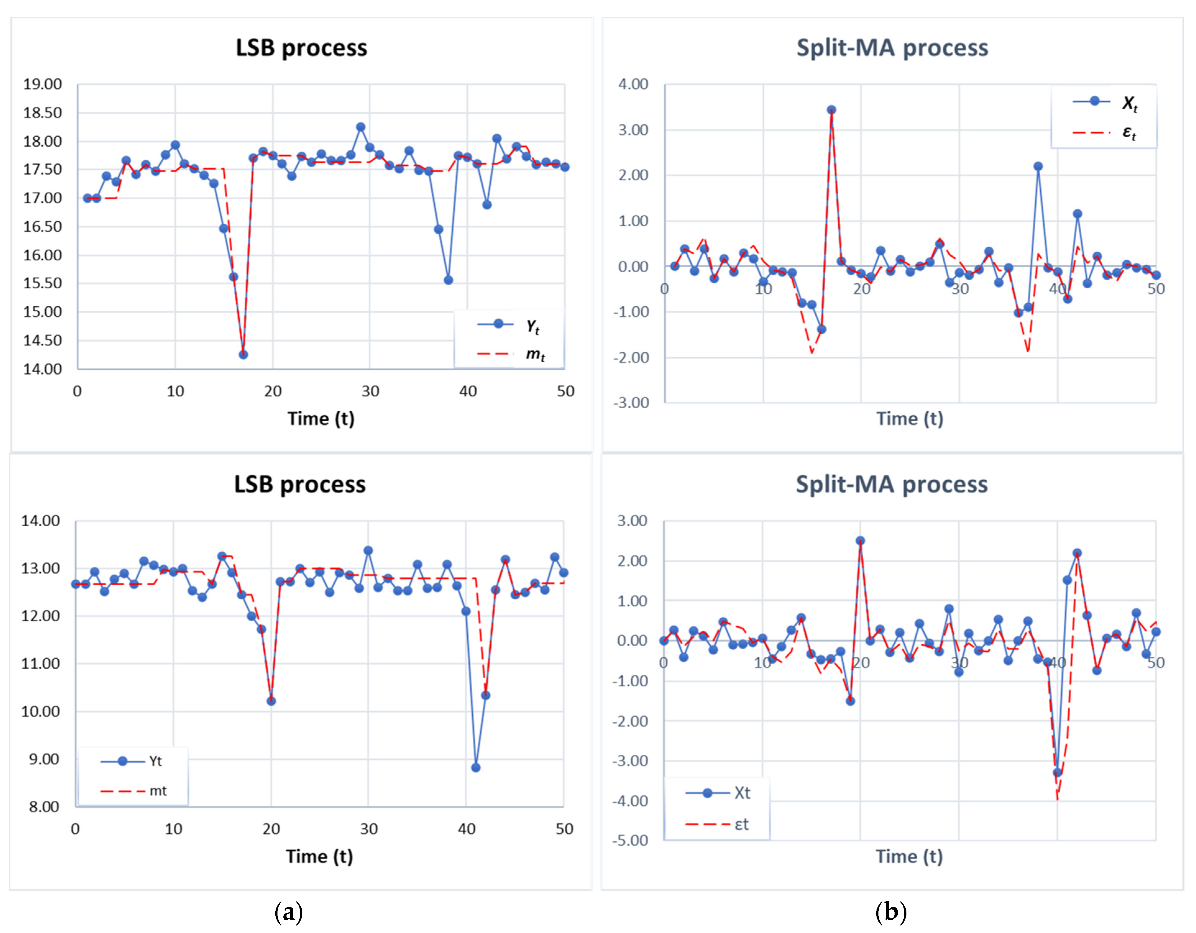
Figure 2 shows the realizations of all LSB time series obtained by Monte Carlo simulations. Note that non-stationary time series y t and m t (graphs on the left) can have very different trajectories, in contrast to realizations of the stationary series X t and ε t (graphs on the right).

3. Distributional Features of the LSB Process

Some important stochastic properties of LSB series, regarding their distributions and asymptotic behaviour, are discussed here. To this end, as mentioned earlier, the series X t plays a significant role due to its stationary quality. Using the method of characteristic functions (CFs), the basic stochastic properties of this series can be expressed in the following way.
Theorem 3. 
Let   X t   be the time series defined by Equations (8) and (9). Then, for any   x R   and   t = 0 , 1 , , T   , the CDF of the RVs   X t   is given by:
F X x P X t < x = 1 b c 2 F ε x + b c 4 G x ,
where   F ε x   is the CDF of the Laplacian distributed RVs   ε t   , given by Equation (4), and
G x 1 + s g n x 1 x λ + 1 exp x λ , x R .
Proof. 
To begin with, let us define the series of RVs ξ t = θ t ε t , t = 0 , 1 , , T . Thereby, the RVs ( θ t ) and ( ε t ) are mutually independent, so it follows:
E ξ t = E θ t E ε t = 0 , V a r ξ t = E θ t 2 E ε t 2 = 2 b c λ 2 .
It can easily be shown that it is C o v ξ t , ξ t + h = 0 , i.e., the RVs ξ t are uncorrelated for any h 0 . Using the conditional probabilities, for the CDF of the RVs ξ t one obtains:
F ξ x P ξ t < x = P ξ t < x θ t = 1 · P θ t = 1 + P ξ t < x θ t = 0 · P θ t = 0 = P ε t < x · P θ t = 1 + P x > 0 · P θ t = 0 = b c F ε x + 1 b c F 0 x ,
where F 0 x = I x > 0 is the CDF of the RV I 0 = a s 0 . According to this, the CF of the RVs ξ t is obtained as follows:
φ ξ u + e i u x F ξ d x = + e i u x b c F ε + 1 b c F 0 d x = b c φ ε u + 1 b c φ 0 u .
Here, φ ε u = 1 + λ 2 u 2 1 and φ 0 u 1 are, respectively, CFs of the RVs ε t and I 0 = a s 0 . Substituting these CFs into the previous equality gives:
φ ξ u = 1 + b c 1 1 + λ 2 u 2 1 .
According to this equality and Equation (9), as well as the result of using the partial decomposition of rational functions, for the CF of the RVs X t one obtains:
φ X u = φ ε u · φ ξ u = 1 b c 1 + λ 2 u 2 + b c 1 + λ 2 u 2 2 = 1 b c 1 + λ 2 u 2 + b c 4 1 1 + i λ u + 1 1 i λ u + 1 1 + i λ u 2 + 1 1 i λ u 2 = 1 b c 1 + λ 2 u 2 + b c 2 1 + λ 2 u 2 + b c 4 1 + 2 i λ u 2 2 + 1 2 i λ u 2 2 = 1 b c 2 1 + λ 2 u 2 + b c 4 ψ k λ u 2 + ψ k λ u 2 .
Here, ψ k u = 1 2 i u k / 2 are the CFs of RVs χ k 2 with chi-square distribution and k = 4 degrees of freedom (DF). According to Lévy’s correspondence theorem (see, c.f., [27]), the CDFs which correspond to CFs ψ k λ u / 2 and ψ k λ u / 2 are chi-square-based RVs λ χ k 2 / 2 and λ χ k 2 / 2 , respectively. By applying the well-known facts about χ k 2 distribution, these CDFs are, respectively,
G 1 x P λ 2 χ k 2 < x = P χ k 2 > 2 x λ = x λ + 1 exp x λ , x 0 1 , x > 0 ; G 2 x P λ 2 χ k 2 < x = P χ k 2 < 2 x λ = 1 x λ + 1 exp x λ , x 0 0 , x < 0 .
Note that the functions G 1 x and G 2 x satisfy the equality G x = G 1 x + G 2 x , where G x is the function given by Equation (11). Hence, by again applying the Lévy’s correspondence theorem to the last expression in (12), Equation (10) immediately follows. □
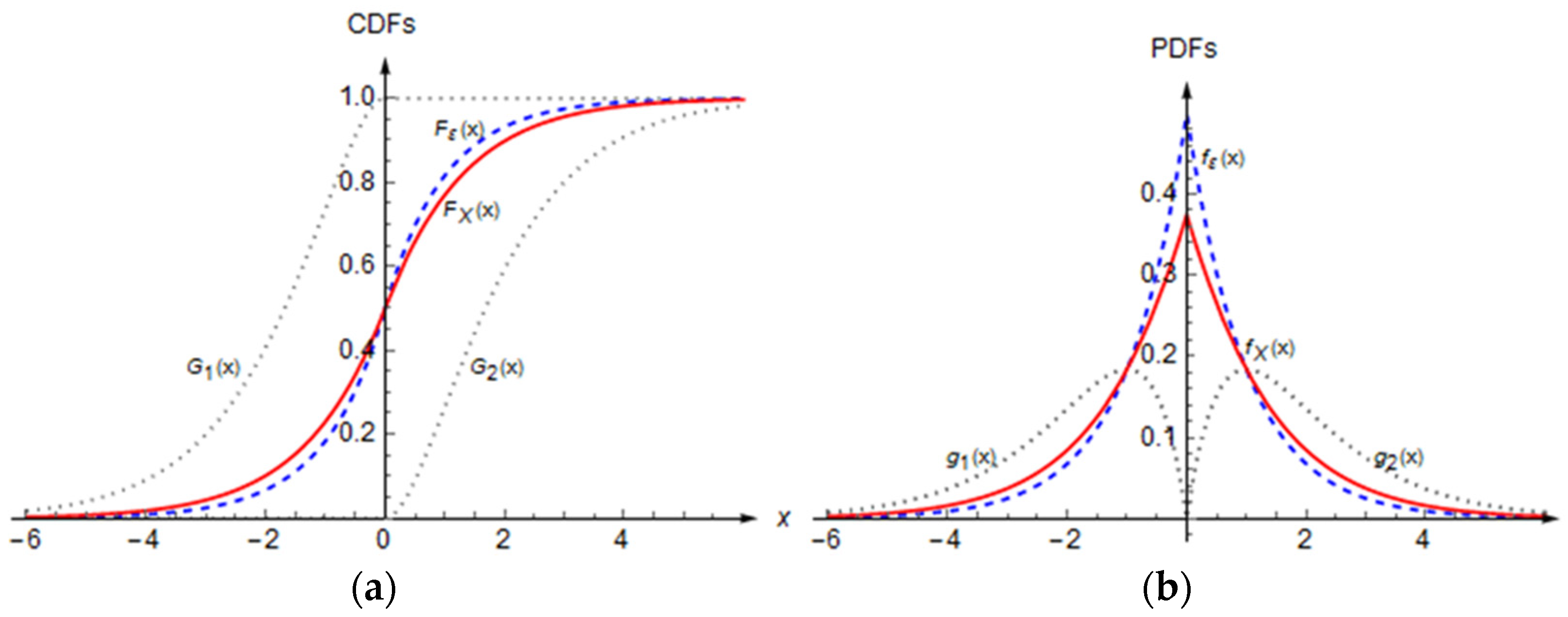
Remark 1. 
Let us emphasize that the function   G x   is not an ‘ordinary’ CDF, but the sum of two chi-square-based CDFs   G 1 x   and   G 2 x   , which can also be seen in the left plot in Figure 3. Furthermore, by differentiating Equation (10) when   x 0   , and after some computations, the probability density function (PDF) of the series   X t   can be obtained as follows:
f X x = 1 b c 2 d F ε x d x + b c 4 d G x d x = 1 2 λ exp x λ 1 + b c 2 x λ 1 .
Notice that PDF   f X x   differs from the PDF of the innovations   ε t   with respect to the last multiplicative term in Equation (13). Moreover, these PDFs become equal when   b c = 0 , and both are symmetric functions, as shown in the right-hand plots of Figure 3. ■
Using a similar procedure, the distributive properties of non-stationary LSB series m t and y t can be shown as follows.
Theorem 4. 
Let   y t   and   m t   be the time series defined by Equations (1) and (5), respectively, where   m 0 = a s μ c o n s t   . Then, for any   x R   and   t = 0 , 1 , , T , the CDFs of the series   m t   and   y t   are, respectively,
F m x , t P m t < x = t j = 1 1 b c F ε ( j ) x + b c F 0 x F μ x ,
F y x , t P y t < x = t j = 1 1 b c F ε ( j ) x + b c F 0 x F μ x F ε x ,
where is the convolution operator, and   F 0 x ,   F ε ( j ) x   are the CDFs of the RVs   I 0 , ε t , respectively. Additionally, the following convergences (in the distribution) hold when   T = + :
1 t m t d N 0 , 2 a c λ 2 , 1 t y t d N 0 , 2 a c λ 2 , t + .
Proof. 
Similarly to the previous theorem, let us introduce RVs η t = q t ε t , t = 0 , 1 , , T . It is easy to show that η t is a series of mutually uncorrelated RVs, with E η t = 0 , V a r η t = 2 a c λ 2 , where a c = E q t = P ε t 2 > c = 1 b c . Applying the conditional probabilities again, for the CDF of ( η t ) one obtains:
F η x P η t < x = P η t < x q t = 1 · P q t = 1 + P η t < x q t = 0 · P q t = 0 = P ε t < x · P q t = 1 + P x > 0 · P q t = 0 = a c F ε x + 1 a c F 0 x .
According to this CDF, the appropriate CF of the RVs η t can be obtained as follows:
φ η u = + e i u x F η d x = + e i u x a c F ε + 1 a c F 0 d x = a c φ ε u + 1 a c φ 0 u = 1 + a c 1 1 + λ 2 u 2 1 = 1 b c 1 + λ 2 u 2 + b c .
Now, by using Equation (5), for the CFs of the martingale means m t one obtains:
φ m u , t = φ μ u j = 0 t 1 φ η u = e i u μ 1 b c 1 + λ 2 u 2 + b c t ,
where φ μ u = e i u μ is CF of the RV m 0 = a s μ . According to Equation (17) and the correspondence theorem of Lévy [27], Equation (14) follows. In a similar way, according to Equation (1), the CFs of the series y t can be written as follows:
φ y u , t = φ m u · φ ε u = e i u μ 1 + λ 2 u 2 · 1 b c 1 + λ 2 u 2 + b c t .
From here, Equation (15) is immediately followed by reapplying the correspondence theorem of Lévy.
Let us now prove the second part of the theorem, that is, Equation (16). First, using previous Equations (17) and (18), for the CFs of RVs m t / t and y t / t , when t = 1 , 2 , , one obtains:
φ m u t , t = e i u μ / t 1 + a c t t + λ 2 u 2 1 t = e i u μ t 1 a c λ 2 u 2 t + λ 2 u 2 t , φ y u t , t = t e i u μ / t t + λ 2 u 2 1 + a c t t + λ 2 u 2 1 t = t e i u μ / t t + λ 2 u 2 1 a c λ 2 u 2 t + λ 2 u 2 t .
From here, taking the limit values, when t + and u R is a fixed (but arbitrary) value, the following is obtained:
lim t + φ m u t , t = lim t + φ y u t , t = e a c λ 2 u 2 .
Thus, obtained limit is the obvious the CF of the Gaussian distribution N 0 , 2 a c λ 2 , which confirms the convergences in (16). □
Remark 2. 
In the proofs of the previous two theorems, the uncorrelated series of RVs   ξ t   and   η t   can be interpreted as innovations with non-zero “optional” values. As the relation ξ t + η t = a s ε t   holds ,   it is sufficient to take only one of these two series for consideration. Moreover, it is easy to see that these RVs have the following CDFs:
F ξ x = b c F ε x + 1 b c F 0 x , F η x = 1 b c F ε x + b c F 0 x = F ε x + F 0 x F ξ x .
Obviously, both of these functions are continuous almost everywhere, with the only breaking point   x = 0   where ‘jumps’ of size   1 b c   and   b c   occur, respectively (for more details see Stojanović et al. [28,29]). For these reasons, the CDFs of the series   ξ t   and   η t   represent mixtures of the Laplacian and discrete distribution concentrated at zero, which we call the Contaminated Laplacian Distribution (CLD). This fact prevents the application of some of the standard procedures in the examination the properties of non-stationary series   y t   and   m t   .
On the other hand, asymptotic relations in Equation (16) show that even non-stationary time series   m t   and   y t   , obtained by non-Gaussian innovations   ε t   , one can generate series   m t / t   and   y t / t   , which will converge to Gaussian distribution when   t + . These facts are of practical importance when applying the LSB process and can be easily observed by the convergence of the appropriate CFs   φ m u / t , t   and   φ y u / t , t . As an illustration of this, convergences of the modulus of both of these CFs, for different time values, are shown in Figure 4. ∎
In the following, the asymptotic properties of some other time series, obtained by linear transformations of the non-stationary time series m t and y t are presented. It primarily refers to the possibility of finding their asymptotically normal (AN) distributions, and can be proven by the following proposition:
Theorem 5. 
Let us define, for an arbitrary α 1 , the α -mean time series:
M t ; α = 1 t α j = 1 t m j , Y t ; α = 1 t α j = 1 t y j ,
where y t and m t are the non-stationary time series given by (1) and (5), respectively. Then the following statements are valid:
(i)
When 1 α 3 / 2 , both series M t ; α and Y t ; α have an asymptotically normal distribution, i.e., the following relations, when t + , are valid:
M t ; α ~ N μ t 1 α , 2 a c λ 2 t 3 2 α 3 , Y t ; α ~ N μ t 1 α , 2 a c λ 2 t 3 2 α 3 .
(ii)
When α > 3 / 2 , both series M t ; α and Y t ; α are asymptotically vanishing, i.e.,
M t ; α d I 0 , Y t ; α d I 0 , t + .
Proof. 
First, we prove the statement of the theorem in the case of series M t ; α . According to the definition of series m t , given by Equation (5), the following is obtained:
M t ; α = 1 t α j = 1 t m j = 1 t α j = 1 t m 0 + k = 0 j 1 q k ε k = 1 t α t m 0 + j = 0 t 1 t j q j ε j = t 1 α m 0 + k = 1 t k t α η t k .
Therefore, the time series M t ; α is represented as the sum of uncorrelated RVs η t k , when k = 1 , , t . Applying the well-known features of the CFs, as well as the CF of the series η t , for the CFs of RVs M t ; α one obtains:
φ M ; α u , t = φ m u t α 1 , 0 k = 1 t φ η k u t α = e i u μ t 1 α k = 1 t 1 + a c t 2 α t 2 α + k 2 λ 2 u 2 1 .
From here, by taking the logarithm of the function φ M ; α u , t , the following function is obtained:
ψ M u , t , α ln φ M ; α u , t = i u μ t 1 α + k = 1 t f k u , t , α ,
where:
f k u , t , α ln 1 + a c t 2 α t 2 α + k 2 λ 2 u 2 1 = ln 1 a c k 2 λ 2 u 2 t 2 α + k 2 λ 2 u 2 .
After some computation, we find that:
f k 0 , t , α u = 2 a c k 2 λ 2 t 2 α u t 2 α + k 2 λ 2 u 2 t 2 α + 1 a c k 2 λ 2 u 2 u = 0 = 0 , 2 f k 0 , t , α u 2 = 2 a c k 2 λ 2 t 2 α t 4 α + a c 2 k 2 λ 2 t 2 α u 2 + 3 a c 1 k 4 λ 4 u 4 t 2 α + k 2 λ 2 u 2 2 t 2 α + 1 a c k 2 λ 2 u 2 2 u = 0 = 2 a c k 2 λ 2 t 2 α < 0 .
Thus, the functions f k u , t , α have a local maximum at the point u = 0 . By applying the Laplace approximation of functions f k u , t , α at u = 0 (see, c.f. [25,28]), it follows:
ψ M u , t , α = i u μ t 1 α + k = 1 t 2 f k 0 , t , α u 2 · u 2 2 + o k u 2 = i u μ t 1 α k = 1 t a c k 2 λ 2 t 2 α u 2 + o k t 2 α u 2 = i u μ t 1 α a c λ 2 u 2 t 2 α · t t + 1 2 t + 1 6 + o t 2 2 α u 2 .
Here o z denotes an infinitesimally small value of a higher order in relation to z , when z 0 . Taking the asymptotic value in the previous expression, when t + , gives:
ψ M u , t , α ~ i u μ t 1 α a c λ 2 t 3 2 α / 3 , 1 α 3 2 0 , α > 3 2 .
Substituting this expression in CFs φ M ; α u , t , it is easy to see that the first asymptotic relation in Equation (19) is valid.
The proof for the series Y t ; α can be conducted in an analogous manner. Using the previously proven facts and Equation (1), we find that:
Y t ; α = 1 t α j = 1 t m j + ε j = M t ; α + j = 1 t ε j t α = t 1 α m 0 + k = 1 t k t α η t k + k = 0 t 1 ε t k t α = t 1 α m 0 + ε t t α + k = 1 t 1 + k q t k ε t k t α .
Since ε t k , k = 0 , 1 , , t , are mutually independent RVs, the CFs of time series Y t ; α can be obtained, after some calculations, as follows:
φ Y ; α u , t = φ m u t α 1 , 0 φ ε u t α k = 1 t 1 a c φ ε u t α + a c φ ε k + 1 u t α = t 2 α e i u μ t 1 α t 2 α + λ 2 u 2 k = 1 t [ t 2 α t 2 α + λ 2 u 2   +   a c ( t 2 α t 2 α + λ 2 k + 1 2 u 2 t 2 α t 2 α + λ 2 u 2 ) ] = e i u μ t 1 α t 2 α t 2 α + λ 2 u 2 t + 1 k = 1 t 1 + a c t 2 α + λ 2 u 2 t 2 α + λ 2 k + 1 2 u 2 1 .
Based on this, and applying the same procedure as in the previous part of the proof, that is, by taking the logarithm of the function φ Y ; α u , t , and by expanding the function ψ Y u , t , α ln φ Y ; α u , t at u = 0 , we have:
ψ Y u , t , α = i u μ t 1 α + t + 1 ln t 2 α t 2 α + λ 2 u 2 + k = 1 t l n 1 + a c t 2 α + λ 2 u 2 t 2 α + λ 2 k + 1 2 u 2 1 = i u μ t 1 α + t + 1 ln 1 λ 2 u 2 t 2 α + λ 2 u 2 k = 1 t a c k 2 + 2 k λ 2 u 2 t 2 α + o k t 2 α u 2 = i u μ t 1 α λ 2 u 2 t + 1 t 2 α + λ 2 u 2 a c λ 2 u 2 t 2 α · t t + 1 2 t + 7 6 + o t 2 2 α u 2 .
Taking the asymptotic values, when t + , the following is obtained:
ψ Y u , t , α ~ i u μ t 1 α λ 2 u 2 t 1 2 α + a c t 2 α + a c t 3 2 α 3 , 1 α 3 2 0 , α > 3 2 .
Replacing this expression in the CFs φ Y ; α u , t , the theorem is completely proven. □
Remark 3. 
As with the GSB process, the case α = 3 / 2 is of special interest in the previous theorem. Asymptotic relations (19) then give:
1 t 3 / 2 j = 1 t m j d N 0 , 2 a c λ 2 3 , 1 t 3 / 2 j = 1 t y j d N 0 , 2 a c λ 2 3 , t + .
The convergences (21), as in the case of GSB process, we called the central limit theorems (CLTs) for the LSB process. ■

4. Procedures for Parameter Estimation

In this section, we consider the estimations of the (unknown) parameters of the LSB process, that is the critical value c , the scale parameter λ , and the mean value μ . In order to estimate the first parameter c , it should be emphasized that a series of increments X t , as the only observable and stationary series of the LSB process, will be used. As has already been pointed out, this series is close to standard, linear MA models, but with Laplacian distributed innovations ε t . For these reasons, the estimation procedures like those used for the mentioned time series will be used here. However, the specificity of the series X t requires some additional estimation procedures, as well as examination of the quality of the obtained estimators.

4.1. Moments-Based Estimators

According to Theorem 2, the first correlation of the series X t is as follows:
ρ X 1 = b c 1 + b c , 0 < b c < 1 ,
and solving on b c , the estimated value of this parameter is obtained:
b ~ c = ρ ^ X 1 1 + ρ ^ X 1 .
Note that it is here:
ρ ^ X 1 = t = 1 T X t X t 1 t = 1 T X t 2 1
the sample autocorrelation of the Split-MA(1) process X t . According to Equation (22), it is easy to see that b ~ c is the appropriate estimate if and only if
0 < b ~ c < 1 0.5 < ρ ^ X 1 < 0 .
Using the estimator b ~ c , the squared scale parameter λ 2 can be estimated by applying the equality:
V a r X t = E X t 2 = 2 λ 2 b c + 1 .
Applying Theorem 2 again, as well as the sample variance for X t , we get the estimator:
λ ~ 2 = 1 2 T b ~ c + 1 t = 1 T X t 2 .
It is worth pointing out that in Stojanović et al. [21] it is proven that the estimators b ~ c and λ ~ 2 are strictly consistent if innovations ε t have a continuous distribution. Moreover, these estimators are asymptotically normal (AN) in the case of symmetrically distributed RVs ε t . Note that both conditions are satisfied for Laplace innovations ε t and, hence, it follows:
Theorem 6. 
The estimators b ~ c and λ ~ 2 , given by Equations (22) and (23), respectively, are strictly consistent estimates for the parameters b c and λ 2 , i.e.,
b ~ c a s b c , λ ~ 2 a s λ 2 , T + .
In addition, b ~ c and λ ~ 2 are asymptotically normal estimators for b c and λ 2 , respectively, i.e.,
T b ~ c b c d N 0 , V ~ 1 , T λ ~ 2 λ 2 d N 0 , V ~ 2 , T + ,
where:
V ~ 1 = 1 + b c 2 1 + 7 b c 3 b c L + b c , V ~ 2 = 4 λ 4 5 + 20 b c + 2 b c L 3 b c 2 V ~ 1 , L = 1 2 λ 2 E θ t ε t 1 2 = 1 2 λ 2 E θ t 2 ε t 1 2 = 1 c λ c 2 λ 2 + c λ + 1 .
Proof. 
According to Theorem 2, X t is a stationary series of RVs and its spectral density is:
s X ω = 1 2 π γ X 1 e i ω + γ X 0 + γ X 1 e i ω = λ 2 π 1 2 b c cos ω + b c ,
where γ X h = C o v X t , X t + h = E X t X t + h is the covariance function of X t . Obviously, the function s X ω is continuous at the point ω = 0 , so X t is also an ergodic series of RVs. Thus, by applying the mean ergodic theorem (see, c.f. [30], pp.131), for any h 0 , one obtains:
1 T t = 1 T X t X t + h a s γ X h , T + .
Hence, by applying the convergence (26), when h = 0 , 1 , to the estimators b ~ c and λ ~ 2 , given by Equations (22) and (23), respectively, the almost certain convergence in (24) is easily obtained.
Now, let us define series Z t = X t X t + 1 , t = 0 , 1 , , T 1 , which has 1-dependent property (see, c.f. Definition 6.3.1 in [31], pp.245). Obviously, the series Z t is also stationary and ergodic, with:
E Z t = C o v X t , X t + 1 = γ X 1 = 2 b c λ 2 .
According to the Cauchy–Swartz and Minkowski inequalities, it follows:
E Z t γ X 1 3 E Z t 3 1 / 3 + 2 b c λ 2 3 < + ,
and by applying the Hoeffding–Robbins theorem [32], we have:
T Z t γ X 1 = T 1 2 t = 1 T X t X t + 1 + 2 b c λ 2 d N 0 , A , T + .
Here, after some computations, one obtains:
A = V a r Z t + 2 C o v Z t , Z t + 1 = E X t 2 X t + 1 2 + 2 E X t X t + 1 2 X t + 2 3 γ X 2 1 = 4 λ 4 1 + 7 b c + b c L 16 λ 4 b c L + 12 λ 4 b c 2 = 4 λ 4 1 + 7 b c 3 b c L + b c .
In addition, by again applying the mean ergodic theorem, i.e., Equation (26) when h = 0 , it follows:
1 T t = 1 T X t 2 a s E X t 2 = 2 λ 2 b c + 1 , T + .
Thus, the convergences (27) and (28) imply:
T ρ ^ X 1 ρ X 1 d N 0 , V 0 , T + ,
wherein:
V 0 = A γ X 2 0 = 1 + 7 b c 3 b c L + b c 1 + b c 2 .
Finally, according to the continuity of convergence in distribution (see, c.f. [33], pp.118), it follows:
T b ~ c b c d N 0 , V ~ 1 , T + ,
wherein:
V ~ 1 = d ρ X 1 d b c 2 V 0 = 1 + b c 4 V 0 .
In that way, the first convergence in (25) is proved.
To prove the second convergence in (25), note that series X t 2 is also 1-dependent. According to previous mentioned inequalities, as well as Theorem 2, one obtains:
E X t 2 γ X 0 3 E X t 6 1 / 3 2 λ 2 b c + 1 3 < + .
Thus, by applying again the Hoeffding–Robbins theorem [32], we get:
T 1 2 t = 1 T X t 2 2 λ 2 b c + 1 d N 0 , D , T + ,
where, after some computations, one obtains:
D = V a r X t 2 + 2 C o v X t 2 , X t + 1 2 = 4 λ 4 5 + 20 b c + 2 b c L 3 b c 2 .
Finally, according to the first almost certain convergence in (24), as well as the previously obtained convergence (30), it follows:
T λ ~ 2 = 1 2 T b ~ c + 1 t = 1 T X t 2 d N λ 2 , V ~ 2 , T + ,
where V ~ 2 = D / V ~ 1 . Thus, the second convergence in (25) is obtained. ■
Remark 4.
Using the estimators b ~ c and λ ~ 2 , the appropriate estimator of the critical value c = c ~ can be easily obtained as a solution to the equation:
P ε t 2 c = b ~ c ,
or, equivalently,
F ε c F ε c = 2 F ε c 1 = b ~ c c ~ = F ε 1 b ~ c + 1 2 2 .
Here, F ε x is the CDF of the Laplacian innovations ε t , given by Equation (4), and we also note that in Equation (31) the property of symmetry of its distribution is used. It is also noticeable that, from the fact that c ~ is a continuous function of the estimator b ~ c , the strong consistency and AN property of this estimator follows (see, c.f. [33], pp. 24).

4.2. Gauss–Newton and Maximum Likelihood Estimators

It is worth pointing out that b ~ c and λ ~ 2 are not the most efficient estimators for b c and λ 2 . In order to obtain more efficient estimators for the observed parameters, similarly to the case of the GSB process (see, c.f. [21,25]), the so-called modified Gauss–Newton method of parameter estimation of nonlinear functions can be used. First, we can write Equation (9) as:
ε t = X t + θ t 1 ε t 1 , t = 1 , , T ,
or, in the functional form,
ε t X , θ = X t + θ t 1 ε t 1 X , θ .
Let b ~ c be the estimated value of the parameter b c , obtained by the previously described procedure. According to this, for each t = 1 , 2 , , T , we can recursively compute:
θ ~ t I ε t 1 2 X , θ ~ c ~ , ε t X , θ ~ X t + θ ~ t 1 ε t 1 X , θ ~ ,
with the previously mentioned initial values θ ~ 0 = 1 , ε 0 X , θ ~ = ε 1 X , θ ~ = 0 . Additionally, if we define a series of RVs:
W t X , θ = θ t W t 1 X , θ + ε t 1 X , θ ,
where t = 1 , 2 , , T , and W 0 X , θ ~ = 0 , it is obvious that RVs W t X , θ are F t 1 adapted, and thus independent of ε t and θ t + 1 . Furthermore, according to mentioned properties of RVs θ t and ε t , it follows that W t X , θ is a stationary and ergodic series of RVs with:
E W t X , θ = 0 , V a r W t X , θ = E W t X , θ 2 = 2 λ 2 1 b c ,
and correlation function ρ W h = b c h , h = 0 , ± 1 , Now, using a procedure similar to the one in Lawrence and Lewis [34], we define the so-called residual series:
R t X , θ = W t X , θ b c W t 1 X , θ .
It can be shown easily that R t X , θ are also F t 1 adapted, but mutually non-correlated RVs (see, c.f. Jovanović et al. [25]). Thus, Equation (34) represents a linear autoregressive (AR) process W t X , θ with innovations R t X , θ . From here, by applying the usual regression procedure, another estimator of the unknown, threshold parameter b c 0,1 can be obtained by the equality:
b ^ c = t = 0 T 1 W t X , θ ~ W t + 1 X , θ ~ t = 0 T 1 W t 2 X , θ ~ 1 ,
where, according to Equations (33) and (34),
W t X , θ ~ W t X , θ θ = θ ~ = θ ~ t W t 1 X , θ ~ + ε t 1 X , θ ~ , R t X , θ ~ R t X , θ θ = θ ~ = W t X , θ ~ b c W t 1 X , θ ~ .
As in the case of previous estimators, the estimator b ^ c gives the estimator of critical value c = c ^ as a solution of the equation:
P ε t 2 c = b ^ c c ^ = F ε 1 b ^ c + 1 2 2 .
Notice that using the previously obtained estimators b ~ c (as well as b ^ c ), that is, the modelled values of innovations ε t , defined by Equation (32), the scale parameter λ can be estimated. It is well-known that for the Laplace innovations ε t the most efficient estimates are obtained by using the maximum likelihood (ML) estimators (see, c.f. [35,36]). In the case of our LSB process, the ML estimator can be obtained according to Equations (1) and (2), that is, based on the maximization of the log-likelihood function:
l y 1 , , y T ; λ = ln t = 1 T 1 2 λ exp y t m t λ = T ln 2 λ 1 λ t = 1 T ε t X , θ ~ .
By solving the equation l y 1 , , y T ; λ / λ = 0 and using Equation (32), the estimator of scale parameter λ is obtained as the mean absolute deviation (MAD):
λ ^ = 1 T t = 1 T ε t X , θ ~ .
Strict consistency and AN of the estimates b ^ c and λ ^ can be proven as follows:
Theorem 7. 
Estimators b ^ c and λ ^ , defined by Equations (34) and (36), respectively, are strictly consistent estimators for the parameters b c and λ , i.e.,
b ^ c a s b c , λ ^ a s λ , T + .
Moreover, b ^ c and λ ^ are asymptotically normal estimators for b c and λ , respectively, i.e.,
T b ^ c b c d N 0 , 1 b c 2 , T λ ^ λ d N 0 , λ 2 , T + .
Proof. 
According to definitions of the residuals ( R t ( X , θ ~ ) ) and the estimator b ^ c , given by Equations (34) and (35), respectively, we obtain:
b ^ c b c = t = 0 T 1 W t X , θ ~ W t + 1 X , θ ~ b c t = 0 T 1 W t 2 X , θ ~ t = 1 T W t 2 X , θ ~
= t = 0 T 1 W t X , θ ~ R t + 1 X , θ ~ t = 0 T 1 W t 2 X , θ ~ .
Similarly to the previous theorem, it can be shown that ( W t ( X , θ ~ ) ) , ( R t ( X , θ ~ ) ) , and ( ε t ( X , θ ~ ) ) are stationary and ergodic time series. Thus, by applying the mean ergodic theorem, it follows:
1 T t = 0 T 1 W t X , θ ~ R t + 1 X , θ ~ a s E W t X , θ ~ R t + 1 X , θ ~ = 0 , T + , 1 T t = 0 T 1 W t 2 X , θ ~ a s E W t 2 X , θ ~ = 2 λ 2 1 b c , T + ,
1 T t = 0 T 1 ε t X , θ ~ a s E ε t X , θ ~ = λ , T + .
These convergences obviously imply the almost certain convergences in Equation (38).
Furthermore, according to Equation (40), in the following decomposition one obtains:
T b ^ c b c = T 1 2 M T 1 T 1 W T 1 ,
wherein:
M T 1 t = 0 T 1 W t X , θ ~ R t + 1 X , θ ~ , W T 1 t = 0 T 1 W t 2 X , θ ~ .
As for each t = 1 , 2 , , T ,
E M t F t 1 = M t 1 + W t X , θ ~ E R t + 1 X , θ ~ = M t 1 ,
the series M t is a martingale. Applying Billingsley’s CLT for martingales [37], we get:
T 1 2 M T 1 d N 0 , D 1 ,
wherein, according to Equation (34),
D 1 = E W t X , θ ~ R t + 1 X , θ ~ 2 = E W t 2 X , θ ~ E W t + 1 X , θ b c W t X , θ 2 = 2 λ 2 1 b c E W t + 1 2 X , θ ~ 2 b c W t X , θ W t + 1 X , θ + b c 2 W t 2 X , θ ~ = 2 λ 2 1 b c 2 λ 2 1 + b c 2 1 b c 2 b c C o v W t X , θ , W t + 1 X , θ = 2 λ 2 1 b c 2 λ 2 1 + b c 2 1 b c 4 λ 2 b c 2 1 b c = 4 λ 4 1 + b c 1 b c .
On the other hand, the almost certain convergence in Equation (41) is the same as:
T 1 W T 1 a s 2 λ 2 1 b c , T + .
Thus, the convergences (42) and (43) give the first convergence in (39). Finally, according to Equation (33), and after some computations, one obtains:
V a r λ ^ = 1 T 2 t = 1 T E ε t 2 X , θ ~ λ 2 = 1 T E W t + 1 X , θ θ t + 1 W t X , θ 2 λ 2 = 1 T E W t + 1 2 X , θ 2 E θ t + 1 W t + 1 X , θ W t X , θ + E θ t + 1 W t 2 X , θ λ 2 = 1 T 2 λ 2 1 + b c 1 b c 2 E θ t + 1 θ t + 1 W t X , θ + ε t X , θ W t X , θ λ 2 = 1 T 2 λ 2 1 + b c 1 b c 2 E θ t + 1 W t 2 X , θ λ 2 = 1 T 2 λ 2 1 + b c 1 b c 4 λ 2 b c 1 b c λ 2 = λ 2 T ,
and the second convergence in (39) immediately follows □
Remark 5. 
Similarly to Theorem 6, the estimator c ^ , defined by Equation (36), is a continuous function of b ^ c . Thus, the strong consistency and AN properties of c ^ are also valid. Additionally, based on the scale parameter estimator λ ^ given by Equation (37), the estimator λ ^ 2 can be defined. It is also strictly consistent and AN but, at the same time, the most efficient estimator for the parameter λ 2 . Namely, by applying the continuity of the convergence in distribution [33], (pp. 118), it follows that:
T λ ^ 2 λ 2 d N 0 , V ^ 2 , T + ,
where V ^ 2 = λ 2 2 λ 2 = 4 λ 4 . Thus, the variance of the estimator λ ^ 2 is 4 λ 4 / T and it is the minimum of the variance for the unbiased estimator of the parameter λ 2 , obtained from Rao–Cramér’s inequality (see, c.f. [35,36]). In that way, for the previously defined estimators, inequalities:
V ^ 1 b c V ~ 1 b c ,   V ^ 2 λ 2 V ~ 2 b c , λ 2
hold, where we denoted V ^ 1 b c = 1 b c 2 . This means that b ^ c and λ ^ 2 are more efficient estimators than b ~ c and λ ~ 2 , respectively, which can also be seen inFigure 5, where asymptotic variances of these estimators are shown.

4.3. Estimators of the Mean Value

In the last part of this section, we consider estimators for the mean value of the LSB process μ = E y t . For this aim, the sample mean of series is usually used y t :
μ ~ = y T = 1 T t = 1 T y t ,
which is an unbiased estimator, that is, E ( μ ~ ) = E y T = μ , but its variance is unbounded. To prove this fact, we use the α -mean series Y T ; α , defined in Theorem 5, in the case where α = 1 . Then, the estimator μ ~ can be represented as a sum of uncorrelated RVs:
μ ~ = m 0 + 1 T k = 1 T 1 + k q T k ε T k + ε T ,
and using the same procedure as in Theorem 5, the variance of μ ~ is as follows:
V ~ V μ ~ = 2 a c λ 2 T 3 + O T 1 + , T + .
Let us emphasize that the variance V ~ = V μ ~ is asymptotically equal to that in Equation (19), when α = 1 , as expected.
In order to obtain a more efficient estimator for the parameter μ , a sample mean of the mean series y t , when t = 1 , , T , can be taken, i.e.,
μ ^ = 1 T t = 1 T y t = 1 T t = 1 T ω t y t ,
where ω t H T H ( t 1 ) and H t j = 1 t j 1 , t = 1 , , T are the harmonic numbers, with H 0 = 0 . The estimator μ ^ is also unbiased for the parameter μ , but its weights are more pronounced at the ‘older’ time points of the realization of the series y t . This is consistent with the fact that the covariances of RVs y t depend on these ‘older’ time indices. For these reasons, the estimator μ ^ is more efficient than μ ~ , which can be shown using a procedure similar to that of Jovanović et al. [25]. First, we represent estimator μ ^ as a sum of uncorrelated RVs:
μ ^ = 1 T m 0 t = 1 T ω t + j = 0 T 1 q j ε j t = j + 1 T ω t + t = 1 T ω t ε t ,
and after some computations (see, for more detail [25]), the variance of μ ^ can be obtained as follows:
V ^ V μ ^ = 2 a c λ 2 H 2 T + o H 2 T + , T + .
In this way, it can be seen that the asymptotic variance V ^ = V μ ^ is also unbounded, but is asymptotically smaller than V ~ = V μ ~ , because:
lim T + V μ ^ V μ ~ = lim T + H 2 T T = 0 .
Thus, the estimator μ ^ is (asymptotically) more efficient than μ ~ .

5. Numerical Simulations of the LSB Estimators

In this section, the parameter estimation procedures of the LSB model are discussed, where N = 1500 Monte Carlo simulations of the basic LSB series are generated, of the length T = 1000 . At the same time, the main goal is to examine the quality of previously proposed estimators, that is, their asymptotic properties, which were analysed and shown in the previous section. To this end, appropriate estimation errors and normality testing procedures are also used. The summarized values of the estimated parameters, i.e., the mean (Mean), minimum (Min.), and maximum (Max.), as well as the corresponding mean square estimated errors (MSEE), are shown in the left part of Table 1. In addition, the obtained estimates were tested for their AN properties using Anderson–Darling and Cramér–von Mises normality tests. The appropriate test statistics (denoted by AD and W, respectively), as well as their p -values, were computed using the R-package “nortest” [38] and are presented in the right part of Table 1.
Based on these obtained estimates, it is evident that almost all of them have the AN property, which is also confirmed by the previous theoretical results. It is worth pointing out that even the estimates of the mean values μ ~ and μ ^ , obtained by the realizations of the non-stationary series y t , have the AN properties. This is already explained by the theoretical findings provided by Theorems 4 and 5, which describe the AN properties of this series. Therefore, the effectiveness of both of these estimators due to their non-stationarity is not pronounced and, due to unlimited variance, there are a wide range of obtained estimated values. On the other hand, we note that the AN property is not particularly emphasized in the case of estimates of the critical value ( c ) . This is a consequence of the three-step procedure for estimating this parameter, because the estimates of the parameter c are obtained after the estimates of the parameters b c and λ have been computed. Nevertheless, it is clear that, in accordance with the previous theoretical findings, first of all in Theorem 7, the estimate c ^ is more efficient and has a more pronounced AN property than estimate c ~ .
Finally, in the case of estimates of the scale parameter ( λ ) , their efficiency and AN properties are clearly visible. At the same time, it should be noticed that the moment-based estimate λ ~ has a somewhat slower efficiency and AN property compared to the ML estimate λ ^ , obtained using Equation (37) and the modelled innovations ε t . This is fully consistent with the previously explained theoretical findings, that is, the definitions of both of these two estimates, as well as Theorems 6 and 7. Some visual confirmation of these facts can be seen in Figure 6, where the histograms of the frequency distribution of the obtained estimates are shown. Thus, for instance, in all cases (with the exception c ~ ) the presence of AN properties clearly can be observed, as well as the efficiency of the obtained estimates.

6. Application in Dynamic Analysis of the World Oil and Gas Market

In the following, the application of the LSB process in the dynamic analysis of prices and trading volumes of crude oil and natural gas on the world market is considered. We emphasize that the temporal dynamics of these two energy sources is of particular importance, and they are greatly influenced by global external factors, such as, for instance, the recent COVID-19 pandemic and the war in Ukraine. Precisely for these reasons, it can be assumed that all of these factors cause permanent and pronounced fluctuations in the dynamics of the price and trading volume of these two energy products, which can be seen in the following Figure 7. As mentioned in the introduction, it will be shown here that the LSB process can be an appropriate stochastic model for describing dynamics of these kinds. To this end, based on official data from the National Association of Securities Dealers Automated Quotations (NASDAQ) Stock Market [39], we observed daily changes in crude oil prices and trading volumes (in US dollars per barrel) and natural gas (in US dollars per cubic meter) from 2 April 2018 to 31 March 2023.
In this way, time series of real-world data of length T = 1261 were obtained, and their main statistical indicators can be seen in the following Table 2. Based on these, it can be easily concluded that in both cases there are pronounced and permanent fluctuations. For example, the average price of crude oil is (approximately) 62.57 US dollars per barrel. However, it varies from 9.06 US dollars (on 21 April 2020, just over a month after the official announcement of the COVID-19 pandemic), all the way to 123.7 US dollars (on 8 March 2022, a few weeks after the start of the war in Ukraine). Let us notice that the price of natural gas also has pronounced price ranges, although less pronounced than in the case of the price of crude oil.
Note that in addition to the basic financial data (price and volumes of trading), Table 2 also shows descriptive statistics of the so-called log-volumes. They represent an aggregate financial indicator, obtained as a natural logarithm of the total monetary value of trading volumes, i.e.,
y t ( j ) : = ln P t j · V t j , t = 0 , 1 , , T j , j = 1 , 2 .
Here, P t 1 and V t 1 are, respectively, the price and trading volumes of crude oil, and P t 2 and V t 2 are the price and trading volumes of natural gas, observed at some point in time t = 1 , 2 , , T . As is stated in two studies [40,41], the usage of log-volumes changes the interpretation of activity shocks because unexpected values are not affected by the growth trend in their dynamics. In addition, the variance of log-volatility shocks is then more uniform across the sample (that is, over the timeline of the observed data). This can also be seen through the sample variance and standard deviation of both observed log-volume series, which are shown in Table 2. Additionally, the corresponding Split-MA(1) processes for these series are as follows:
X t ( j ) y t j y t 1 j = ln P t j P t 1 j + ln V t j V t 1 j , t = 1 , , T , j = 1 , 2 ,
i.e., they represent the sum of the log-returns of prices and trading volumes.
We further consider the possibility of using the LSB process as a suitable stochastic model of logarithmic volume dynamics. To that end, the basic LSB series, i.e., realizations of log-volumes of crude oil and natural gas, will be referred to as Series A and Series B, respectively. According to these, as well as the results of using Equations (1) and (5), the martingale means ( m t j ) and innovations ( ε t ( j ) ) can be obtained by iterative procedure:
ε t j = y t j m t j , m t j = m t 1 j + ε t 1 j I ε t 2 j 2 c ~ ,
where j = 1 , 2 and c ~ is the estimated critical value, obtained by using Equation (31). As initial values in (47), as before, we have taken ε 0 ( j ) = ε 1 ( j ) = 0 , as well as m 0 ( j ) = y 0 ( j ) = μ ^ , j = 1 , 2 . The estimated values of basic statistical indicators of the increment series ( X t ( j ) ) , j = 1 , 2 , as well as two modelled series, martingale means ( m t j ) , j = 1 , 2 , and innovation series ( ε t ( j ) ) , j = 1 , 2 , are presented in the following Table 3.
Based on the obtained estimated parameter values, certain observations can be made, which also derive from previously obtained theoretical results. Note first that the average values of log-volumes are “close” to the average values of martingale means, and that is consistent with equality E y t = E m t . Moreover, both series A and B have other similar statistical indicators (variance or standard deviation, for example), which indicates a certain similarity in their dynamics and other stochastic characteristics. This can be seen by comparing statistical indicators of the increments ( X t ( j ) ), j = 1 , 2 , and the innovation series ( ε t j ), j = 1 , 2 . It is noticeable that the sample means of both series are close to zero, that is, they have the property of symmetry of their empirical distributions. Finally, it is worth pointing out that both series ( ε t j ), j = 1 , 2 , have the estimated values of kurtosis K j 6 , j = 1 , 2 , which could indicate their suitability for stochastic modelling with the Laplace distribution.
In the following, using the estimation procedure described in the previous section, the parameters of both real-world time series can be estimated, assuming that their dynamics are subjected to the LSB model. Table 4 shows the estimates obtained by applying the above-mentioned procedures, that is, two kinds of parameter estimates of the LSB model. Additionally, some other estimates, such as the first-order sample correlation ρ ^ X ( 1 ) and the estimates of the threshold parameter b c , are shown. Let us notice that the condition 0.5 < ρ ^ X 1 < 0 is satisfied in both series cases, which enables the estimation of the parameter b c .
As has already been pointed out, the values of the modelled series ( m t j ) and ( ε t ( j ) ) were computed by using the most robust estimators of the LSB process c ^ , μ ^ , σ ^ 2 . The agreement between the modelled and actual data can be seen in Figure 8a, where in addition to the observed log-volume values ( y t ( j ) ), the modelled martingale mean values ( m t ( j ) ) are shown. At the same time, the agreement between the increment series ( X t ( j ) ) and innovations ( ε t ( j ) ) is shown in Figure 8b. It is worth noting that high correlations between the actual and modelled time series are clearly observable, which can also be explained by the theoretical findings presented in Section 2. Namely, the martingale means ( m t ( j ) ) are equal to the log-volumes in cases when there were no pronounced fluctuations of the series ( y t ( j ) ) in the previous time period. On the other hand, if emphatic fluctuations occur, the values of the series ( m t ( j ) ) and ( y t ( j ) ) become different, and the resulting deviations indicate the existence of significant fluctuations and potential risk in the market. Similarly, if at some point in time point’s innovation series ( ε t j ) has a pronounced fluctuation, the next value of ( ε t j ) will be equal to increments ( X t ( j ) ). It is obvious that the agreement of realizations between these time series is better if, in addition to permanent and emphatic fluctuations of ( ε t ( j ) ), the critical value c is relatively small.
Notice that the CDFs and PDFs of the series ( X t j ), j = 1 , 2 can be obtained by using the results given in Theorem 3, that is, Equations (10) and (13), respectively. The above plots in Figure 9 show fitted PDFs of both empirical distributions of the series ( X t j ), j = 1 , 2 . Finally, using the results of Theorem 4, that is, Equation (15), the fitted CDFs H t x of the log-volumes ( y t ( j ) ) can be obtained by the iterative procedure:
H t ( j ) x H t 1 j F η x = + H t 1 j x u F η d u , t = 1 , 2 , , T ,
where:
H 0 j x F μ F ε x = + F μ x u F ε d u = + I x u > μ f ε u d u = x μ f ε u d u = F ε x μ .
From here, by differentiating the CDFs obtained using Equation (48), the corresponding PDFs of the log-volumes ( y t ( j ) ) can also be easily computed. Therefore, due to the non-stationarity, these PDFs are dependent on the time argument t . The graphs below in Figure 9 show the theoretical PDFs of the series ( y t ( j ) ), obtained by using the numerical procedure in the R-package “distr” [42]. The PDFs of the length t < T = 1261 are shown with dashed lines, and the PDFs of the length T = 1261 are shown with a solid line.

7. Conclusions

The main stochastic properties of the Laplacian Split-BREAK (LSB) process are presented here, along with the investigation of the asymptotic properties of the corresponding LSB series, as well as the procedures for estimating their parameters. It is useful to point out that one of the advantages of this stochastic model, as in the case of the Gaussian Split-BREAK (GSB) process, is that it enables the usage of appropriate stationary and non-stationary components, which provide different procedures for estimating its unknown parameters. At the same time, of particular importance is the asymptotic behaviour of LSB series. This is considered as well as the obtained parameter estimators.
Let us point out that one of the important features of the LSB process, as well as the class of STOPBREAK-based processes in general, is the ability to “remove” the sharp boundary between stochastic processes with permanent shocks and those in which they remain transient. Therefore, these stochastic processes can vary between different well-known non-linear stochastic models (see, for more details, Stojanović et al. [23,24]). For instance, the LSB process can vary from an IID (white noise) series, for a larger critical value of reaction c , to a random walk process, as c approaches zero.
In addition, some of the possibilities of applying the LSB process in modelling dynamics of the real-world series with emphasized and persistent fluctuations are also described. This provides opportunities for potential future research based on the various kinds of Split-BREAK processes. At the same time, it is worth pointing out that the dynamic analysis of log-volumes, as composite time series, may represent a certain limitation, due to a possibility of omitting some other characteristics of the oil and gas market.

Author Contributions

Conceptualization, V.S.S. and H.S.B.; methodology, V.S.S. and H.S.B.; software, V.S.S.; validation, E.L. and I.B.; formal analysis, V.S.S. and H.S.B.; data curation, V.S.S. and I.B.; writing---original draft preparation, V.S.S., H.S.B., and E.L.; writing---review and editing, E.L. and I.B.; visualization, V.S.S. and H.S.B.; supervision, V.S.S. and H.S.B.; project administration, E.L. and I.B. All authors have read and agreed to the published version of the manuscript.

Funding

This research received no external funding.

Data Availability Statement

Official data on prices and trading volumes on the Oil and Gas World market can be found on the website https://nasdaq.com.

Conflicts of Interest

The authors declare no conflict of interest.

Abbreviations

The following abbreviations are used in this manuscript:
AD testAnderson–Darling test (statistics)
ANAsymptotic Normality
AR processAutoregressive process
CDFCumulative Distribution Function
CFCharacteristic Function
CLDContaminated Laplacian Distribution
DFDegrees of Freedom
GSB processGaussian Split-BREAK process
IIDIndependent Identical Distributed
LSB processLaplacian Split-BREAK process
MA processMoving Average process
ML methodMaximum Likelihood method
MSEEMean Square Estimated Error
NASDAQNational Association of Securities Dealers Automated Quotations
PDFProbability Density Function
RVRandom Variable
Split-MA processSplitting Moving Average process
STOPBREAKStochastic Permanent Breaking
W testCramér–von Mises test (statistics)

References

  1. Hardouvelis, G.A.; Kim, D. Margin Requirements, Price Fluctuations, and Market Participation in Metal Futures. J. Money Credit Bank. 1995, 27, 659–671. [Google Scholar] [CrossRef]
  2. Fatás, A. Endogenous Growth and Stochastic Trends. J. Monet. Econ. 2000, 45, 107–128. [Google Scholar] [CrossRef] [Green Version]
  3. Chang, Y.; Schorfheide, F. Labor-Supply Shifts and Economic Fluctuations. J. Monet. Econ. 2003, 50, 1751–1768. [Google Scholar] [CrossRef]
  4. Artis, M.J.; Hoffmann, M. Financial Globalization, International Business Cycles and Consumption Risk Sharing. Scand. J. Econ. 2008, 110, 447–471. [Google Scholar] [CrossRef] [Green Version]
  5. Lamey, L.; Deleersnyder, B.; Steenkamp, J.B.E.; Dekimpe, M.G. The Effect of Business-Cycle Fluctuations on Private-Label Share: What Has Marketing Conduct Got to Do with It? J. Mark. 2012, 76, 1–19. [Google Scholar] [CrossRef]
  6. Blanchard, O.J.; L’Huillier, J.P.; Lorenzoni, G. News, Noise, and Fluctuations: An Empirical Exploration. Am. Econ. Rev. 2013, 103, 3045–3070. [Google Scholar] [CrossRef] [Green Version]
  7. Rodríguez, G.; Villanueva Vega, P.; Castillo Bardalez, P. Driving Economic Fluctuations in Peru: The Role of the Terms of Trade. Emp. Econ. 2018, 55, 1089–1119. [Google Scholar] [CrossRef]
  8. Rebei, N.; Sbia, R. Transitory and Permanent Shocks in the Global Market for Crude Oil. J. Appl. Econom. 2021, 36, 1047–1064. [Google Scholar] [CrossRef]
  9. Xu, Z.; Wang, H.; Zhang, H.; Zhao, K.; Gao, H.; Zhu, Q. Non-Stationary Turbulent Wind Field Simulation of Long-Span Bridges Using the Updated Non-Negative Matrix Factorization-Based Spectral Representation Method. Appl. Sci. 2019, 9, 5506. [Google Scholar] [CrossRef] [Green Version]
  10. Granero-Belinchón, C.; Roux, S.G.; Garnier, N.B. Information Theory for Non-Stationary Processes with Stationary Increments. Entropy 2019, 21, 1223. [Google Scholar] [CrossRef] [Green Version]
  11. Zhao, D.; Gelman, L.; Chu, F.; Ball, A. Novel Method for Vibration Sensor-Based Instantaneous Defect Frequency Estimation for Rolling Bearings under Non-Stationary Conditions. Sensors 2020, 20, 5201. [Google Scholar] [CrossRef] [PubMed]
  12. Qu, C.; Li, J.; Yan, L.; Yan, P.; Cheng, F.; Lu, D. Non-Stationary Flood Frequency Analysis Using Cubic B-Spline-Based GAMLSS Model. Water 2020, 12, 1867. [Google Scholar] [CrossRef]
  13. Aguejdad, R. The Influence of the Calibration Interval on Simulating Non-Stationary Urban Growth Dynamic Using CA-Markov Model. Remote Sens. 2021, 13, 468. [Google Scholar] [CrossRef]
  14. Narr, C.F.; Chernyavskiy, P.; Collins, S.M. Partitioning Macroscale and Microscale Ecological Processes Using Covariate-Driven Non-Stationary Spatial Models. Ecological Applications 2022, 32, e02485. [Google Scholar] [CrossRef] [PubMed]
  15. Engle, R.F.; Smith, A.D. Stochastic Permanent Breaks. Rev. Econ. Stat. 1999, 81, 553–574. [Google Scholar] [CrossRef] [Green Version]
  16. Diebold, F.X.; Inoue, A. Long Memory and Regime Switching. J. Econom. 2001, 105, 131–159. [Google Scholar] [CrossRef] [Green Version]
  17. Gonzalo, J.; Martínez, O. Large Shocks vs. Small Shocks. (Or does size matter? May be so.). J. Econom. 2006, 135, 311–347. [Google Scholar] [CrossRef] [Green Version]
  18. Kapetanios, G.; Tzavalis, E. Modeling Structural Breaks in Economic Relationships Using Large Shocks. J. Econ. Dynam. Control 2010, 34, 417–436. [Google Scholar] [CrossRef]
  19. Dendramis, Y.; Kapetanios, G.; Tzavalis, E. Level Shifts in Stock Returns Driven by Large Shocks. J. Empir. Financ. 2014, 29, 41–51. [Google Scholar] [CrossRef]
  20. Dendramis, Y.; Kapetanios, G.; Tzavalis, E. Shifts in Volatility Driven by Large Stock Market Shocks. J. Econ. Dynam. Control 2015, 55, 130–147. [Google Scholar] [CrossRef] [Green Version]
  21. Stojanović, V.; Popović, B.Č.; Popović, P. The Split-BREAK Model. Braz. J. Probab. Stat. 2011, 25, 44–63. [Google Scholar] [CrossRef]
  22. Stojanović, V.; Popović, B.Č.; Popović, P. Stochastic Analysis of GSB Process. Publ. Inst. Math. 2014, 95, 149–159. [Google Scholar] [CrossRef]
  23. Stojanović, V.; Popović, B.Č.; Popović, P. Model of General Split-BREAK Process. REVSTAT– Stat. J. 2015, 13, 145–168. [Google Scholar]
  24. Stojanović, V.; Milovanović, G.V.; Jelić, G. Distributional Properties and Parameters Estimation of GSB Process: An Approach Based on Characteristic Functions. ALEA –Lat. Am. J. Probab. Math. Stat. 2016, 13, 835–861. [Google Scholar] [CrossRef]
  25. Jovanović, M.; Stojanović, V.; Kuk, K.; Popović, B.; Čisar, P. Asymptotic Properties and Application of GSB Process: A Case Study of the COVID-19 Dynamics in Serbia. Mathematics 2022, 10, 3849. [Google Scholar] [CrossRef]
  26. Johnson, N.L.; Kotz, S.; Balakrishnan, N. Continuous Univariate Distributions; Wiley: Hoboken, NJ, USA, 1994; ISBN 0-471-58495-9. [Google Scholar]
  27. Williams, D. Probability with Martingales; Cambridge University Press: Cambridge, UK, 1991; Section 18.1. [Google Scholar]
  28. Stojanović, V.; Popović, B.Č.; Milovanović, G.V. The Split-SV model. Comput. Statist. Data Anal. 2016, 100, 560–581. [Google Scholar] [CrossRef]
  29. Stojanović, V.; Kevkić, T.; Jelić, G. Application of the Homotopy Analysis Method in Approximation of Convolutions Stochastic Distributions. Univ. Politehnica Bucharest Sci. Bull. 2017, 79, 103–112. [Google Scholar]
  30. Varadhan, S.R.S. Probability Theory, in: Courant Lecture Notes; American Mathematical Society: Providence, RI, USA, 2001; p. 131. [Google Scholar]
  31. Fuller, W.A. Introduction to Statistical Time Series; John Wiley & Sons: New York, NY, USA, 1996. [Google Scholar]
  32. Hoeffding, W.; Robbins, H. The central limit theorem for dependent random variables. Duke Math J. 1948, 15, 773–780. [Google Scholar]
  33. Serfling, R.J. Approximation Theorems of Mathematical Statistics, 2nd ed.; John Wiley & Sons: New York, NY, USA, 2002. [Google Scholar]
  34. Lawrence, A.J.; Lewis, P.A.W. Reversed Residuals in Autoregressive Time Series Analysis. J. Time Ser. Anal. 1992, 13, 253–266. [Google Scholar] [CrossRef]
  35. Norton, R.M. The Double Exponential Distribution: Using Calculus to Find a Maximum Likelihood Estimator. Am. Stat. 1984, 38, 135–136. [Google Scholar] [CrossRef]
  36. Sharma, D. On Estimating the Variance of a Generalized Laplace Distribution. Metrika 1984, 31, 85–88. [Google Scholar] [CrossRef]
  37. Billingsley, P. The Lindeberg–Levy Theorem for Martingales. Proc. Am. Math. Soc. 1961, 12, 788–792. [Google Scholar]
  38. Tests for Normality. R Package Version 1.0-2. 2013. Available online: http://CRAN.R-project.org/package=nortest (accessed on 31 March 2023).
  39. Nasdaq. Available online: https://nasdaq.com (accessed on 3 April 2023).
  40. Bessembinder, H.; Seguin, P.J. Futures-Trading Activity and Stock Price Volatility. J. Finan. 1992, 47, 2015–2034. [Google Scholar] [CrossRef]
  41. So, M.K.; Chen, C.W.; Chiang, T.C.; Lin, D.S. Modelling Financial Time Series with Threshold Nonlinearity in Returns and Trading Volume. Appl. Stoch. Model. Bus. Ind. 2007, 23, 319–338. [Google Scholar] [CrossRef]
  42. Ruckdeschel, P.; Kohl, M.; Stabla, T.; Camphausen, F. S4 Classes for Distributions. R News 2006, 6, 2–6. Available online: https://CRAN.R-project.org/doc/Rnews (accessed on 31 March 2023).
Figure 1. Histograms of the empirical distributions of log-returns fitted with Gaussian and Laplace distributions.
Axioms 12 00622 g001
Figure 2. Dynamics of the non-stationary and stationary series of the LSB process (parameter values are: μ = 0 and c = λ = 1 ).
Axioms 12 00622 g002
Figure 3. Plots of CDFs (a) and PDFs (b) of increments X t , regarded as a mixed distribution of Laplacian distributed innovations ε t , and two chi-square-based distributions (parameter values are: μ = 0 ,   λ = 1 , b c = 0.5 ).
Axioms 12 00622 g003
Figure 4. Convergences of modulus of the characteristic functions φ m u / t , t and   φ y u / t , t , when   t = 1 , 2 , , 500   (parameter values are the same as in Figure 3).
Axioms 12 00622 g004
Figure 5. (a) Plots of the asymptotic variances of the estimators b ~ c (dashed line) and b ^ c (solid line). (b) Plot of the ratio V ^ 2 / V ~ 2 of the asymptotic variances of the estimators λ ^ 2 and λ ~ 2 .
Axioms 12 00622 g005
Figure 6. Histograms of empirical distributions of the estimated parameters (true parameter values are the same as in Table 1).
Axioms 12 00622 g006
Figure 7. Dynamics of prices and trading volumes of energy products on the world market in the period from 2018 to 2023: (a) crude oil; (b) natural gas.
Axioms 12 00622 g007
Figure 8. Dynamic diagrams of empirical and modelled data: (a) log-volumes (solid lines) and martingale means (dashed lines); (b) increments (solid lines) and innovation series (dashed lines). The diagrams above present the dynamics of Series A, and below are the dynamics of Series B.
Axioms 12 00622 g008
Figure 9. Empirical distributions of actual data (given by histograms), along with the corresponding fitted PDFs (given by lines): (a) Series A; (b) Series B.
Axioms 12 00622 g009
Table 1. Summary statistics of the estimated parameter values of the LSB process, along with the realized statistics of their normality tests (true parameter values are: μ = 0 and c = λ = 1 ).
Parameter
Estimators
StatisticsEstimated ValuesAD
(p-Value)
W
(p-Value)
Critical Value c ~ Min.0.57690.9908 *
(0.0129)
0.1791 **
(0.0099)
Mean1.0257
(MSEE)(3.63 × 10 −2)
Max.2.0964
c ^ Min.0.71420.3202
(0.5320)
0.0441
(0.6059)
Mean0.9944
(MSEE)(7.19 × 10 −3)
Max.1.2685
Scale Parameter λ ~ Min.0.78290.5413
(0.1641)
0.0702
(0.2773)
Mean1.0026
(MSEE)(5.36 × 10 −3)
Max.1.2394
λ ^ Min.0.85920.4244
(0.3173)
0.0588
(0.3920)
Mean1.0028
(MSEE)(2.52 × 10 −3)
Max.1.1702
Mean Value μ ~ Min.−56.4200.1843
(0.9088)
0.0282
(0.8701)
Mean0.3491
(MSEE)(252.01)
Max.55.208
μ ^ Min.−38.5950.2508
(0.7417)
0.0289
(0.8621)
Mean0.1647
(MSEE)(96.62)
Max.33.0875
* p < 0.05 , ** p < 0.01 .
Table 2. Basic statistical and market indicators of crude oil and natural gas in the last five years.
StatisticsCrude OilNatural Gas
PriceVolumesLog-VolumesPriceVolumesLog-Volumes
Mean65.424.22 × 10516.8323.5911.22 × 10512.672
Median64.623.88 × 10517.1022.8551.17 × 10512.789
Mode67.04N/AN/A2.6621.66 × 10512.717
Sample Variance397.15.41 × 10100.81723.2743.56 × 1090.8194
Stand. Deviation19.942.33 × 1050.90401.8095.97 × 1040.9052
Minimum9.0601.23 × 10411.6171.4821.20 × 1038.281
Maximum123.71.69 × 10618.2739.6804.35 × 10514.56
Table 3. Statistical indicators of increments, martingale means, and innovations of LSB processes.
StatisticsSeries ASeries B
X t ( 1 ) m t ( 1 ) ε t ( 1 ) X t ( 2 ) m t ( 2 ) ε t ( 2 )
Mean 3.52 × 10−516.898−0.01961.17 × 10−512.688−0.0713
Median−0.057717.127−0.0537−0.066012.830−0.0702
ModeN/A16.588N/AN/A12.709N/A
Sample Variance0.96880.72270.71560.84920.89750.6484
Stand. Deviation 0.81780.85010.84600.92150.94730.8053
Minimum−3.560011.617−3.5560−4.03628.2808−3.8895
Maximum4.954218.1854.95424.606114.5604.2371
Range9.51426.56808.51428.64236.27948.1266
Skewness2.3966−2.16801.02761.5001−1.99540.6335
Kurtosis5.15935.32536.15477.79335.28766.0679
Table 4. Estimated parameter values of the log-volumes series.
Parameter EstimatesSeries ASeries B
Mean Value μ ~ 16.83212.672
μ ^ 17.00412.587
Sample Correlation ρ ^ X ( 1 ) −0.1911−0.3948
Threshold Parameter b ~ c 0.23620.6523
b ^ c 0.37660.5546
Critical Value c ~ 0.01960.2868
c ^ 0.04590.1487
Scale Parameter λ ~ 0.52010.5069
λ ^ 0.45200.5113
Disclaimer/Publisher’s Note: The statements, opinions and data contained in all publications are solely those of the individual author(s) and contributor(s) and not of MDPI and/or the editor(s). MDPI and/or the editor(s) disclaim responsibility for any injury to people or property resulting from any ideas, methods, instructions or products referred to in the content.

