

Stability of HIV-1 Dynamics Models with Viral and Cellular Infections in the Presence of Macrophages

Abstract
:1. Introduction
2. The Model
2.1. Model Formulation
2.2. Invariant Region
2.3. Equilibria
- (i)
- The infection-free equilibrium (IFE) where
- (ii)
- The infection-present equilibrium (IPE) whereandfor all , in which satisfies this equation:
- (i)
- If then there will be only one equilibrium: ;
- (ii)
- If then there will be two equilibria: and .
2.4. Global Properties
- (i)
- and
- (ii)
- If thus, .
- If , thenthat is and then
- Similarly, if , thenthus, we have , and then,
- (ii)
- Since and then Additionally, we have that ishere, since Consequently,
3. The Model with Delay
3.1. Properties of Solutions
3.2. Equilibria
- (i)
- Infection-free equilibrium (IFE) where
- (ii)
- Infection-present equilibrium (IPE) with the following definitions of each component:andwhere and satisfies the following equation
- (i)
- If then there will be only one equilibrium ;
- (ii)
- If then there will be two equilibria and .
3.3. Global Properties
- (i)
- and ;
- (ii)
- If thus,
4. Numerical Simulations
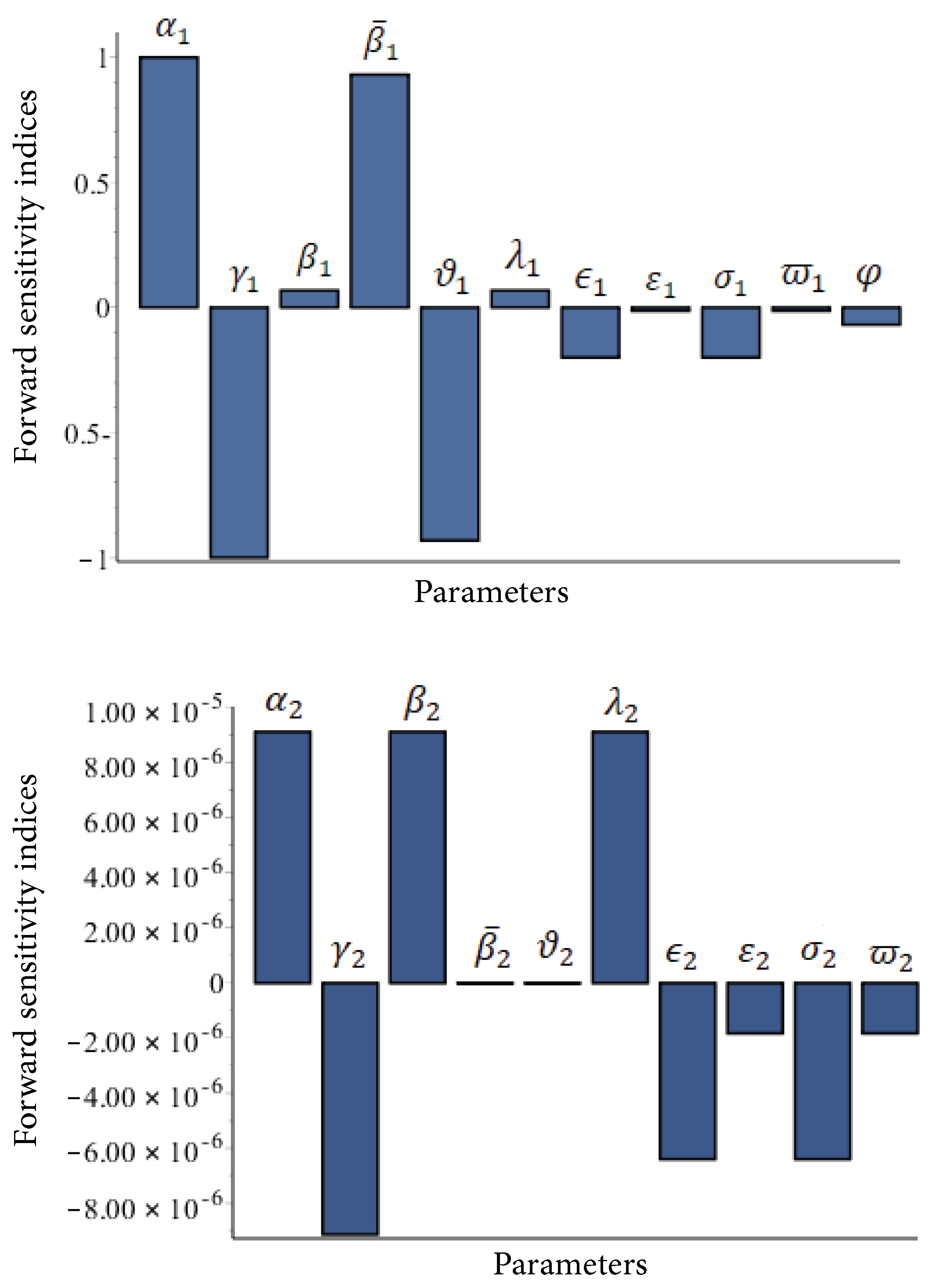
4.1. Sensitivity Analysis
4.2. Stability of the Equilibria
- -
- The chosen delay parameters are
- -
- I.1: ;
- I.2: ;
- I.3: , where
- Case : ;
- Case : ;
- Case : ;
- Case :
- (i)
- If , then , and the IFE is GAS;
- (ii)
- If , then , and will become unstable.
5. Conclusions
- (i)
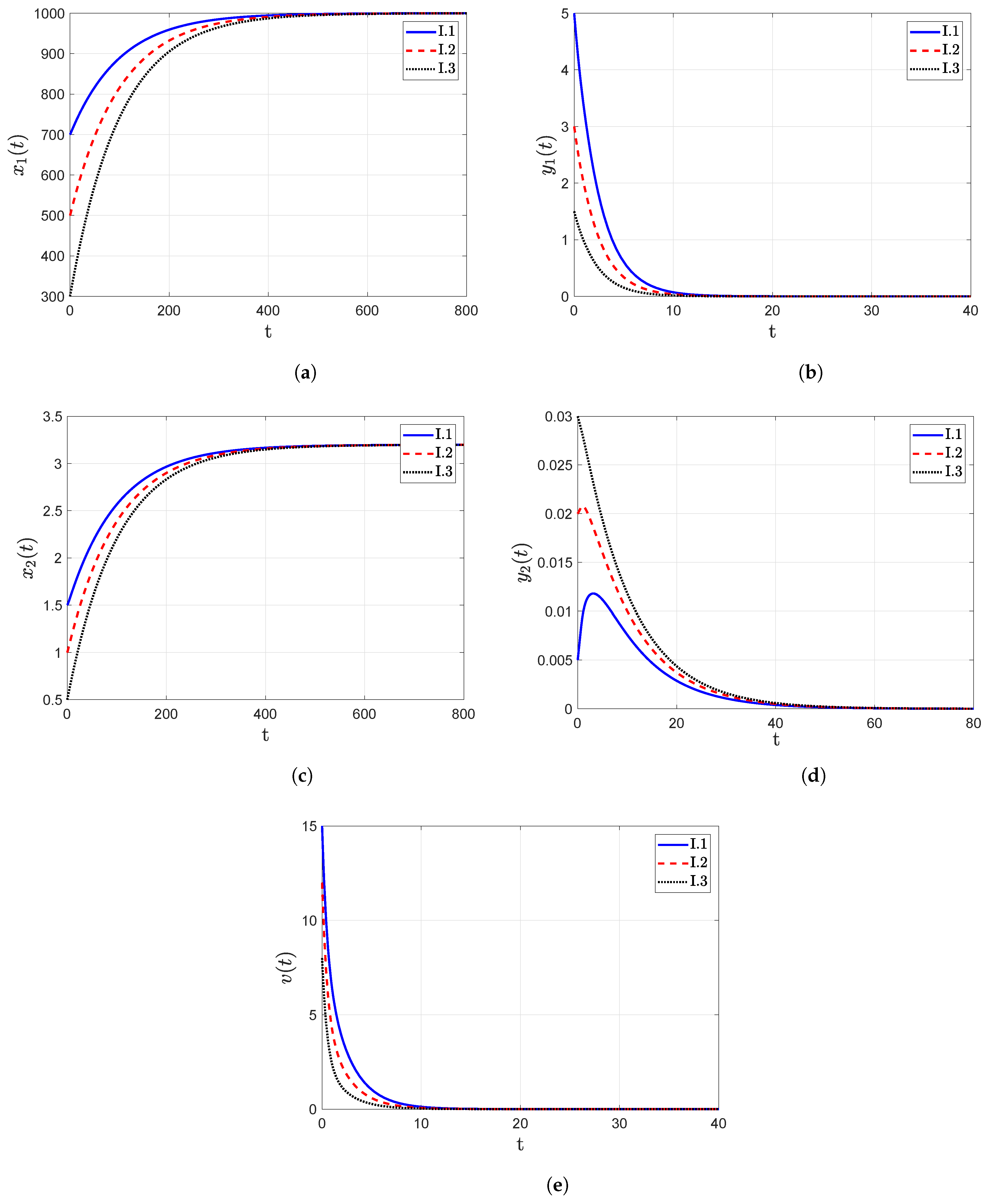
- The trajectory diagrams tend towards the IFE when the reproduction number , as shown in Figure 3. One significant finding from these figures is that for different initial conditions assumed for the model categories, their trajectories still point towards the IFE over the passage of time. These findings also confirm the global asymptotic stability analysis results, which were presented in Section 3.3.
- (ii)
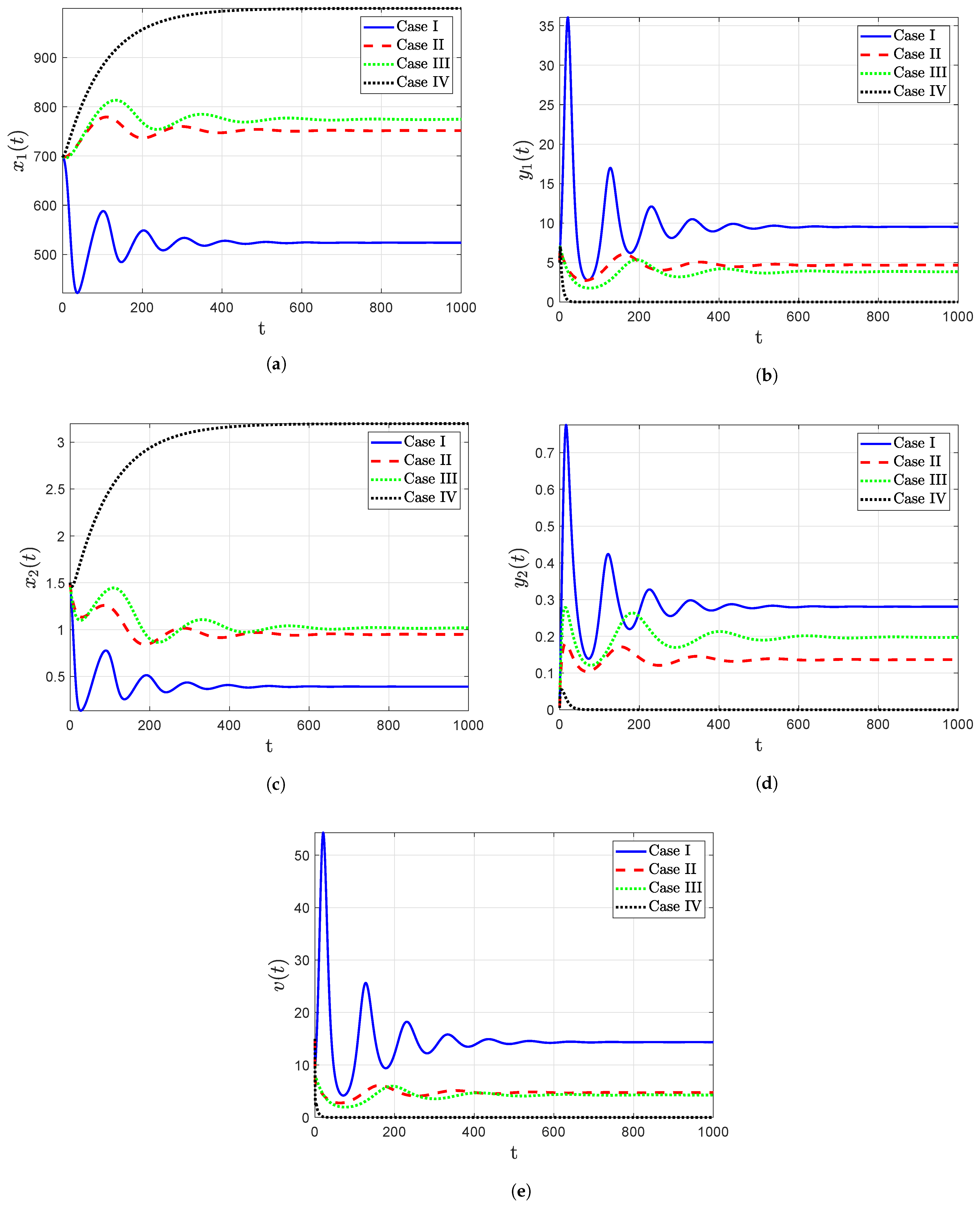
- The trajectory diagrams tend towards the IPE for different initial conditions when the reproduction number , as shown in Figure 4, which confirms that the point IPE is GAS when . Consequently, the model leads to an outcome in which the person is infected with HIV-1.
- (iii)
- From Figure 5 and Table 5, increasing the time delay causes a decrease in the reproduction number, resulting in an increase in uninfected CD T cells, resulting in a decrease in viral load. That is, time delay contributes a very significant effect in governing the dynamic behavior of the system and should not be neglected in HIV-1 modeling.
Author Contributions
Funding
Data Availability Statement
Acknowledgments
Conflicts of Interest
References
- UNAIDS. Global HIV & AIDS Statistics Fact Sheet; UNAIDS: Geneva, Switzerland, 2022; Available online: http://www.unaids.org/en/resources/fact-sheet (accessed on 20 August 2022).
- Avendano, R.; Esteva, L.; Flores, J.A.; Allen, J.F.; Gómez, G.; López-Estrada, J. A Mathematical Model for the Dynamics of Hepatitis C. J. Theor. Med. 2002, 4, 2253–2263. [Google Scholar] [CrossRef] [Green Version]
- Elaiw, A.M.; Alsulami, R.S.; Hobiny, A.D. Hobiny, Modeling and stability analysis of within-host IAV/SARS-CoV-2 coinfection with antibody immunity. Mathematics 2022, 10, 4382. [Google Scholar] [CrossRef]
- Nath, B.J.; Dehingia, K.; Mishra, V.N.; Chu, Y.M.; Sarmah, H.K. Mathematical analysis of a within-host model of SARS-CoV-2. Adv. Differ. Equ. 2021, 2021, 113. [Google Scholar] [CrossRef]
- Azoz, S.A.; Hussien, F. Mathematical study of a fractional-order general pathogen dynamic model with immune impairment. In Towards Intelligent Systems Modeling and Simulation; Springer: Cham, Switzerland, 2022; pp. 379–398. [Google Scholar]
- Elaiw, A.M.; Al Agha, A.D.; Azoz, S.A.; Ramadan, E. Global analysis of within-host SARS-CoV-2/HIV coinfection model with latency. Eur. Phys. J. Plus 2022, 137, 174. [Google Scholar] [CrossRef]
- Ghosh, I.; Tiwari, P.K.; Samanta, S.; Elmojtaba, I.M.; Al-Salti, N.; Chattopadhyay, J. A simple SI-type model for HIV/AIDS with media and self-imposed psychological fear. Math. Biosci. 2018, 306, 160–169. [Google Scholar] [CrossRef]
- Majumder, M.; Tiwari, P.K.; Pal, S. Impact of saturated treatments on HIV-TB dual epidemic as a consequence of COVID-19: Optimal control with awareness and treatment. Nonlinear Dyn. 2022, 109, 143–176. [Google Scholar] [CrossRef]
- Medda, R.; Tiwari, P.K.; Pal, S. Chaos in a nonautonomous model for the impact of media on disease outbreak. Int. J. Model. Simul. Sci. Comput. 2022, 2350020. [Google Scholar] [CrossRef]
- Majumder, M.; Tiwari, P.K.; Pal, S. Impact of nonlinear infection rate on HIV/AIDS considering prevalence-dependent awareness. Math. Methods Appl. Sci. 2023, 46, 3821–3848. [Google Scholar] [CrossRef]
- Perelson, A.S.; Essunger, P.; Cao, Y.; Vesanen, M.; Hurley, A.; Saksela, K.; Markowitz, M.; Ho, D.D. Decay characteristics of HIV-1-infected compartments during combination therapy. Nature 1997, 387, 188–191. [Google Scholar] [CrossRef]
- Culshaw, R.V.; Ruan, S. A delay-differential equation model of HIV infection of CD4+ T-cells. Math. Biosci. 2000, 165, 27–39. [Google Scholar] [CrossRef]
- Li, Y.; Xu, R.; Mao, S. Global dynamics of a delayed HIV-1 infection model with CTL immune response. Discret. Dyn. Nat. Soc. 2011, 2011, 673843. [Google Scholar] [CrossRef] [Green Version]
- AlAgha, A.D.; Elaiw, A.M. Stability of a general reaction-diffusion HIV-1 dynamics model with humoral immunity. Eur. Phys. J. Plus 2019, 134, 390. [Google Scholar] [CrossRef]
- Hethcote, H. The mathematics of infectious diseases. Siam Rev. 2000, 42, 599–653. [Google Scholar] [CrossRef] [Green Version]
- Attaullah; Sohaib, M. Mathematical modeling and numerical simulation of HIV infection model. Results Appl. Math. 2020, 7, 100–118. [Google Scholar] [CrossRef]
- Wang, Y.; Qi, K.; Jiang, D. An HIV latent infection model with cell-to-cell transmission and stochastic perturbation. Chaos Solitons Fractals 2021, 151, 111215. [Google Scholar] [CrossRef]
- Culshaw, R.V.; Ruan, S.; Webb, G. A mathematical model of cell-to-cell spread of HIV-1 that includes a time delay. J. Math. Biol. 2003, 46, 425–444. [Google Scholar] [CrossRef]
- Yang, Y.; Zou, L.; Ruan, S. Global dynamics of a delayed within-host viral infection model with both virus-to-cell and cell-to-cell transmissions. Math. Biosci. 2015, 270, 183–191. [Google Scholar] [CrossRef]
- Ełaiw, A.M.; Raezah, A.A.; Hattaf, K. Stability of HIV-1 infection with saturated virus-target and infected-target incidences and CTL immune response. Int. J. Biomath. 2017, 5, 1750070. [Google Scholar] [CrossRef]
- Alofi, B.S.; Azoz, S.A. Stability of general pathogen dynamic models with two types of infectious transmission with immune impairment. AIMS Math. 2021, 6, 114–140. [Google Scholar] [CrossRef]
- Nowak, M.A.; Bangham, C.R.M. Population dynamics of immune responses to persistent viruses. Science 1996, 272, 74–79. [Google Scholar] [CrossRef] [Green Version]
- Mittler, J.E.; Sulzer, B.; Neumann, A.U.; Perelson, A.S. Influence of delayed viral production on viral dynamics in HIV-1 infected patients. Math. Biosci. 1998, 152, 143–163. [Google Scholar] [CrossRef]
- Nelson, P.W.; Murray, J.D.; Perelson, A.S. A model of HIV-1 pathogenesis that includes an intracellular delay. Math. Biosci. 2000, 163, 201–215. [Google Scholar] [CrossRef]
- Nelson, P.W.; Perelson, A.S. Mathematical analysis of delay differential equation models of HIV-1 infection. Math. Biosci. 2002, 179, 73–94. [Google Scholar] [CrossRef]
- Dixit, N.M.; Perelson, A.S. Complex patterns of viral load decay under antiretroviral therapy: Influence of pharmacokinetics and intracellular delay. J. Theor. Biol. 2004, 226, 95–109. [Google Scholar] [CrossRef]
- Perelson, A.S.; Nelson, P.W. Mathematical analysis of HIV-1 dynamics in vivo. SIAM Rev. 1999, 41, 3–44. [Google Scholar] [CrossRef] [Green Version]
- Callaway, D.S.; Perelson, A.S. HIV-1 infection and low steady state viral loads. Bull. Math. Biol. 2002, 64, 29–64. [Google Scholar] [CrossRef]
- Elaiw, A.M. Global properties of a class of HIV models. Nonlinear Anal. Real World Appl. 2010, 11, 2253–2263. [Google Scholar] [CrossRef]
- Wang, X.; Elaiw, A.M.; Song, X. Global properties of a delayed HIV infection model with CTL immune response. Appl. Math. Comput. 2012, 218, 9405–9414. [Google Scholar] [CrossRef]
- Elaiw, A.M.; Elnahary, E.K. Analysis of general humoral immunity HIV dynamics model with HAART and distributed delays. Mathematics 2019, 7, 157. [Google Scholar] [CrossRef] [Green Version]
- Elaiw, A.M.; Raezah, A.A.; Azoz, S.A. Stability of delayed HIV dynamics models with two latent reservoirs and immune impairment. Adv. Differ. Equ. 2018, 50, 414. [Google Scholar] [CrossRef]
- Adams, B.M.; Banks, H.T.; Kwon, H.-D.; Tran, H.T. Dynamic multidrug therapies for HIV: Optimal and STI control approaches. Math. Biosci. Eng. 2004, 1, 223–241. [Google Scholar] [CrossRef]
- Adams, B.M.; Banks, H.T.; Davidian, M.; Kwon, H.D.; Tran, H.T.; Wynne, S.N.; Rosenberg, E.S. Rosenberg HIV dynamics: Modeling, data analysis, and optimal treatment protocols. J. Comput. Appl. Math. 2005, 184, 10–49. [Google Scholar] [CrossRef] [Green Version]
- Elaiw, A.M.; Xia, X. HIV dynamics: Analysis and robust multirate MPC-based treatment schedules. J. Math. Anal. Appl. 2009, 356, 285–301. [Google Scholar] [CrossRef] [Green Version]
- Van den Driessche, P.; Watmough, J. Reproduction numbers and sub-threshold endemic equilibria for compartmental models of disease transmission. Math. Biosci. 2002, 180, 29–48. [Google Scholar] [CrossRef]
- Khalil, H.K. Nonlinear Systems, 3rd ed.; Prentice Hall: Upper Saddle River, NJ, USA, 2002. [Google Scholar]
- Pukdeboon, C. A review of fundamentals of Lyapunov theory. J. Appl. Sci. 2011, 10, 55–61. [Google Scholar]
- Li, Y.; Zhang, J.; Qiong, W. Adaptive Sliding Mode Neural Network Control for Nonlinear Systems; Academic Press: London, UK, 2018. [Google Scholar]
- LaSalle, J.P. The Stability of Dynamical Systems; SIAM: Philadelphia, PA, USA, 1976. [Google Scholar]
- Barbashin, E.A. Introduction to the Theory of Stability; Wolters-Noordhoff: Groningen, The Netherlands, 1970. [Google Scholar]
- Lyapunov, A.M. The General Problem of the Stability of Motion. Int. J. Control 1992, 55, 531–534. [Google Scholar] [CrossRef]
- Hale, J.K.; Lunel, S.M.V. Introduction to Functional Differential Equations, 1st ed.; Springer Science & Business Media, LLC: New York, NY, USA, 1993. [Google Scholar]
- Perelson, A.S.; Kirschner, D.E.; De Boer, R. Dynamics of HIV infection of CD4+T cells. Math. Biosci. 1993, 114, 81–125. [Google Scholar] [CrossRef] [Green Version]
- Li, F.; Ma, W. Dynamics analysis of an HTLV-1 infection model with mitotic division of actively infected cells and delayed CTL immune response. Math. Methods Appl. Sci. 2018, 41, 3000–3017. [Google Scholar] [CrossRef]
- Elaiw, A.M.; AlShamrani, N.H. HTLV/HIV dual Infection: Modeling and analysis. Mathematics 2021, 9, 51. [Google Scholar] [CrossRef]
- AlShamrani, N.H. Stability of an HTLV-HIV coinfection model with multiple delays and CTL-mediated immunity. Adv. Differ. Equ. 2021, 2, 1–57. [Google Scholar] [CrossRef]
- Mohri, H.; Bonhoeffer, S.; Monard, S.; Perelson, A.S.; Ho, D.D. Rapid turnover of T lymphocytes in SIV-infected rhesus macaques. Science 1998, 279, 1223–1227. [Google Scholar] [CrossRef]
- Perelson, A.S.; Neumann, A.U.; Markowitz, M.; Leonard, J.M.; Ho, D.D. HIV-1 dynamics in vivo: Virion clearance rate, infected cell life-span, and viral generation time. Science 1996, 271, 1582–1586. [Google Scholar] [CrossRef] [Green Version]
- Zarin, R.; Khan, A.; Raezah, A.A. Computational modeling of fractional COVID-19 model by Haar wavelet collocation Methods with real data. Math. Biosci. Eng. 2023, 20, 11281–11312. [Google Scholar] [CrossRef]
- Fan, X.; Brauner, C.-M.; Wittkop, L. Mathematical analysis of a HIV model with quadratic logistic growth term. Discret. Contin. Dyn. Syst. Ser. B 2012, 17, 2359–2385. [Google Scholar] [CrossRef]
- Elaiw, A.M.; Alsaedi, A.J.; Al Agha, A.D.; Hobiny, A.D. Global stability of a humoral immunity COVID-19 model with logistic growth and delays. Mathematics 2022, 10, 1857. [Google Scholar] [CrossRef]
- Wang, L.; Li, M.Y. Mathematical analysis of the global dynamics of a model for HIV infection of CD4+T cells. Math. Biosci. 2006, 200, 44–57. [Google Scholar] [CrossRef]


| Case | Conditions | ||
|---|---|---|---|
| 1 | |||
| 2 | |||
| 3 | (from Lemma 2) | ||
| 4 | − | ||
| 5 | − | ||
| 6 | − |
| Case | Conditions | ||
|---|---|---|---|
| 1 | |||
| 2 | |||
| 3 | (from Lemma 6) | ||
| 4 | − | ||
| 5 | − | ||
| 6 | − |
| Parameter | Value | References | Parameter | Value | References | Parameter | Value | Source |
|---|---|---|---|---|---|---|---|---|
| 10 | [44,45,46] | [31] | [47] | |||||
| [28,46,48] | [33,34] | 1 | Assumed | |||||
| [24,27,49] | [27] | 1 | [32] | |||||
| 6 | [32] | 6 | [32] | 1 | [32] | |||
| 2 | [46] |
| Parameter | Sensitivity Index | Parameter | Sensitivity Index | Parameter | Sensitivity Index |
|---|---|---|---|---|---|
Disclaimer/Publisher’s Note: The statements, opinions and data contained in all publications are solely those of the individual author(s) and contributor(s) and not of MDPI and/or the editor(s). MDPI and/or the editor(s) disclaim responsibility for any injury to people or property resulting from any ideas, methods, instructions or products referred to in the content. |
© 2023 by the authors. Licensee MDPI, Basel, Switzerland. This article is an open access article distributed under the terms and conditions of the Creative Commons Attribution (CC BY) license (https://creativecommons.org/licenses/by/4.0/).
Share and Cite
Raezah, A.A.; Dahy, E.; Elnahary, E.K.; Azoz, S.A. Stability of HIV-1 Dynamics Models with Viral and Cellular Infections in the Presence of Macrophages. Axioms 2023, 12, 617. https://doi.org/10.3390/axioms12070617
Raezah AA, Dahy E, Elnahary EK, Azoz SA. Stability of HIV-1 Dynamics Models with Viral and Cellular Infections in the Presence of Macrophages. Axioms. 2023; 12(7):617. https://doi.org/10.3390/axioms12070617
Chicago/Turabian StyleRaezah, Aeshah A., Elsayed Dahy, E. Kh. Elnahary, and Shaimaa A. Azoz. 2023. "Stability of HIV-1 Dynamics Models with Viral and Cellular Infections in the Presence of Macrophages" Axioms 12, no. 7: 617. https://doi.org/10.3390/axioms12070617