Article

The Dynamics of a General Model of the Nonlinear Difference Equation and Its Applications

by
Osama Moaaz
1,2,* and
Aseel A. Altuwaijri
1
1
Department of Mathematics, College of Science, Qassim University, P.O. Box 6644, Buraydah 51452, Saudi Arabia
2
Department of Mathematics, Faculty of Science, Mansoura University, Mansoura 35516, Egypt
*
Author to whom correspondence should be addressed.
Axioms 2023, 12(6), 598; https://doi.org/10.3390/axioms12060598
Submission received: 9 May 2023 / Revised: 8 June 2023 / Accepted: 13 June 2023 / Published: 16 June 2023
(This article belongs to the Special Issue Advances in Difference Equations)

Abstract

:
This article investigates the qualitative properties of solutions to a general difference equation. Studying the properties of solutions to general difference equations greatly contributes to the development of theoretical methods and provides many pieces of information that may help to understand the behavior of solutions of some special models. We present the sufficient and necessary conditions for the existence of prime period-two and -three solutions. We also obtain a complete perception of the local stability of the studied equation. Then, we investigate the boundedness and global stability of the solutions. Finally, we support the validity of the results by applying them to some special cases, as well as numerically simulating the solutions.

1. Introduction

In both pure and applied mathematics, meteorology, physics, population dynamics, and engineering, there are many applications for the study of functional differential equations (FDEs) and difference equations (DIEs). The properties of these equations of different sorts are a topic that is addressed by all of these fields. For global existence and uniqueness theorems for differential equations, see books [1], and for the fundamentals of DIEs, see books [2,3,4,5]. Pure mathematics is concerned with the existence and uniqueness of solutions. The rigorous justification of the qualitative properties of solutions, such as oscillation, periodicity, stability (local and global), Hopf bifurcation, control, etc., is emphasized in applied mathematics [4,6,7,8].
DIEs are used to describe how a phenomena evolves in the real world when most observations of a temporally changing variable are discrete. These equations consequently become essential in mathematical models. Applications heavily rely on nonlinear DIEs of an order larger than one. Additionally, these equations naturally occur as discrete analogs and numerical answers to differential and delay differential equations that model a variety of diverse phenomena in different sciences; see [5,9,10,11,12,13,14,15].
Investigation of the qualitative properties of the DIE
u n + 1 = u n 1 P u n , u n 1
is the focus of this paper, where P t , s : 0 , 2 0 , is continuous and homogenous with degree α , where α is a non-negative real number. Furthermore, the initial conditions u 1 , u 0 are nonnegative real numbers.
The study of the qualitative properties of solutions of DIEs was and still is a vital and active research field. As a result of the rapid development of science and technology, many biological, technological, geological and other issues have arisen. Many mathematical models have emerged with these issues. Studying the qualitative behavior of the general DIEs may significantly contribute to eliciting the characteristics of the solutions of these new models.
In this work, we are interested in investigating some qualitative properties of solutions to the general DIE (1). We begin by deducing the sufficient and necessary conditions for the existence of prime period-two solutions of DIE (1). Then, we investigate the local asymptotic stability of a two-cycle solution of DIE (1). Moreover, we obtain criteria that guarantee the existence of prime period-three solutions, and apply the results in this section to some special cases to support the theoretical results. We also study the local and global stability of solutions to DIE (1). We present several lemmas and theorems that set sufficient criteria for the convergence of solutions to the equilibrium point. Finally, through examples and numerical simulations, we present some theoretical results for some special cases of the studied equation and simulate the results numerically through the MATHEMATICA program.
In order to verify the periodicity of solutions, the methodology of this study is based on the use of an improved technique discussed in [16,17]. Using some theorems in [18], we investigate the local and global stability of the equilibrium points of the studied equation.
In the following, we review some of the previous results in the literature, which contributed significantly to the development of the study of the qualitative properties of solutions of DIEs.
The Riccati DIEs model
u n + 1 = a 1 + a 2 u n a 3 + a 4 u n ,
is one of the most intriguing ones, where a i R , for i = 1 , 2 , 3 , 4 , see [12]. A special application of DIE (2) offers the traditional Beverton–Holt model on the dynamics of exploited fish populations [10]. In [19], Kuruklis et al. examined some properties of solutions of the Pielou’s discrete logistic model [20]
u n + 1 = a u n 1 + u n 1 ,
where a 1 . May [21] offered the DIE
u n + 1 = u n exp c 1 2 u n 1 u n + u n exp c 1 2 u n ,
where c > 0 , as an illustration of a map produced by a straightforward model for frequency-dependent natural selection. The model of the expansion of the flour beetle population
u n + 1 = a 1 u n + a 2 u n 2 exp a 3 u n a 4 u n 2 ,
was proven to be globally stable by Kuang et al. [22], where a 1 0 , 1 ,   a 2 , a 3 , a 4 0 , , a 2 0 and a 3 + a 4 > 0 .
Many researchers have been interested in studying general models of DIEs. In [23], Stevic studied the periodic nature of the general DIE
u n + 1 = F u n , u n 1 a + u n ,
where a , u 1 , u 0 R + and F C R + × R + , R + and
F k , l F l , m = k m G k , l , m a k l ,
for some G C R + × R + , R + , such that
1 k G k , l , m 0 as k , l , m and sup 1 a + k G k , l , m < .
Karakostas and Stevic [24] studied the qualitative properties of solutions to the general DIE
u n + 1 = a + u n r F u n , u n 1 , , u n r + 1
where a 0 . In [25], the global stability of solutions to the general DIE
u n + = F u n k , u n l ,
has been studied, where k , l N , k < l . Moaaz et al. [26] discussed the qualitative properties of solutions to the DIE
u n + 1 = f u n l , u n k
where k , l N , and f is a homogenous function with degree z e r o .
Recently, Elsayed et al. [27,28,29], Al-Basyouni and Elsayed [30], and Kara and Yazlik [31] established solutions to for certain categories of DIEs. In [27], Elsayed and Alofi studied the properties of solutions to a system of DIEs and provided solutions to this system. Elsayed et al. [28] considered the DIE
u n + 1 = a u n 1 + b u n 1 u n 4 c u n 4 + k u n 2 ,
and provided solutions to this DIE. The periodic properties and construction of the solution for some rational system of DIEs were presented in [29,30]. Moreover, for fractional difference equations and systems, there are many interesting results in [32,33].

2. Definitions and Preliminary Results

The fundamental definitions, including equilibrium points, local and global stability, boundedness, and periodicity, are presented in this section. We also review some basic theorems.
Consider a DIE in the form
u n + 1 = ψ u n l , u n k , n = 0 , 1 , ,
where ψ C I × I , I , l , k Z + 0 ,  I is some interval of R , and m = max l , k .
Definition 1.
If a point u e is a fixed point of ψ, then it is said to be an equilibrium point (EQP) of DIE (6).
Definition 2.
Assume that u e is an EQP of (6).
S1. 
If for all ϵ > 0 there is a δ > 0 such that u n u e < ϵ for all n m , for u j I , j = 0 , 1 , , m with j = 0 m u j u e < δ , then u e is said to be locally stable.
S2. 
If u e is locally stable and there is γ > 0 such that lim n u n = u e for u j I , j = 0 , 1 , , m with j = 0 m u j u e < δ , then u e is said to be locally asymptotically stable.
S3. 
If lim n u n = u e for all u j I , j = 0 , 1 , , m , then u e is said to be a global attractor.
S4. 
If u e is locally stable and a global attractor, then it is said to be globally asymptotically stable.
S5. 
If u e is not locally stable, then it is said to be unstable.
Definition 3.
A sequence u n n = m is called a periodic solution with period ℓ if u n + = u n for all n m .
Definition 4.
A sequence u n n = m is called a periodic solution with prime period ℓ if = min s Z + : u n + s = u n f o r a l l n m .
Definition 5.
The linearized equation of (6) about the EQP u e is defined by Z n + 1 = i = 0 m λ i Z n i where
λ i = ψ u e , u e u n i .
Theorem 1
([18], Theorem 1.4.6). Suppose that ψ C I 2 , I , where I R , and ψ t , s satisfies the following properties:
(a) 
ψ t 0  and  ψ s 0 , for all  t , s I 2 ,
(b) 
The DIE
u n + 1 = ψ u n , u n 1
has no solutions of prime period two in  I .
Then, DIE (7) has a unique EQP  u e  and all solutions of (7) converge to  u e .
Theorem 2
([18], Theorem 1.4.5). Suppose that ψ C I 2 , I ,  where  I R , and  ψ t , s satisfies the following properties:
(a) 
ψ t 0  and  ψ s 0 for all  t , s I 2 ,
(b) 
If  ( s , B ) I 2  is a solution of the system
ψ s , B = s , ψ B , s = B ,
then  s = B .
Then, DIE (7) has a unique EQP  u e  and all solutions of (7) converge to  u e .

3. Dynamics of Equation (1)

In the following, we study the behavior of solutions to DIE (1). Through the next results, we need to define the following functions:
P 1 t , s = t P t , s
and
P 2 t , s = s P t , s .

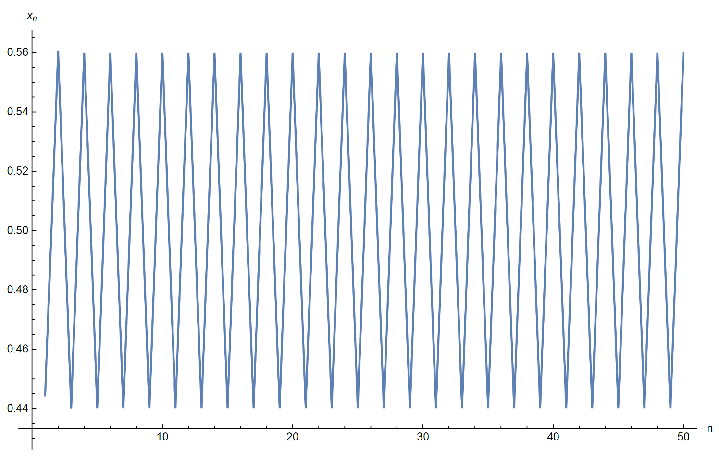
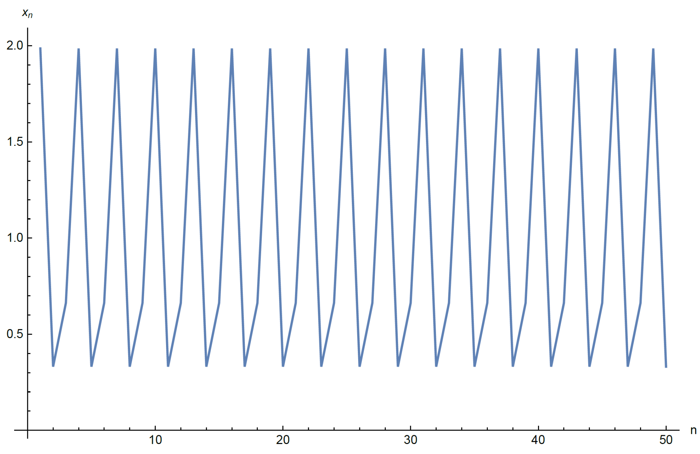
3.1. Periodic Behavior of Solutions

In the following, we provide the necessary and sufficient conditions for the existence of prime period-two and -three solutions to DIE (1).

3.1.1. Existence of Prime Period-Two Solutions

Theorem 3.
Suppose that α > 0 . The necessary and sufficient condition for the existence of periodic solutions with period-two of DIE (1) is the existence of a constant l R + / 1 that satisfies P l , 1 = P 1 , l .
Proof. 
Suppose that DIE (1) has the solution of the form , σ , ϱ , σ , ϱ , . Then, we can obtain
σ = σ P ϱ , σ ; ϱ = ϱ P σ , ϱ .
Therefore,
ϱ α P 1 , σ ϱ = 1 ,
and
ϱ α P σ ϱ , 1 = 1 .
Hence, there is a l = σ / ϱ such that P l , 1 = P 1 , l .
On the other hand, we suppose that P l , 1 = P 1 , l . Now, we choose u 1 = l P 1 / α 1 , l and u 0 = P 1 / α 1 , l , where l R + / 1 . Thus,
u 1 = u 1 P u 0 , u 1 = l P 1 / α 1 , l P P 1 / α 1 , l , l P 1 / α 1 , l = l P 1 / α 1 , l P 1 1 , l P 1 , l = l P 1 / α 1 , l = u 1 .
Also,
u 2 = u 0 P u 1 , u 0 = P 1 / α 1 , l P 1 1 , l P l , 1 = P 1 / α 1 , l = u 0 .
Similarly, we have u 2 r = u 0 and u 2 r + 1 = u 1 for all r = 1 , 2 , .
Then, the proof is complete. □
Theorem 4.
Suppose that α = 0 . The necessary and sufficient condition for the existence of periodic solutions with period-two of DIE (1) is the existence of a constant l R + / 1 that satisfies P l , 1 = 1 = P 1 , l .
Proof. 
Proceeding as in the proof of Theorem 1, we can prove that the condition is necessary.
On the other hand, we suppose that P l , 1 = P 1 , l . Now, we choose u 1 = c and u 0 = c k , where l R + / 1 . Thus,
u 1 = c P c l , c = c P l , 1 = c
Also,
u 2 = c l P c , c l = c l P 1 , l = c l .
Similarly, we have u 2 r = c and u 2 r + 1 = c l for all r = 1 , 2 , .
Then, the proof is complete. □
Example 1.
Let the DIE
u n + 1 = u n 1 a u n + b u n 1 ,
where a , b R + . We note that P t , s = a t + b s is homogenous with degree o n e . Using Theorem 3, the necessary and sufficient condition for the existence of periodic solutions with period-two of DIE (1) is the existence of a constant l R + / 1 that satisfies a l + b = a + b l , and so a b l 1 = 0 , i.e., a = b , see Figure 1.

3.1.2. Local Asymptotic Stability of a Two Cycle

Suppose that DIE (1) has a solution with two cycle , σ , ϱ , σ , ϱ , . Now, we set
t n = u n 1 and s n = u n .
Then, DIE (1) is equivalent to the system
t n + 1 = s n , s n + 1 = t n P s n , t n .
Next, we define F : 0 , 2 0 , 2 by
F t s = s t P s , t .
Therefore, we have that
σ ϱ
is a fixed point of F 2 : = F F , where
F 2 t s = t P s , t s P t P s , t , s
The Jacobian matrix J F 2 at σ , ϱ takes the form
J F 2 σ ϱ = A B C D ,
where
A : = P ϱ , σ σ P 2 ϱ , σ P 2 ϱ , σ , B : = σ P 1 ϱ , σ P 2 ϱ , σ , C : = A ϱ P 2 σ P ϱ , σ , ϱ P 1 σ P ϱ , σ , ϱ ,
and
D : = 1 P 2 σ P ϱ , σ , ϱ P σ P ϱ , σ , ϱ ϱ B P 1 σ P ϱ , σ , ϱ + P 2 σ P ϱ , σ , ϱ .
In the event that the eigenvalues of J F 2 at σ , ϱ are inside the unit disk, the two-cycle solution is locally asymptotically stable. Using Theorem 1.1.1 (c) in [18], the eigenvalues of J F 2 at σ , ϱ are inside the unit disk if
K < 1 + L and L < 1 ,
where
K = A + D
and
L = A D B C .
Example 2.
Consider the DIE (8) where a , b R + . From Theorem 3, for l R + / 1 , there is a prime period two solution
, l a 1 + l , 1 a 1 + l , l a 1 + l , 1 a 1 + l , .
It is easy to verify that
A = 1 1 + l , B = l 1 + l , C = l 1 + l ,
and
D = l 2 + l 1 + l 2 .
The two cycle solution (9) of DIE (8) is locally asymptotically stable if l 1 + l < 1 .

3.1.3. Existence of Prime Period-Three Solutions

Theorem 5.
Assume that α > 0 . Then, DIE (1) has a prime period-three solution if and only if the system
P l , 1 = k 2 α l P k , 1 , P 1 / k l , 1 = l 1 α k P l , 1 , P k , 1 = k 2 1 l 2 2 P 1 / k l , 1 ,
has a solution k , l , where k , l R + , and at least one of k , l is not equal to one.
Proof. 
Suppose that DIE (1) has the solution , δ , β , γ , δ , β , γ , . Then, we can obtain
γ = δ P β , δ , δ = β P γ , β , β = γ P δ , γ .
Set β / δ = k and γ / β = l , we arrive at
γ = δ 1 α P k , 1 , δ = β 1 α P l , 1 , β = γ 1 α P 1 / k l , 1 .
Thus, we obtain
P l , 1 = k 2 α l P k , 1 ,
and
P 1 / k l , 1 = l 1 α k P l , 1 .
Then, system (10) has the solution β / δ , γ / β .
On the other hand, we suppose that system (10) has a solution k , l , where k , l R + , and at least one of k , l is not equal to one. Now, we choose
u 1 = 1 k l P k , 1 1 / α , u 0 = k P l , 1 1 / α .
Thus, by using (10), we have
u 1 = u 1 P u 0 , u 1 = 1 k 1 / α l 1 / α P 1 / α k , 1 1 P k 1 / α P 1 / α l , 1 , 1 k 1 / α l 1 / α P 1 / α k , 1 = k l k 1 / α l 1 / α P 1 / α k , 1 = k l k 1 / α l 1 / α 1 k 1 α α l 2 α α P 1 / α 1 / k l , 1 = l P 1 / k l , 1 1 / α .
Additionally,
u 2 = u 0 P u 1 , u 0 = k 1 / α P 1 / α l , 1 1 P l 1 / α P 1 / α 1 / k l , 1 , k 1 / α P 1 / α l , 1 = k 1 / α P 1 / α l , 1 1 k = k 1 / α k 2 α α l 1 / α 1 k 1 P 1 / α k , 1 = 1 k l P k , 1 1 / α = u 1
Similarly, we can prove that u 3 = u 0 . Proceeding with the same approach, we conclude that
u 3 r 1 = u 1 , u 3 r = u 0 , and u 3 r + 1 = u 1 , for all r = 1 , 2 , .
Therefore, the proof is complete. □
Theorem 6.
Suppose that α = 0 . DIE (1) has a prime period-three solution if and only if the system
0 = 1 k l P k , 1 , 0 = k P l , 1 , 0 = l P 1 / k l , 1
has a solution k , l , m , where k , l , m R + , and at least one of k , l , m is not equal to one.
Proof. 
Suppose that DIE (1) has the solution , δ , β , γ , δ , β , γ , . As in the proof of Theorem 5, we arrive at
γ = δ P k , 1 , δ = β P l , 1 , β = γ P 1 / k l , 1 .
Thus, we obtain
k l P k , 1 = 1
k = P l , 1
and
l = P 1 / k l , 1 .
Then, system (10) has the solution β / δ , γ / β .
On the other hand, we assume that (10) has a solution k , l , where k , l R + , and at least one of k , l is not equal to one. Now, we choose u 1 = c and u 0 = c k , where k R + and c is an arbitrary positive real number. Therefore,
u 1 = c P c k , c = c P k , 1 = c k l , u 2 = c k P c k l , c k = c k P l , 1 = c = u 1 ,
and
u 3 = u 1 P u 2 , u 1 = c k l P c , c k l = c k l P 1 / k l , 1 = c k = u 0 .
Proceeding with the same approach, we conclude that
u 3 r 1 = u 1 , u 3 r = u 0 ,   and u 3 r + 1 = c k l , for all r = 1 , 2 , .
Therefore, the proof is complete. □
Example 3.
Consider the DIE
u n + 1 = u n u n 1 2 a u n u n 1 + b u n 2 + c u n 1 2 ,
where a , b and c R / 0 . We note that
P t , s = a + b t s + c s t
is homogenous with degree z e r o . Using Theorem 5, DIE (12) has a prime period-three solution if the system
0 = 1 k l a + b k + c 1 k , 0 = k a + b l + c 1 l , 0 = l a + b 1 k l + c k l
has the solution.
Consider the special case when a = 2521 561 ,   b = 380 187 , and c = 223 187 . DIE (12) has a prime period-three solution , 1 , 2 , 6 , 1 , 2 , 6 , , see Figure 2.

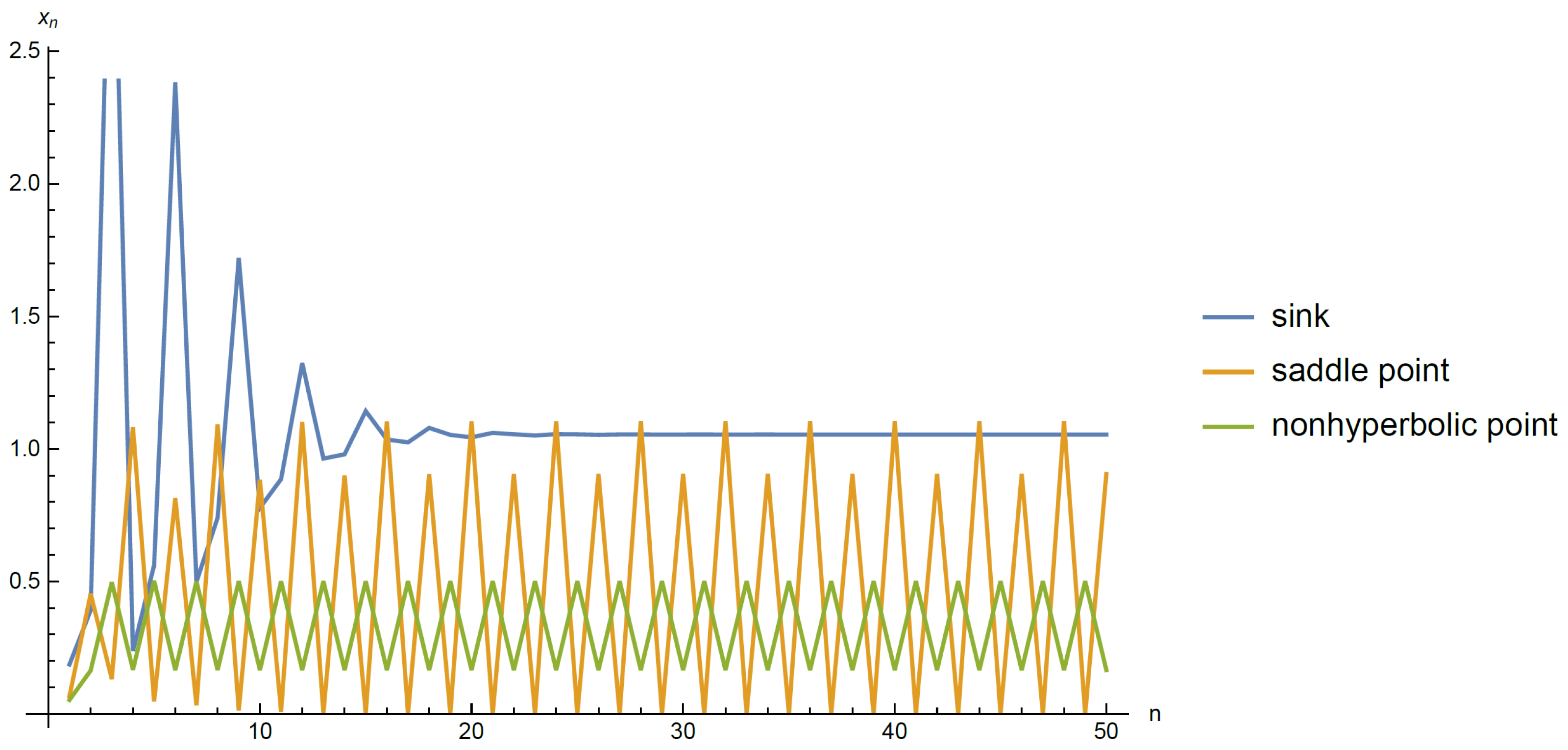
3.2. Stability Behavior of Solutions

Now, we define ϕ : 0 , 2 0 , by
ϕ t , s = s P t , s .
The EQP of DIE (1) is given by u e = ϕ u e , u e . Therefore,
1 P u e , u e 1 u e = 0 ,
this implies that the positive EQP
u e = 1 P 1 / α 1 , 1 , α > 0 .
The linearized equation of DIE (1) is
L n + 1 λ L n μ L n 1 = 0 ,
where
λ = ϕ u e , u e t = u e P 1 u e , u e P 2 u e , u e = P 1 1 , 1 u e α P 2 1 , 1
and
μ = ϕ u e , u e s = P u e , u e u e P 2 u e , u e P 2 u e , u e = P 1 , 1 P 2 1 , 1 u e α P 2 1 , 1 .
From (13), we obtain u e α = 1 / P 1 , 1 , and so
λ = P 1 1 , 1 P 1 , 1 and μ = 1 P 2 1 , 1 P 1 , 1 .
Remark 1.
Since P t , s is homogenous with degree α, we have P 1 t , s and P 2 t , s are homogenous with degree α 1 . Moreover, from Euler Theorem for homogeneous functions t P 1 t , s + s P 2 t , s = α P t , s . Thus, P 1 1 , 1 + P 2 1 , 1 = α P 1 , 1 .
Lemma 1.
The EQP u e of DIE (1) is locally asymptotically stable (sink) if
η < ρ < 2 κ ,
otherwise it is unstable. Furthermore, it has the following unstable cases:
(a) 
u e  is repeller if
κ ρ > κ a n d η < ρ ,
(b) 
u e  is a saddle point if
η 2 + 4 κ 2 > 4 κ ρ a n d η > ρ ,
(c) 
u e  is a nonhyperbolic point if
η = ρ ,
or
2 κ = ρ a n d η 2 κ ,
where κ = P 1 , 1 , η = P 1 1 , 1 , and ρ = P 2 1 , 1 .
Proof. 
The proof results directly from Theorem 1.1.1 in [18], so it was deleted. □
Lemma 2.
Assume that P 1 t , s 0 , P 2 t , s 0 , and
P l , 1 = P 1 , l l = 1 .
Then, all solutions of DIE (1) converge to u e .
Proof. 
From the definition of the function ϕ , it is easy to conclude that
ϕ t , s t = s P 1 t , s P 2 t , s 0 , ϕ t , s s = P t , s s P 2 t , s P 2 t , s 0 .
Since P l , 1 P 1 , l for all l R + / 1 , we obtain from Theorem 3 that DIE (1) has no solutions of prime period two. Therefore, from Theorem 1, all solutions of DIE (1) converge to u e . Hence, the proof is complete. □
Lemma 3.
Assume that α 1 , P 1 t , s 0 , and (16) holds. Then, all solutions of DIE (1) converge to u e .
Proof. 
From Remark 1, we have α P t , s s P 2 t , s 0 , which with the fact that α 1 gives P t , s s P 2 t , s . The rest of the proof is exactly as the proof of Theorem 2. □
Lemma 4.
Assume that α 1 , P 1 t , s 0 , and
P 1 , l = l 2 P l , 1 l = 1 .
Then, all solutions of DIE (1) converge to u e .
Proof. 
From Remark 1 and the fact that α 1 , we get P t , s α P t , s s P 2 t , s . From the definition of the function ϕ , it is easy to conclude that ϕ / t 0 and ϕ / s 0 .
Now, we suppose that s , B is a solution of the system
ϕ s , B = s , ϕ B , s = B .
Thus, we obtain
B = s P s , B and s = B P B , s .
Hence, we conclude that
B = s s α P 1 , B s and s = B s α P B s , 1 .
Set B / s = l , we arrive at
P 1 , l = l 2 P l , 1 .
Using (17), we obtain that l = 1 , and so B = s . Therefore, it follows from Theorem 2 that all solutions of DIE (1) converge to u e . This completes the proof. □
Lemma 5.
Assume that P 1 t , s 0 , P l , 1 P 2 l , 1 for all l R , and (16) holds. Then, all solutions of DIE (1) converge to u e .
Proof. 
From the definition of the function ϕ , it is easy to note that ϕ / t 0 , and
ϕ t , s s = P t , s s P 2 t , s P 2 t , s = s α P t s , 1 P 2 t s , 1 P 2 t , s 0 .
The rest of the proof is exactly as the proof of Theorem 2. □
Lemma 6.
Assume that α = 0 , and there is a h 0 R + such that P l , 1 h 0 > 1 for all l R + . If u n n = 1 is a solution of DIE (1), then lim n u n = 0 .
Proof. 
From DIE (1), we have
0 < u n + 1 = u n + 1 P u n , u n 1 = 1 u n 1 α 1 P u n u n 1 , 1 1 h 0 u n 1 1 α
1 h 0 u n 1 .
Now, let y n + 1 = 1 h 0 y n 1 . Then,
y n = 1 h 0 n / 2 y 0 , if n is even , 1 h 0 n + 1 / 2 y 1 , if n is odd .
Therefore,
lim n y n = 0 , if h 0 > 1 .
which with (19) gives lim n u n = 0 . This completes the proof. □
Lemma 7.
Assume that α = 1 , and there is a h 0 R + such that P l , 1 h 0 for all l R + . Then, all solutions of DIE (1) are bounded.
Proof. 
From DIE (1), we have that (18) holds. Thus, u n + 1 1 / h 0 for all n 0 . Hence,
u n max 1 h 0 , u 0 , u 1 for all n 1 .
This completes the proof. □
Theorem 7.
Assume that α 1 , P 1 t , s 0 and (16) holds. Then, the EQP of (1) is globally asymptotically stable if (15) holds.
Theorem 8.
Assume that P 1 t , s 0 , P l , 1 P 2 l , 1 for all l R , and (16) holds. Then, the EQP of (1) is globally asymptotically stable if (15) holds.

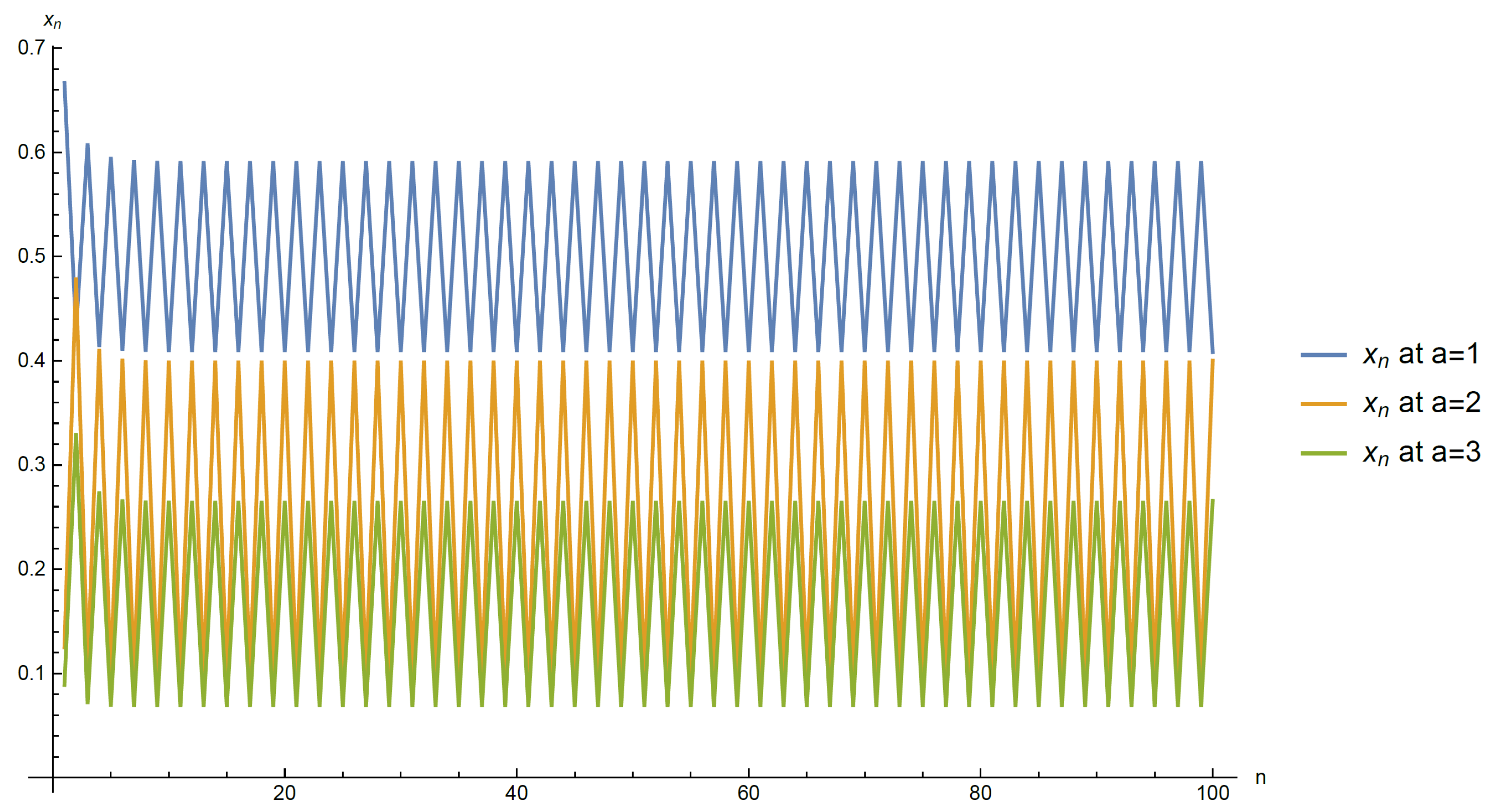
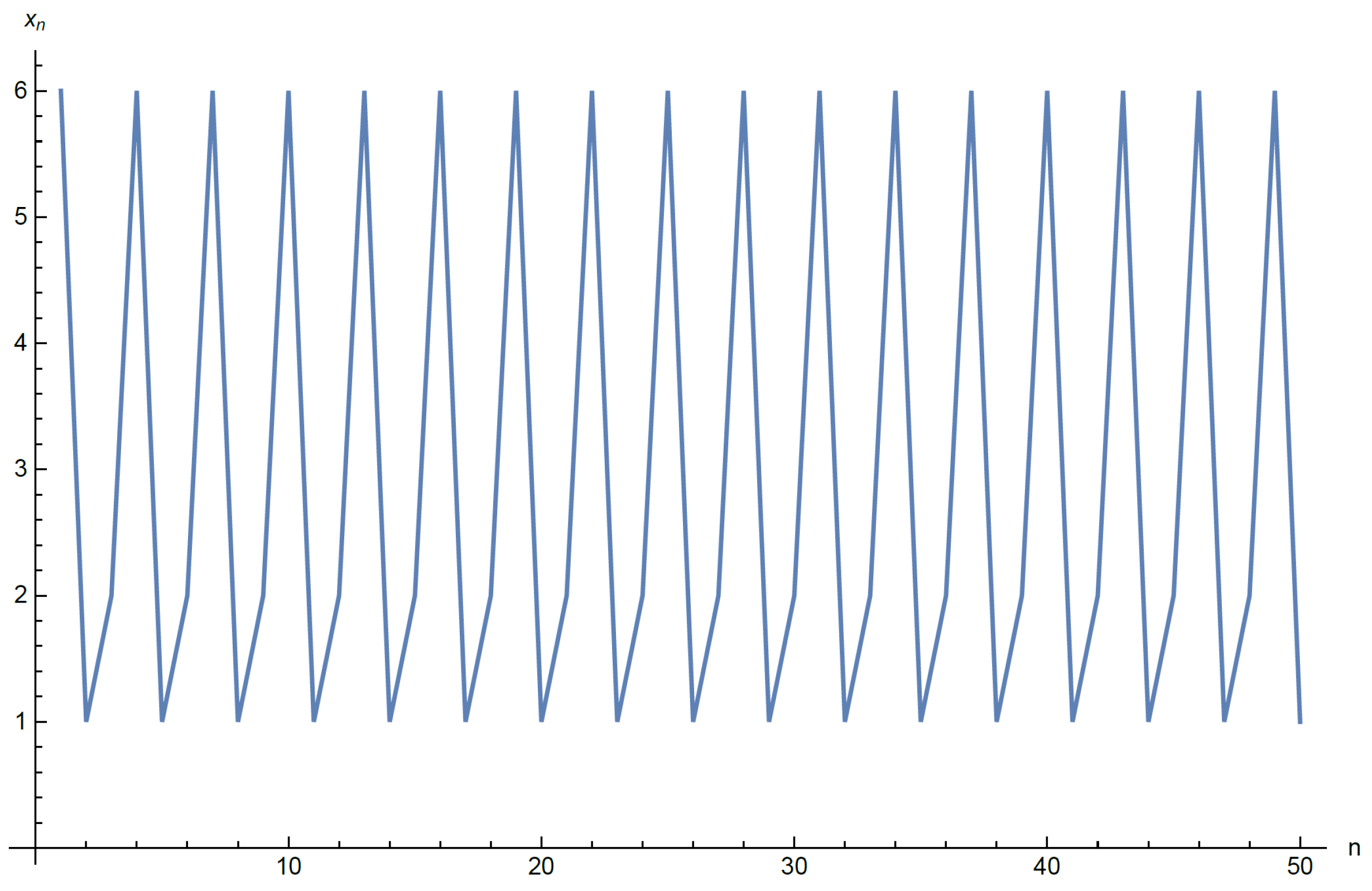
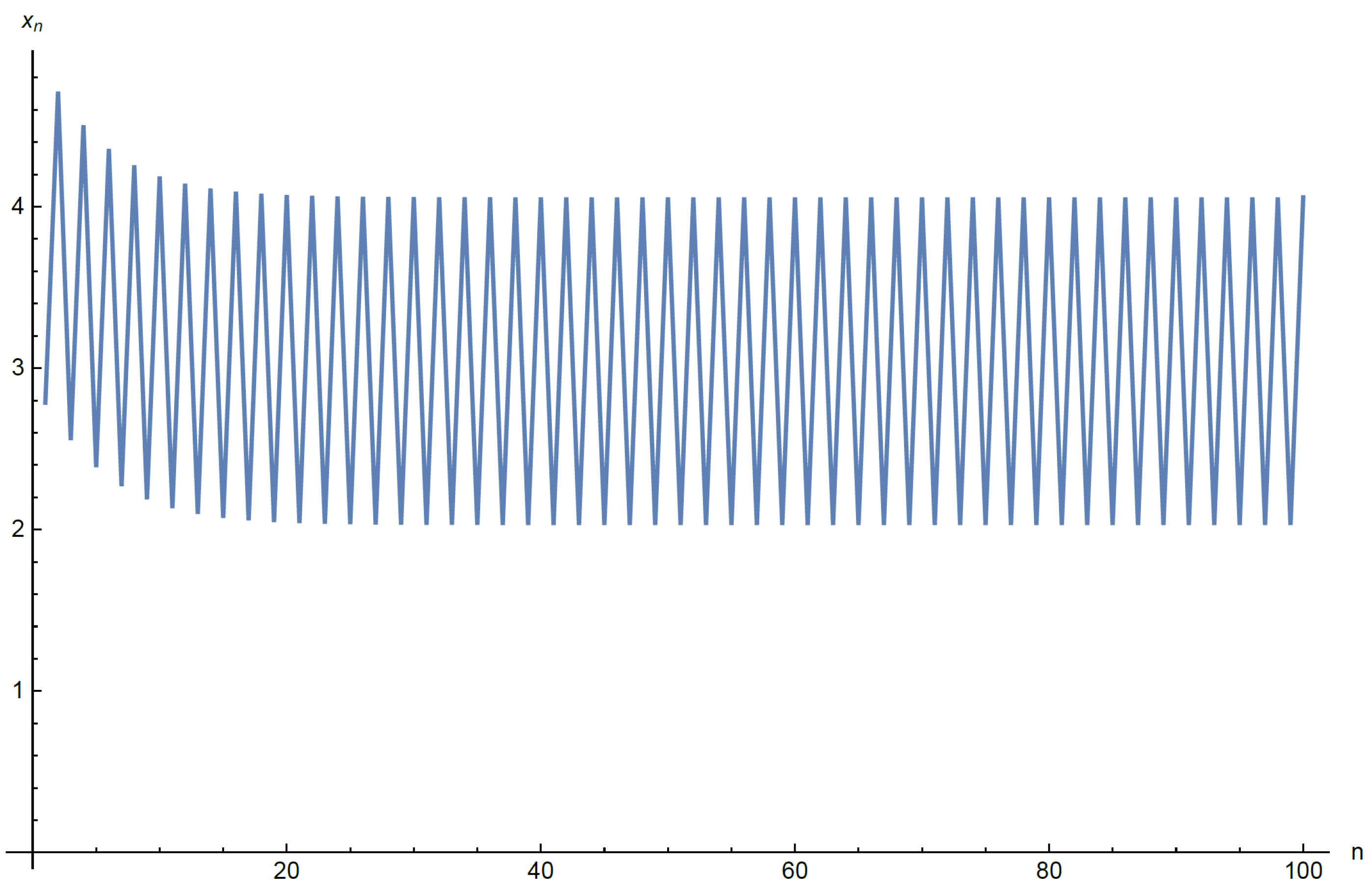
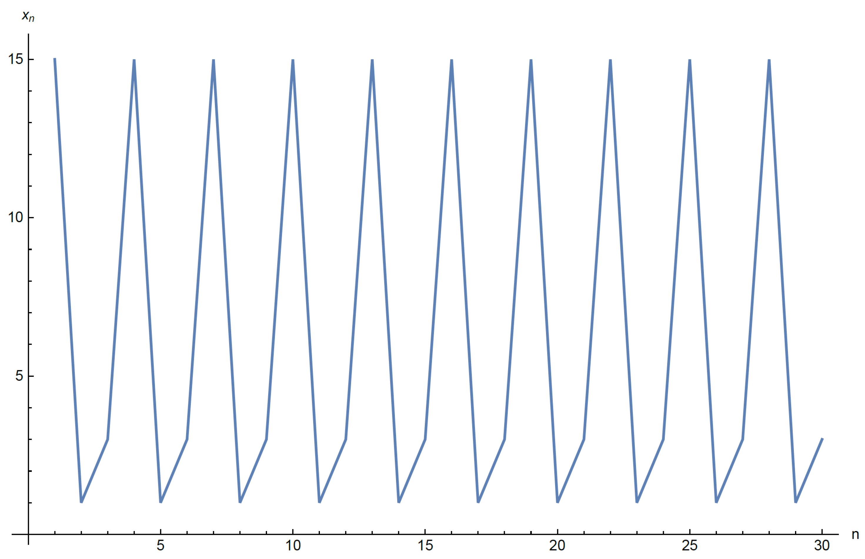
3.3. Examples and Numerical Simulations

In this part, we provide some examples that support the previous theoretical results. Examples are presented later, including what has been studied and what has not been studied before.

3.3.1. Special Case 1

Consider the DIE
u n + 1 = a u n 1 b u n + c u n 1 ,
where a , b , and c are positive real numbers. Using the substitution u n = a b z n , DIE (20) reduces to z n + 1 = c b + z n 1 z n , and this equation has been studied in [34].
It is easy to notice that P t , s = b a t + c a s is homogenous with degree o n e . Using our previous results, the following information can be obtained
  • DIE (20) has a prime period-two solution ⟺ b = c .
  • The positive EQP of DIE (20) is u e = a / b + c .
  • The EQP u e of DIE (20) is locally asymptotically stable (sink) if b < c .
  • If b < c , then EQP of DIE (20) is globally asymptotically stable.
  • We note that P l , 1 = 1 a c + 1 a b l c / a . Then, all solutions of DIE (20) are bounded if c > a .

3.3.2. Special Case 2

Consider the DIE
u n + 1 = u n 1 exp a b u n u n 1 c u n 1 u n ,
where a , b and c are real numbers. It is easy to notice that
P t , s = exp a + b t s + c s t
is homogenous with degree z e r o .
  • DIE (21) has a prime period-two solution ⟺ there is a l R + / 1 such that
    b l + c 1 l = b 1 l + c l ,
    i.e., b = c < 0 , see Figure 3.
  • DIE (21) has a prime period-three solution ⟺ there is a l , l R + / 1 such that
    b k 2 + a k + c = k ln k l , b l 2 + a l + c = l ln k , c k 2 + a k l + b l 2 = k l ln l ,
    see Figure 4.
  • Assume that b , c R + . We note that P l , 1 = e a + b l + c l e a . Then, every solution of DIE (22) converges to z e r o if a > 0 .

3.3.3. Special Case 3

Consider the DIE
u n + 1 = u n 1 a u n 2 + b u n u n 1 + c u n 1 2 ,
where a , b and c are real numbers, and one of them is not equal to zero at least. It is easy to notice that
P t , s = a t 2 + b ts + c s 2
is homogenous with degree two.
  • DIE (22) has a prime period-two solution ⟺ there is a l R + / 1 such that
    a c l 2 1 = 0
    i.e., a = c , see Figure 5.
  • DIE (22) has a prime period-three solution ⟺ there is a l , l R + / 1 such that
    c + a l 2 + b l c l a k 2 l b k l = 0 , a a k l 3 b k l 2 + c k 2 l 2 + b k l c k l = 0 , a c k l 2 a k 3 l 2 b k 2 l 2 + c k 2 l 2 + b k l = 0 ,
    see Figure 6.
  • The positive EQP of DIE (22) is
    u e = 1 a + b + c , a + b + c > 0 .
  • The EQP u e of DIE (22) is locally asymptotically stable (sink) if
    2 a + b < b + 2 c < 2 a + b + c .
    If a , b , and c are positive, then u e is locally asymptotically stable (sink) if a < c , is a saddle point if c < a , and is a nonhyperbolic point if a = c , see Figure 7.

4. Conclusions

Our interest in this work was centered on the examination of some features of solutions to the general DIE (1). We considered the periodic behavior, stability, and boundedness of solutions to DIE (1). In detail, we fulfilled the sufficient and necessary conditions for the existence of periodic solutions with periods two and three. We then obtained a complete perception of the local stability of the EQPs for DIE (1). Moreover, we presented a number of lemma and theorems that discuss the global stability and boundedness of the studied equation. Finally, we obtained many properties of the solutions for some special cases of the studied equation, and we showed numerical simulations of their solutions.
Studying the qualitative behavior of the general DIEs may significantly contribute to eliciting the characteristics of the solutions of some new models that appear as a result of scientific and technological development in various fields. It is interesting, as an extension of our results in this work, to study the qualitative properties of solutions to the general DIE u n + 1 = K u n , u n 1 , where K = G P t , s is a homothetic function.

Author Contributions

Conceptualization, O.M. and A.A.A.; methodology, O.M. and A.A.A.; formal analysis, O.M. and A.A.A.; investigation, O.M. and A.A.A.; writing—original draft preparation, O.M. and A.A.A.; writing—review and editing, O.M. All authors have read and agreed to the published version of the manuscript.

Funding

This research received no external funding.

Acknowledgments

The authors gratefully acknowledge Qassim University, represented by the Deanship of Scientific Research, on the financial support for this research under the number (COS-2022-1-1-J-27924) during the academic year 1444 AH/2022 AD.

Conflicts of Interest

The authors declare no conflict of interest.

References

  1. Kiguradze, I.T.; Chaturia, T.A. Asymptotic Properties of Solutions of Nonatunomous Ordinary Differential Equations; Kluwer Academic Publishers: Drodrcht, The Netherlands, 1993. [Google Scholar]
  2. Agarwal, R.P. Difference Equations and Inequalities, Theory, Methods and Applications, 2nd ed.; Marcel Dekker: New York, NY, USA, 2000. [Google Scholar]
  3. Ahlabrandt, C.D.; Peterson, A.C. Discrete Hamiltonian Systems: Difference Equations, Continued Fractions and Reccati Equations; Kluwer Academic Publishers: Drodrcht, The Netherlands, 1996. [Google Scholar]
  4. Elaydi, S. An Introduction to Difference Equations; Springer: New York, NY, USA, 1999. [Google Scholar]
  5. Sharkovsky, A.N.; Maistrenko, Y.L.; Romanenko, E.Y. Difference Equations and Their Applications; Springer: Dordrecht, The Netherlands, 1993. [Google Scholar]
  6. Diekmann, O.; Verduyn Lunel, S.M.; Gils, S.A.; Walther, H.-O. Delay Equations, Functional, Complex and Nonlinear Analysis; Springer: New York, NY, USA, 1995. [Google Scholar]
  7. Kolmonovskii, V.; Myshkis, A. Introduction to the Theory and Applications of Functional Differential Equations; Kluwer Academic Publishers: Drodrcht, The Netherlands, 1999. [Google Scholar]
  8. Kelley, W.G.; Peterson, A.C. Difference Equations; An Introduction with Applications, 2nd ed.; Academic Press: New York, NY, USA, 2000. [Google Scholar]
  9. Allman, E.S.; Rhodes, J.A. Mathematical Models in Biology: An Introduction; Cambridge University Press: New York, NY, USA, 2003. [Google Scholar]
  10. Beverton, R.J.H.; Holt, S.J. On the Dynamics of Exploited Fish Populations; Springer: Dordrecht, The Netherlands, 1993; Volume 11. [Google Scholar]
  11. Cooke, K.L.; Calef, D.F.; Level, E.V. Stability or chaos in discrete epidemic models. In Nonlinear Systems and Applications; Academic Press: New York, NY, USA, 1977. [Google Scholar]
  12. Cull, P.; Flahive, M.; Robson, R. Difference Equations, From Rabbits to Chaos; Undergraduate Texts in Mathematics; Springer: New York, NY, USA, 2005. [Google Scholar]
  13. Din, Q. A novel chaos control strategy for discrete-time Brusselator models. J. Math. Chem. 2018, 56, 3045–3075. [Google Scholar] [CrossRef]
  14. Din, Q. Bifurcation analysis and chaos control in discrete-time glycolysis models. J. Math. Chem. 2018, 56, 904–931. [Google Scholar] [CrossRef]
  15. Din, Q.; Elsayed, E.M. Stability analysis of a discrete ecological model. Comput. Ecol. Softw. 2014, 4, 89–103. [Google Scholar]
  16. Elsayed, E.M. New method to obtain periodic solutions of period two and three of a rational difference equation. Nonlinear Dyn. 2015, 79, 241–250. [Google Scholar] [CrossRef]
  17. Moaaz, O. Comment on New method to obtain periodic solutions of period two and three of a rational difference equation [Nonlinear Dyn 79: 241–250]. Nonlinear Dyn. 2017, 88, 1043–1049. [Google Scholar] [CrossRef]
  18. Kulenovic, M.R.S.; Ladas, G. Dynamics of Second Order Rational Difference Equations with Open Problems and Conjectures; Chapman & Hall/CRC Press: Boca Raton, FL, USA, 2001. [Google Scholar]
  19. Kuruklis, S.; Ladas, G. Oscillation and global attractivity in a discrete delay logistic model. Quart. Appl. Math. 1992, 50, 227–233. [Google Scholar] [CrossRef] [Green Version]
  20. Pielou, E.C. An Introduction to Mathematical Ecology; John Wiley & Sons: New York, NY, USA, 1965. [Google Scholar]
  21. May, R.M. Nonlinear problems in ecology and resource management. Chaotic Behav. Determ. Syst. 1983, 389–439. [Google Scholar]
  22. Kuang, Y.K.; Cushing, J.M. Global stability in a nonlinear difference-delay equation model of flour beetle population growth. J. Differ. Equ. Appl. 1996, 2, 31–37. [Google Scholar] [CrossRef]
  23. Stevo, S. The recursive sequence un+1 = g(un,un−1)/(A + un). Appl. Math. Lett. 2002, 15, 305–308. [Google Scholar] [CrossRef] [Green Version]
  24. Karakostas, G.L.; Stevic, S. On the recursive sequence un+1 = α + unk/f(un,un−1,⋯,unk+1). Demonstr. Math. 2005, 38, 595. [Google Scholar]
  25. Sun, S.; Xi, H. Global behavior of the nonlinear difference equation un+1 = f(un−s,un−t). J. Math. Anal. Appl. 2005, 311, 760–765. [Google Scholar] [CrossRef] [Green Version]
  26. Moaaz, O. Dynamics of difference equation un+1 = f(unl,unk). Adv. Differ. Equ. 2018, 2018, 447. [Google Scholar] [CrossRef] [Green Version]
  27. Elsayed, E.M.; Alofi, B.S. Dynamics and solutions structures of nonlinear system of difference equations. Math. Method. Appl. Sci. 2022, 2022, 1–18. [Google Scholar] [CrossRef]
  28. Elsayed, E.M.; Aloufi, B.S.; Moaaz, O. The behavior and structures of solution of fifth-order rational recursive sequence. Symmetry 2022, 14, 641. [Google Scholar] [CrossRef]
  29. Elsayed, E.M.; Alofi, B.S. The periodic nature and expression on solutions of some rational systems of difference equations. Alex. Eng. J. 2023, 74, 269–283. [Google Scholar] [CrossRef]
  30. Al-Basyouni, K.S.; Elsayed, E.M. On some solvable systems of some rational difference equations of third order. Mathematics 2023, 11, 1047. [Google Scholar] [CrossRef]
  31. Kara, M.; Yazlik, Y. On the solutions of three-dimensional system of difference equations via recursive relations of order two and applications. J. Appl. Anal. Comput. 2022, 12, 736–753. [Google Scholar] [CrossRef] [PubMed]
  32. Al-Khedhairi, A.; Elsadany, A.A.; Elsonbaty, A. On the dynamics of a discrete fractional-order cournot–bertrand competition duopoly game. Math. Probl. Eng. 2022, 2022, 8249215. [Google Scholar] [CrossRef]
  33. Khaliq, A.; Mustafa, I.; Ibrahim, T.F.; Osman, W.M.; Al-Sinan, B.R.; Dawood, A.A.; Juma, M.Y. Stability and bifurcation analysis of fifth-order nonlinear fractional difference equation. Fractal Fract. 2023, 7, 113. [Google Scholar] [CrossRef]
  34. Amleh, A.M.; Georgiou, D.A.; Grove, E.A.; Ladas, G. On the recursive sequence un+1 = α+un−1/un. J. Math. Anal. Appl. 1999, 233, 790–798. [Google Scholar] [CrossRef] [Green Version]
Figure 1. Periodic solutions of DIE (8) at a = b = 1 , 2 , or 3 .
Axioms 12 00598 g001
Figure 2. Prime period-three solution of DIE (12).
Axioms 12 00598 g002
Figure 3. Periodic solutions of DIE (21) at a = 1 , and b = c = 2 / 5 .
Axioms 12 00598 g003
Figure 4. Periodic solutions of DIE (21) at a = 8.7829 , b = 1.9489 , and c = 0.684 16 .
Axioms 12 00598 g004
Figure 5. Periodic solutions of DIE (22) at b = 2 , and a = c = 1 .
Axioms 12 00598 g005
Figure 6. Periodic solutions of DIE (22) at a = 38 41 , b = 196 123 , and c = 1 .
Axioms 12 00598 g006
Figure 7. Stability behavior of solutions (22).
Axioms 12 00598 g007
Disclaimer/Publisher’s Note: The statements, opinions and data contained in all publications are solely those of the individual author(s) and contributor(s) and not of MDPI and/or the editor(s). MDPI and/or the editor(s) disclaim responsibility for any injury to people or property resulting from any ideas, methods, instructions or products referred to in the content.

