Dynamics of a Fractional-Order COVID-19 Epidemic Model with Quarantine and Standard Incidence Rate

Abstract

In this paper, we propose a fractional-order COVID-19 epidemic model with a quarantine and standard incidence rate using the Caputo fractional-order derivative. The model consists of six classes: susceptible (S), exposed (E), infected (I), quarantined (Q), recovered (R), and deceased (M). In our proposed model, we simultaneously consider the recovery rate and quarantine rate of infected individuals, which has not been considered in other fractional-order COVID-19 epidemic models. Furthermore, we consider the standard incidence rate in the model. For our proposed model, we prove the existence, uniqueness, non-negativity, and boundedness of the solution. The model has two equilibrium points: disease-free equilibrium and endemic equilibrium. Implementing the spectral radius of the next-generation matrix, we obtain the basic reproduction number (${\mathcal{R}}_0$). The disease-free equilibrium always exists and is locally and globally asymptotically stable only if ${\mathcal{R}}_0<1$. On the other hand, endemic equilibrium exists and is globally asymptotically stable if ${\mathcal{R}}_0>1$. Our numerical simulation confirms the stability properties of the equilibrium. The smaller the order of the derivative, the slower the convergence of the solution of the model. Both the recovery rate and quarantine rate of the infected class are important parameters determining the stability of the equilibrium point. Based on parameter estimation from COVID-19 data in Indonesia, the fractional-order model has better performance than the first-order model for both the calibration and 20-day forecasting of confirmed daily active cases of COVID-19.

1. Introduction

Coronavirus Disease 2019, or COVID-19, is an acute respiratory disease that was first indicated in Wuhan Province, China, in 2019 [1]. COVID-19 is an infectious disease caused by infection with the SARS-CoV-2 virus [2]. Symptoms of this disease are fever, flu, cough, pneumonia, and other symptoms that cause complications such as asthma [1,3]. COVID-19 can spread quickly, and the total number of cases reached 624 million cases in the world [4]. The number of cases is also influenced by the variant of the COVID-19 virus. In general, there are five variants of COVID-19 virus: Alpha, Beta, Gamma, Delta, and Omicron [5,6]. Various studies on how COVID-19 is transmitted have been described in [7,8,9]. The mechanism of transmission most often occurs through droplets, directly or indirectly [2,10,11]. To prevent the spread of the virus, quarantine is an effective intervention [11,12,13]. Quarantine causes infected individuals to lose contact with other individuals, which can wipe out the transmission of the disease [14]. Thus, the mechanism of transmission with quarantine interventions is important to understand and study further.

Mathematical modeling is an approximation used to understand the mechanism of transmission and current state of COVID-19 [15]. If COVID-19 data are sufficient, then the forecasting of COVID-19 via parameter estimation is very helpful for policy makers, as was conducted in [16,17,18]. Otherwise, the dynamics of an epidemic model can provide conditions that lead to an endemic disease. Some researchers have studied the COVID-19 pandemic via the dynamics of mathematical models, such as in [15,19,20]. The mathematical model for a disease epidemic is basically represented by first-order differential equations.

Some researchers have developed COVID-19 epidemic models. Zeb et al. [21] proposed a COVID-19 epidemic model with a quarantined class. The paper of Zeb et al. [21] focuses on the dynamics of the COVID-19 epidemic model. In the model, there is an assumption that exposed individuals can transmit the COVID-19 virus. The current literature shows that an exposed individual is an infected individual but does not always transmit the virus [22,23]. Furthermore, the mortality of COVID-19 is not considered in the model of Zeb et al. [21]. Another COVID-19 epidemic model was proposed by López and Rodó [24] with a quarantined class and protected class. They focus on the calibration of COVID-19 data in Italy and Spain. In their model, there is an assumption that the death class only comes from the quarantined class. Musafir et al. [15] stated that infected individuals can also cause death from COVID-19. In both models, the incidence rate used is bilinear, with a maximum proportion of the total of living classes. A recent model has been proposed to resolve the weak assumption for these models. The proposed model by Darti et al. [25] assumes that the exposed class is not contagious and the infected class may induce death from COVID-19. These assumptions improve the proposed models by Zeb et al. [21] and López and Rodó [24]. All three models are represented by nonlinear first-order differential equations.

In recent decades, fractional calculus has been developed to provide some integral and derivative options [26,27]. A fractional derivative is a non-local operator, which means the rate of the function depends on previous histories from the initial value, which is called the memory effect [26]. In epidemiology, the future spread of a disease depends on recent and previous conditions because of the impact of both heredity and history on individual habits [28]. Hence, the fractional derivative is more realistic than the integer derivative. Moreover, some researchers, such as [2,20,29,30], state that fractional derivatives provide better accuracy and flexibility than integer derivatives. There are two types of fractional operators obtained by generalizing the integer-order derivative, namely, the Riemann–Liouville operator and the Caputo operator [31]. Li et al. [32] show that the Caputo operator is better than the Riemann–Liouville operator in terms of applied mathematics.

Recently, many researchers have proposed a fractional-order COVID-19 epidemic model. Yadav et al. [33] introduced a fractional-order SEIR-type model by dividing the infected class into two subclasses: the infected subclass without symptoms and the infected subclass with symptoms. The proposed model was analyzed dynamically and solved using q-homotopy analysis with the Sumudu transform method. With the increasing incidences of COVID-19, various measures have been taken by many countries to control the spread of COVID-19. One of the well-known preventive measures is a lockdown. The impact of lockdowns has been modeled by [34], i.e., by considering a fractional-order SI-type epidemic model where the population is split into the subpopulation not under lockdown and the subpopulation under lockdown. In [35], the authors considered a fractional SEIR model incorporating public risk awareness and the spread of disease caused by both human-to-human and zoonotic transmissions. Then, in [36], the authors extended the model of [33] by considering the classes of quarantine, isolation, and environmental impacts.

We notice that although the fractional-order COVID-19 epidemic models above were derived based on the Caputo fractional derivative operator, they did not pay attention to the inconsistency in the time dimension. Such dimensional inconsistency is caused by replacing the first-order derivative with a Caputo fractional-order derivative. Moreover, none of those models have considered the effects of fractional-order derivatives. In this study, we propose a fractional-order COVID-19 epidemic model by including the dimensional issue. We implement the proposed model using real COVID-19 data. Since the available data only consist of the confirmed active COVID-19 cases (the infected subclass), without noting whether this is with or without symptoms, we consider a simpler model than proposed by [36]. For this aim, we modify the COVID-19 epidemic model proposed by Darti et al. [25] to a fractional-order model with a Caputo fractional operator. The proposed COVID-19 epidemic model by Darti et al. [25] is given as follows, with the parameter definitions listed in

Table 1. Description of variables and parameters.

Parameter	Description
$S\left(t\right)$	Susceptible class
$E\left(t\right)$	Exposed class
$I\left(t\right)$	Infected class
$Q\left(t\right)$	Quarantined class
$R\left(t\right)$	Recovered class
$M\left(t\right)$	Death class
$N\left(t\right)$	Total of living class
$\hat{\Lambda }$	Recruitment rate
$\hat{\beta }$	Rate of disease transmission
$\hat{\mu }$	Natural death rate
$\hat{\gamma }$	Incubation rate
$\hat{\sigma }$	Quarantine rate
$\hat{\eta }$	Recovery rate of infected class
$\hat{\delta }$	Mortality rate of infected class
$\hat{\vartheta }$	Recovery rate of quarantined class
$\hat{\kappa }$	Mortality rate of quarantined class

:

$$\begin{array}{ccc}\hfill \frac{dS\left(t\right)}{dt}\hfill & =& \hat{\Lambda }-\frac{\hat{\beta }S\left(t\right)I\left(t\right)}{N\left(t\right)}-\hat{\mu }S\left(t\right),\hfill \\ \hfill \frac{dE\left(t\right)}{dt}\hfill & =& \frac{\hat{\beta }S\left(t\right)I\left(t\right)}{N\left(t\right)}-(\hat{\gamma }+\hat{\mu })E\left(t\right),\hfill \\ \hfill \frac{dI\left(t\right)}{dt}\hfill & =& \hat{\gamma }E\left(t\right)-(\hat{\sigma }+\hat{\eta }+\hat{\delta }+\hat{\mu })I\left(t\right),\hfill \\ \hfill \frac{dQ\left(t\right)}{dt}\hfill & =& \hat{\sigma }I\left(t\right)-(\hat{\vartheta }+\hat{\kappa }+\hat{\mu })Q\left(t\right),\hfill \\ \hfill \frac{dR\left(t\right)}{dt}\hfill & =& \hat{\eta }I\left(t\right)+\hat{\vartheta }Q\left(t\right)-\hat{\mu }R\left(t\right),\hfill \\ \hfill \frac{dM\left(t\right)}{dt}\hfill & =& \hat{\delta }I\left(t\right)+\hat{\kappa }Q\left(t\right).\hfill \end{array}$$

(1)

In this study, we first propose the fractional-order COVID-19 epidemic model in Section 2. The basic properties of the proposed model are presented in Section 3 and Section 4. The equilibrium points of the model and their stability are given in Section 5 and Section 6, respectively. To measure how sensitive the model parameters are to COVID-19 transmission, in Section 7, we provide a sensitivity analysis. In Section 8, we numerically simulate the properties of the dynamic analysis of our proposed model. The numerical solutions are obtained by adopting the predictor–corrector scheme proposed by [37]. In Section 9, we implement our proposed model using COVID-19 data in Indonesia. Parameter estimation is performed using the nonlinear least square method. This can be achieved using MATLAB’s built-in function lsqcurvefit. Here, we minimize the squared error between numerical solutions for infected subpopulations and confirmed active daily data. Finally, we remark upon the conclusions of this study in Section 10.

2. Model Formulation

We modify the model proposed by Darti et al. [25] to a fractional-order model with the Caputo operator. The Caputo fractional operator is given as follows.

Definition 1 

([38]). Let $t\ge 0$ and $\alpha \in (0,1)$. The Riemann–Liouville integral of order α is defined by

$${}^{RL}{\mathfrak{I}}_t^{\alpha }x\left(t\right)={}^{RL}{D}_t^{-\alpha }x\left(t\right)=\frac{1}{\Gamma \left(\alpha \right)}{\int }_0^t{(t-\tau )}^{\alpha -1}x\left(\tau \right)d\tau$$

where $x\in C^n\left([0,\infty ),\mathbb{R}\right)$ and $\Gamma (·)$ is a Gamma function.

Definition 2 

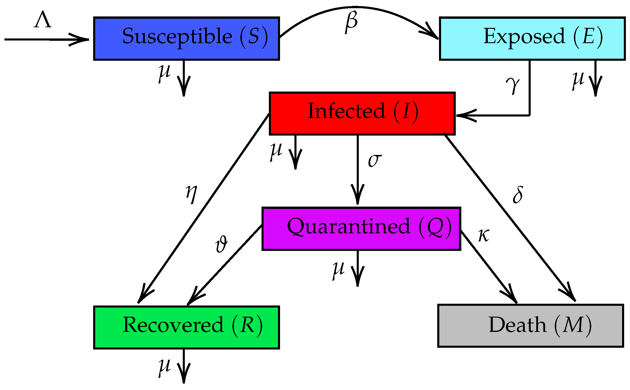
([38]). Let $t\ge 0$ and $\alpha \in (0,1)$. The Caputo derivative of order α is defined by

$${}^{\mathcal{C}}{D}_t^{\alpha }x\left(t\right)=\frac{1}{\Gamma (1-\alpha )}{\int }_0^t{(t-\tau )}^{-\alpha }{x}^{\prime }\left(\tau \right)d\tau ,$$

where $x\in C^n\left([0,\infty ),\mathbb{R}\right)$.

Our proposed model has five population classes: the susceptible class (S), the exposed class (E), the infected class (I), the quarantined class (Q), the recovered class (R), and the death class (M). We define variable N as the total of living individuals, which is denoted as $N=S+E+I+Q+R$. The individuals of the susceptible class (S) who are in close contact with infected individuals have the potential to be exposed individuals. The exposed class is infected but not yet infectious. After the incubation period of the virus, exposed individuals move to the infected class (I), which is composed of the infected individuals. The infected individuals can be either quarantined, recovered, or dead from illness. The quarantined individuals (Q) can be either recovered or dead. The interaction of all classes is depicted in Figure 1. The proposed fractional-order SEIQRM model with the Caputo derivative operator is derived by replacing the first-order derivatives in the SEIQRM model (1) with the Caputo fractional derivatives. However, if we perform this step, then there is a time-dimensional inconsistency on both sides of all the equations because the fractional derivatives of order $\alpha$ have the dimension of ${\left(time\right)}^{-\alpha }$. To handle the dimension inconsistency, we rescale the parameters and obtain the following fractional-order SEIQRM model:

$$\begin{array}{ccc}\hfill {}^{\mathcal{C}}{D}_t^{\alpha }S\left(t\right)\hfill & =& \Lambda -\frac{\beta S\left(t\right)I\left(t\right)}{N\left(t\right)}-\mu S\left(t\right),\hfill \\ \hfill {}^{\mathcal{C}}{D}_t^{\alpha }E\left(t\right)\hfill & =& \frac{\beta S\left(t\right)I\left(t\right)}{N\left(t\right)}-(\gamma +\mu )E\left(t\right),\hfill \\ \hfill {}^{\mathcal{C}}{D}_t^{\alpha }I\left(t\right)\hfill & =& \gamma E\left(t\right)-(\sigma +\eta +\delta +\mu )I\left(t\right),\hfill \\ \hfill {}^{\mathcal{C}}{D}_t^{\alpha }Q\left(t\right)\hfill & =& \sigma I\left(t\right)-(\vartheta +\kappa +\mu )Q\left(t\right),\hfill \\ \hfill {}^{\mathcal{C}}{D}_t^{\alpha }R\left(t\right)\hfill & =& \eta I\left(t\right)+\vartheta Q\left(t\right)-\mu R\left(t\right),\hfill \\ \hfill {}^{\mathcal{C}}{D}_t^{\alpha }M\left(t\right)\hfill & =& \delta I\left(t\right)+\kappa Q\left(t\right),\hfill \end{array}$$

(2)

where $\Lambda ={\hat{\Lambda }}^{\alpha },\beta ={\hat{\beta }}^{\alpha },\mu ={\hat{\mu }}^{\alpha },\gamma ={\hat{\gamma }}^{\alpha },\sigma ={\hat{\sigma }}^{\alpha },\eta ={\hat{\eta }}^{\alpha },\delta ={\hat{\delta }}^{\alpha },\vartheta ={\hat{\vartheta }}^{\alpha }$, and $\kappa ={\hat{\kappa }}^{\alpha }$.

3. Existence and Uniqueness of Solution

In this section, we explicitly prove the existence and uniqueness of the solution of model (2).

Theorem 1. 

Let the initial values of model (2) be non-negative. The model (2) has a unique solution in ${\mathbb{R}}_{+}^5$ for all $t\ge 0$.

Proof. 

If the right-hand side of model (2) is written by

$$\begin{array}{ccc}\hfill f_1& =& \Lambda -\frac{\beta S\left(t\right)I\left(t\right)}{N\left(t\right)}-\mu S\left(t\right),\hfill \\ \hfill f_2& =& \frac{\beta S\left(t\right)I\left(t\right)}{N\left(t\right)}-(\gamma +\mu )E\left(t\right),\hfill \\ \hfill f_3& =& \gamma E\left(t\right)-(\sigma +\eta +\delta +\mu )I\left(t\right),\hfill \\ \hfill f_4& =& \sigma I\left(t\right)-(\vartheta +\kappa +\mu )Q\left(t\right),\hfill \\ \hfill f_5& =& \eta I\left(t\right)+\vartheta Q\left(t\right)-\mu R\left(t\right),\hfill \end{array}$$

since $\frac{I}{N}\le 1$, we find for every $S,\overline{S}\in {\mathbb{R}}_{+}^5$ that

$$\begin{array}{c}\hfill \parallel f_1(S,t)-f_1(\overline{S},t)\parallel =∥-\frac{\beta SI}{N}-\mu S+\frac{\beta \overline{S}I}{N}+\mu \overline{S}∥\le p_1\parallel S-\overline{S}\parallel ,\end{array}$$

with $p_1=(\beta +\mu )$. In the same way, we can show that

$$\begin{array}{c}\hfill \parallel f_2(E,t)-f_2(\overline{E},t)\parallel \le p_2\parallel E-\overline{E}\parallel ,\\ \hfill \parallel f_3(I,t)-f_3(\overline{I},t)\parallel \le p_3\parallel I-\overline{I}\parallel ,\\ \hfill \parallel f_4(Q,t)-f_4(\overline{Q},t)\parallel \le p_4\parallel Q-\overline{Q}\parallel ,\\ \hfill \parallel f_5(R,t)-f_5(\overline{R},t)\parallel \le p_5\parallel R-\overline{R}\parallel ,\end{array}$$

where $p_2=\gamma +\mu$, $p_3=\sigma +\eta +\delta +\mu$, $p_4=\vartheta +\kappa +\mu$, $p_5=\mu$. It is clear that if $0<p_i<1$, $i=1,2,\dots ,5$, then all kernels of $f_i$ contract and satisfy the Lipschitz condition.

If both sides of model (2) are integrated by Definition 1, then we obtain

$$\begin{array}{ccc}\hfill S\left(t\right)-S\left(0\right)& =& \hfill \frac{1}{\Gamma \left(\alpha \right)}{\int }_0^t{(t-\tau )}^{\alpha -1}{f}_1\left(S,\tau \right)d\tau ,\hfill \\ \hfill E\left(t\right)-E\left(0\right)& =& \hfill \frac{1}{\Gamma \left(\alpha \right)}{\int }_0^t{(t-\tau )}^{\alpha -1}{f}_2\left(E,\tau \right)d\tau ,\hfill \\ \hfill I\left(t\right)-I\left(0\right)& =& \hfill \frac{1}{\Gamma \left(\alpha \right)}{\int }_0^t{(t-\tau )}^{\alpha -1}{f}_3\left(I,\tau \right)d\tau ,\hfill \\ \hfill Q\left(t\right)-Q\left(0\right)& =& \hfill \frac{1}{\Gamma \left(\alpha \right)}{\int }_0^t{(t-\tau )}^{\alpha -1}{f}_4\left(Q,\tau \right)d\tau ,\hfill \\ \hfill R\left(t\right)-R\left(0\right)& =& \hfill \frac{1}{\Gamma \left(\alpha \right)}{\int }_0^t{(t-\tau )}^{\alpha -1}{f}_5\left(R,\tau \right)d\tau .\hfill \end{array}$$

(3)

Hence, we obtain the iterative scheme

$$\begin{array}{ccc}\hfill S_n\left(t\right)& =& \hfill S\left(0\right)+\frac{1}{\Gamma \left(\alpha \right)}{\int }_0^t{(t-\tau )}^{\alpha -1}{f}_1\left(S_{n-1},\tau \right)d\tau ,\hfill \\ \hfill {\mathcal{E}}_n\left(t\right)& =& \hfill E\left(0\right)+\frac{1}{\Gamma \left(\alpha \right)}{\int }_0^t{(t-\tau )}^{\alpha -1}{f}_2\left({\mathcal{E}}_{n-1},\tau \right)d\tau ,\hfill \\ \hfill I_n\left(t\right)& =& \hfill I\left(0\right)+\frac{1}{\Gamma \left(\alpha \right)}{\int }_0^t{(t-\tau )}^{\alpha -1}{f}_3\left(I_{n-1},\tau \right)d\tau ,\hfill \\ \hfill Q_n\left(t\right)& =& \hfill Q\left(0\right)+\frac{1}{\Gamma \left(\alpha \right)}{\int }_0^t{(t-\tau )}^{\alpha -1}{f}_4\left(Q_{n-1},\tau \right)d\tau ,\hfill \\ \hfill R_n\left(t\right)& =& \hfill R\left(0\right)+\frac{1}{\Gamma \left(\alpha \right)}{\int }_0^t{(t-\tau )}^{\alpha -1}{f}_5\left(R_{n-1},\tau \right)d\tau .\hfill \end{array}$$

(4)

Next, we construct a recursive formulation based on the Equation (4) as follows:

$$\begin{array}{ccc}\hfill {\psi }_{1n}\left(t\right)& =& S_n\left(t\right)-S_{n-1}\left(t\right)=\frac{1}{\Gamma \left(\alpha \right)}{\int }_0^t{(t-\tau )}^{\alpha -1}\left(f_1(S_{n-1},\tau )-f_1(S_{n-2},\tau )\right)d\tau ,\hfill \\ \hfill {\psi }_{2n}\left(t\right)& =& {\mathcal{E}}_n\left(t\right)-{\mathcal{E}}_{n-1}\left(t\right)=\frac{1}{\Gamma \left(\alpha \right)}{\int }_0^t{(t-\tau )}^{\alpha -1}\left(f_2({\mathcal{E}}_{n-1},\tau )-f_2({\mathcal{E}}_{n-2},\tau )\right)d\tau ,\hfill \\ \hfill {\psi }_{3n}\left(t\right)& =& I_n\left(t\right)-I_{n-1}\left(t\right)=\frac{1}{\Gamma \left(\alpha \right)}{\int }_0^t{(t-\tau )}^{\alpha -1}\left(f_3(I_{n-1},\tau )-f_3(I_{n-2},\tau )\right)d\tau ,\hfill \\ \hfill {\psi }_{4n}\left(t\right)& =& Q_n\left(t\right)-Q_{n-1}\left(t\right)=\frac{1}{\Gamma \left(\alpha \right)}{\int }_0^t{(t-\tau )}^{\alpha -1}\left(f_4(Q_{n-1},\tau )-f_4(Q_{n-2},\tau )\right)d\tau ,\hfill \\ \hfill {\psi }_{5n}\left(t\right)& =& R_n\left(t\right)-R_{n-1}\left(t\right)=\frac{1}{\Gamma \left(\alpha \right)}{\int }_0^t{(t-\tau )}^{\alpha -1}\left(f_5(R_{n-1},\tau )-f_5(R_{n-2},\tau )\right)d\tau .\hfill \end{array}$$

(5)

The norm of the first equation of (5) can be expressed as

$$\begin{array}{ccc}\hfill \parallel {\psi }_{1n}\left(t\right)\parallel & =& \parallel S_n\left(t\right)-S_{n-1}\left(t\right)\parallel \hfill \\ & =& ∥\frac{1}{\Gamma \left(\alpha \right)}{\int }_0^t{(t-\tau )}^{\alpha -1}\left(f_1(S_{n-1},\tau )-f_1(S_{n-2},\tau )\right)d\tau ∥\hfill \\ & \le & \frac{1}{\Gamma \left(\alpha \right)}{\int }_0^t{(t-\tau )}^{\alpha -1}∥f_1(S_{n-1},\tau )-f_1(S_{n-2},\tau )∥d\tau \hfill \\ & \le & \frac{p_1}{\Gamma \left(\alpha \right)}{\int }_0^t{(t-\tau )}^{\alpha -1}\parallel S_{n-1}\left(\tau \right)-S_{n-2}\left(\tau \right)\parallel d\tau \hfill \\ & =& \frac{p_1}{\Gamma \left(\alpha \right)}{\int }_0^t{(t-\tau )}^{\alpha -1}\parallel {\psi }_{1(n-1)}\left(\tau \right)\parallel d\tau \hfill \\ & =& {\left(\frac{p_{1}t}{\Gamma (\alpha +1)}\right)}^n\parallel S\left(0\right)\parallel .\hfill \end{array}$$

Similarly, we have

$$\begin{array}{c}\hfill \parallel {\psi }_{jn}\left(t\right)\parallel \le {\left(\frac{p_{1}t}{\Gamma (\alpha +1)}\right)}^n\parallel X_j\left(0\right)\parallel ,\mathrm{f}\mathrm{o}\mathrm{r} \mathrm{a}\mathrm{l}\mathrm{l} j=2,3,4,5,\end{array}$$

where $(X_1,X_2,X_3,X_4,X_5)=(S,E,I,Q,R)$. Assume that there is $t=T$ such that

$$\begin{array}{c}\hfill \frac{p_{j}T}{\Gamma (\alpha +1)}<1,\mathrm{f}\mathrm{o}\mathrm{r} \mathrm{a}\mathrm{l}\mathrm{l} j=1,2,\dots ,5.\end{array}$$

It is clear that for every $j=1,2,\dots ,5,\parallel {\psi }_{jn}\left(t\right)\parallel \to 0$ as $n\to \infty$. Therefore, the solution of model (2) exists; that is, it is constructed from the Equation (3).

Next, we show that every solution with the same initial value is unique. Suppose the model (2) has two different solutions with the same initial value, where the other solutions are denoted by $\hat{S}$, $\hat{E}$, $\hat{I}$, $\hat{Q}$, and $\hat{R}$. We obtain

$$\begin{array}{c}\hfill S\left(t\right)-\hat{S}\left(t\right)=\frac{1}{\Gamma \left(\alpha \right)}{\int }_0^t{(t-\tau )}^{\alpha -1}\left(f_1(S,\tau )-f_1(\hat{S},\tau )\right)d\tau .\end{array}$$

The norm of the above equation is

$$\begin{array}{c}\hfill \parallel S\left(t\right)-\hat{S}\left(t\right)\parallel \le \frac{1}{\Gamma \left(\alpha \right)}{\int }_0^t{(t-\tau )}^{\alpha -1}∥f_1(S,\tau )-f_1(\hat{S},\tau )∥,\end{array}$$

so that by using the Lipschitz condition, we obtain

$$\begin{array}{ccc}\hfill \parallel S\left(t\right)-\hat{S}\left(t\right)\parallel & \le & \frac{p_{1}T}{\Gamma (\alpha +1)}\parallel S\left(t\right)-\hat{S}\left(t\right)\parallel \hfill \\ \hfill \left(1-\frac{p_{j}T}{\Gamma (\alpha +1)}\right)\parallel S\left(t\right)-\hat{S}\left(t\right)\parallel & \le & 0.\hfill \end{array}$$

(6)

The inequality (6) is satisfied if and only if $\parallel S\left(t\right)-\hat{S}\left(t\right)\parallel =0$, which means $S\left(t\right)=\hat{S}\left(t\right)$. This leads to a contradiction, so that $S\left(t\right)$ is unique. In a similar way, we can show that $E\left(t\right)$, $I\left(t\right)$, $Q\left(t\right)$, and $R\left(t\right)$ are unique. □

4. Non-Negativity and Boundedness of the Solution

In this section, we show the non-negativity and boundedness of the solution of model (2). We also obtain the feasible region of model (2). The following theorem guarantees the non-negativity and boundedness of the solution.

Theorem 2. 

All solutions of model (2) subject to non-negative initial values are non-negative and ultimately bounded. The feasible region of model (2) is given by

$$\begin{array}{c}\hfill \mathsf{\Omega }=\left\{(S,E,I,Q,R)\in {\mathbb{R}}_{+}^5\cup \overrightarrow{0}:N\le \frac{\Lambda }{\mu }\right\}.\end{array}$$

Proof. 

We first show that S is non-negative. Assume $S<0$ for some $t>0$. Then, there is at least one $\tau >0$ such that

$$\begin{array}{c}\hfill S\left({\tau }^{-}\right)\ge 0,S\left(\tau \right)=0,S\left({\tau }^{+}\right)<0.\end{array}$$

From model (2), we obtain

$$\begin{array}{c}\hfill {}^{\mathcal{C}}{D}_t^{\alpha }S\left(t\right){|}_{t=\tau }=\Lambda >0\end{array}$$

According to the corollary of the non-decreasing function in [39], $S>0$ in $(\tau ,\tau +\epsilon )$ for arbitrary small positive constant $\epsilon$. This leads to a contradiction. Hence, $S\ge 0$ for all $t>0$. Similarly, we can prove E, I, Q, and R are non-negative. So, all solutions of model (2) are non-negative.

We next show the boundedness of the solution. From model (2), we have

$${}^{\mathcal{C}}{D}_t^{\alpha }N\left(t\right)=\Lambda -\mu N\left(t\right)-\delta I\left(t\right)-\kappa Q\left(t\right)\le \Lambda -\mu N\left(t\right).$$

According to comparison theorem in [39], we obtain

$$N\left(t\right)\le \frac{\Lambda }{\mu }+\left(N\left(0\right)-\frac{\Lambda }{\mu }\right){\mathcal{E}}_{\alpha }(-\mu t^{\alpha }).$$

Since the Mittag–Leffler expression ${\mathcal{E}}_{\alpha }(-\mu t^{\alpha })\to 0$ as $t\to \infty$, it is clear that ${\lim }_{t\to \infty }N\left(t\right)\le \frac{\Lambda }{\mu }$, and thus, $N\left(t\right)$ is bounded with $N\left(t\right)\le \frac{\Lambda }{\mu }$. Hence, all solutions of model (2) are ultimately bounded. Then, we obtain the feasible region of model (2) as follows:

$$\begin{array}{c}\hfill \mathsf{\Omega }=\left\{(S,E,I,Q,R)\in {\mathbb{R}}_{+}^5\cup \overrightarrow{0}:N\le \frac{\Lambda }{\mu }\right\}.\end{array}$$

□

5. The Equilibrium Points and Basic Reproduction Number

To obtain the equilibrium point of model (2), we set

$${}^C{D}_t^{\alpha }X=\overrightarrow{0},$$

(7)

where $X={(S, E, I, Q, R)}^T$. Based on the third equation to fifth equation of (7), we obtain $E=\frac{(\sigma +\eta +\delta +\mu )}{\gamma }I,$ $Q=\frac{\sigma }{(\vartheta +\kappa +\mu )}I,$ $R=\frac{\eta I+\vartheta Q}{\mu },$ and $N=\frac{\Lambda -\delta I-\kappa Q}{\mu }=\frac{\Lambda -\left(\delta +\frac{\kappa \sigma }{\eta +\kappa +\mu }\right)I}{\mu }.$ If E is substituted to the second equation of (7), then we have either

$$I=0 \mathrm{o}\mathrm{r} S=\frac{(\gamma +\mu )(\sigma +\eta +\delta +\mu )}{\beta \gamma }N.$$

For $I=0$, we have $E=0,Q=0,R=0,N=\frac{\Lambda }{\mu }$, and $S=\frac{\Lambda }{\mu }$, from which we obtain disease-free equilibrium point $X^0=(\frac{\Lambda }{\mu },0,0,0,0)$. From $X^0$, we establish the basic reproduction number. The basic reproduction number, denoted ${\mathcal{R}}_0$, is the average number of secondary individuals infected by one primary infected individual in the susceptible class [40]. The basic reproduction number can be determined by the spectral radius of the next-generation matrix.

Let $Z={(E,I,Q)}^T$. From model (2), we have

$$\begin{array}{c}\hfill {}^C{D}_t^{\alpha }Z=\mathcal{F}\left(Z\right)-\mathcal{V}\left(Z\right),\end{array}$$

where

$$\begin{array}{c}\hfill \mathcal{F}\left(Z\right)=\left(\begin{array}{c}\frac{\beta SI}{N}\\ 0\\ 0\end{array}\right)\mathrm{a}\mathrm{n}\mathrm{d}\mathcal{V}\left(Z\right)=\left(\begin{array}{c}(\gamma +\mu )E\\ -\gamma E+(\sigma +\eta +\delta +\mu )I\\ -\sigma I+(\vartheta +\kappa +\mu )Q\end{array}\right).\end{array}$$

By calculating the spectral radius of next generation matrix, we obtain

$${\mathcal{R}}_0=\frac{\beta \gamma }{(\gamma +\mu )(\sigma +\eta +\delta +\mu )};$$

see [25] for more details. Notice that ${\mathcal{R}}_0$ is inversely proportional to the recovery rate of infected class $\eta$ and quarantine rate $\sigma$. Therefore, if $\theta$ or $\sigma$ increase, then ${\mathcal{R}}_0$ decreases.

We next determine the second equilibrium point. For $S=\frac{(\gamma +\mu )(\sigma +\eta +\delta +\mu )}{\beta \gamma }N=\frac{N}{{\mathcal{R}}_0}$, based on the first equation of (7), we obtain

$$\begin{array}{ccc}\hfill I& =& \hfill \frac{\Lambda (1-{\mathcal{R}}_0)}{\delta +\frac{\kappa \sigma }{\eta +\kappa +\mu }-\beta }\hfill \end{array},$$

from which we obtain the endemic equilibrium point $(S^{\ast },E^{\ast },I^{\ast },Q^{\ast },R^{\ast })$ with

$$\begin{array}{ccc}\hfill I^{\ast }\hfill & \hfill =\hfill & \frac{\Lambda (1-{\mathcal{R}}_0)}{\delta +\frac{\kappa \sigma }{\eta +\kappa +\mu }-\beta },\hfill \\ \hfill S^{\ast }\hfill & \hfill =\hfill & \frac{\Lambda -\left(\delta +\frac{\kappa \sigma }{\eta +\kappa +\mu }\right)I^{\ast }}{\mu {\mathcal{R}}_0},\hfill \\ \hfill E^{\ast }\hfill & \hfill =\hfill & \frac{(\sigma +\eta +\delta +\mu )}{\gamma }{I}^{\ast },\hfill \\ \hfill Q^{\ast }\hfill & \hfill =\hfill & \frac{\sigma }{\vartheta +\kappa \mu }{I}^{\ast },\hfill \\ \hfill R^{\ast }\hfill & \hfill =\hfill & \frac{\eta I^{\ast }+\vartheta Q^{\ast }}{\mu },\hfill \end{array}$$

(8)

which exists if ${\mathcal{R}}_0>1$.

Theorem 3. 

The equilibrium points of model (2) are

• $X^0=(S^0,0,0,0,0)$ as the disease-free equilibrium with $S^0=\frac{\Lambda }{\mu }$, which always exists;
• $X^{\ast }=(S^{\ast },E^{\ast },I^{\ast },Q^{\ast },R^{\ast })$ as the endemic equilibrium, with $S^{\ast },E^{\ast },I^{\ast },Q^{\ast },R^{\ast }$ given by Equations (8), which exists if ${\mathcal{R}}_0>1$.

6. The Stability of Equilibrium Points

In this section, we first study the local asymptotic stability of the equilibrium points of model (2). The following theorem provides the local stability of the equilibrium point.

Theorem 4. 

The disease-free equilibrium point $X^0$ is locally asymptotically stable if ${\mathcal{R}}_0<1$ and is unstable if ${\mathcal{R}}_0>1$.

Proof. 

The Jacobian matrix of model (2) evaluated at $X^0$ is

$$\begin{array}{c}\hfill J\left(X^0\right)=\left(\begin{array}{ccccc}-\mu & 0& \beta & 0& 0\\ 0& -(\gamma +\mu )& \beta & 0& 0\\ 0& \gamma & -(\sigma +\eta +\delta +\mu )& 0& 0\\ 0& 0& \sigma & -(\vartheta +\kappa +\mu )& 0\\ 0& 0& \eta & \vartheta & -\mu \end{array}\right).\end{array}$$

There are five eigenvalues ${\xi }_j$; that is, ${\xi }_1={\xi }_2=-\mu <0$, ${\xi }_3=-(\vartheta +\kappa +\mu )<0$, and ${\xi }_4,{\xi }_5$ are eigenvalues of matrix $J_S\left(X^0\right)$ as follows:

$$\begin{array}{c}\hfill J_S\left(X^0\right)=\left(\begin{array}{cc}-(\gamma +\mu )& \beta \\ \gamma & -(\sigma +\eta +\delta +\mu )\end{array}\right).\end{array}$$

Notice that $Trace\left(J_S\right)=-(\sigma +\eta +\delta +\gamma +2\mu )<0$ and $det\left(J_S\right)=(\gamma +\mu )(\sigma +\eta +\delta +\mu )-\beta \gamma$. It is clear that $det\left(J_S\right)>0$ if ${\mathcal{R}}_0<1$. Thus, the real parts of both ${\xi }_4$ and ${\xi }_5$ are negative if ${\mathcal{R}}_0<1$. Moreover, if ${\mathcal{R}}_0>1$, then $det\left(J_S\right)<0$. Thus, ${\xi }_4$ is positive and ${\xi }_5$ is negative. Hence, $|arg\left({\xi }_4\right)|<\frac{\alpha \pi }{2}$ for all $\alpha \in (0,1)$, which is the unstable condition of the equilibrium point. Therefore, $X^0$ is locally asymptotically stable if ${\mathcal{R}}_0<1$ and is unstable if ${\mathcal{R}}_0>1$. □

We next study the global asymptotic stability of equilibrium points. The following theorems show the condition of the global stability of the disease-free equilibrium $X^0$ and the endemic equilibrium $X^{\ast }$.

Theorem 5. 

The disease-free equilibrium point $X^0$ is globally asymptotically stable if ${\mathcal{R}}_0<1$.

Proof. 

Assume that ${\mathcal{R}}_0<1$. Consider a Lyapunov function L, which is defined by

$$\begin{array}{c}\hfill L(E,I)=E+\frac{\gamma +\mu }{\gamma }I\end{array}$$

If we apply fractional derivative to L with respect to t [41], we obtain

$$\begin{array}{ccc}\hfill {}^{\mathcal{C}}{D}_t^{\alpha }L& =& {}^{\mathcal{C}}{D}_t^{\alpha }E+\frac{\gamma +\mu }{\gamma }{}^{\mathcal{C}}{D}_t^{\alpha }I\hfill \\ & =& \left(\frac{\beta SI}{N}-(\gamma +\mu )E\right)+\frac{\gamma +\mu }{\gamma }\left(\gamma E-(\sigma +\eta +\delta +\mu )I\right)\hfill \\ & =& \frac{\beta SI}{N}-\frac{(\gamma +\mu )(\sigma +\eta +\delta +\mu )}{\gamma }I\hfill \\ & \le & \beta I-\frac{(\gamma +\mu )(\sigma +\eta +\delta +\mu )}{\gamma }I\hfill \\ & =& \left(\frac{{\mathcal{R}}_0-1}{{\mathcal{R}}_0}\right)\beta I.\hfill \end{array}$$

If ${\mathcal{R}}_0<1$, then ${}^{\mathcal{C}}{D}_t^{\alpha }L\le 0$. Moreover, the condition ${}^{\mathcal{C}}{D}_t^{\alpha }L=0$ is satisfied if and only if $E=0$ and $I=0$. The Lemma of the LaSalle Invariance Principle in [42] guarantees $E\to 0$ and $I\to 0$ as $t\to \infty$. Hence, $Q\to 0$ and $R\to 0$ as $t\to \infty$, and thus, $S\to \frac{\Lambda }{\mu }=S^0$. Therefore, $X^0$ is globally asymptotically stable. □

Theorem 6. 

Let the endemic equilibrium $X^{\ast }$ exists, that is, ${\mathcal{R}}_0>1$. $X^{\ast }$ is globally asymptotically stable in the domain Ω.

The proof of Theorem 6 uses same Lyapunov function W as in [25] by considering the inequality of the fractional derivative of the Lyapunov function [41]:

$${}^{\mathcal{C}}{D}_t^{\alpha }W\le \left(1-\frac{S^{\ast }}{S}\right){}^C{D}_t^{\alpha }S+\left(1-\frac{E^{\ast }}{E}\right){}^C{D}_t^{\alpha }E+\frac{\gamma +\mu }{\gamma }\left(1-\frac{I^{\ast }}{I}\right){}^C{D}_t^{\alpha }I,$$

where we simply change the equal sign in [25] to an inequality sign.

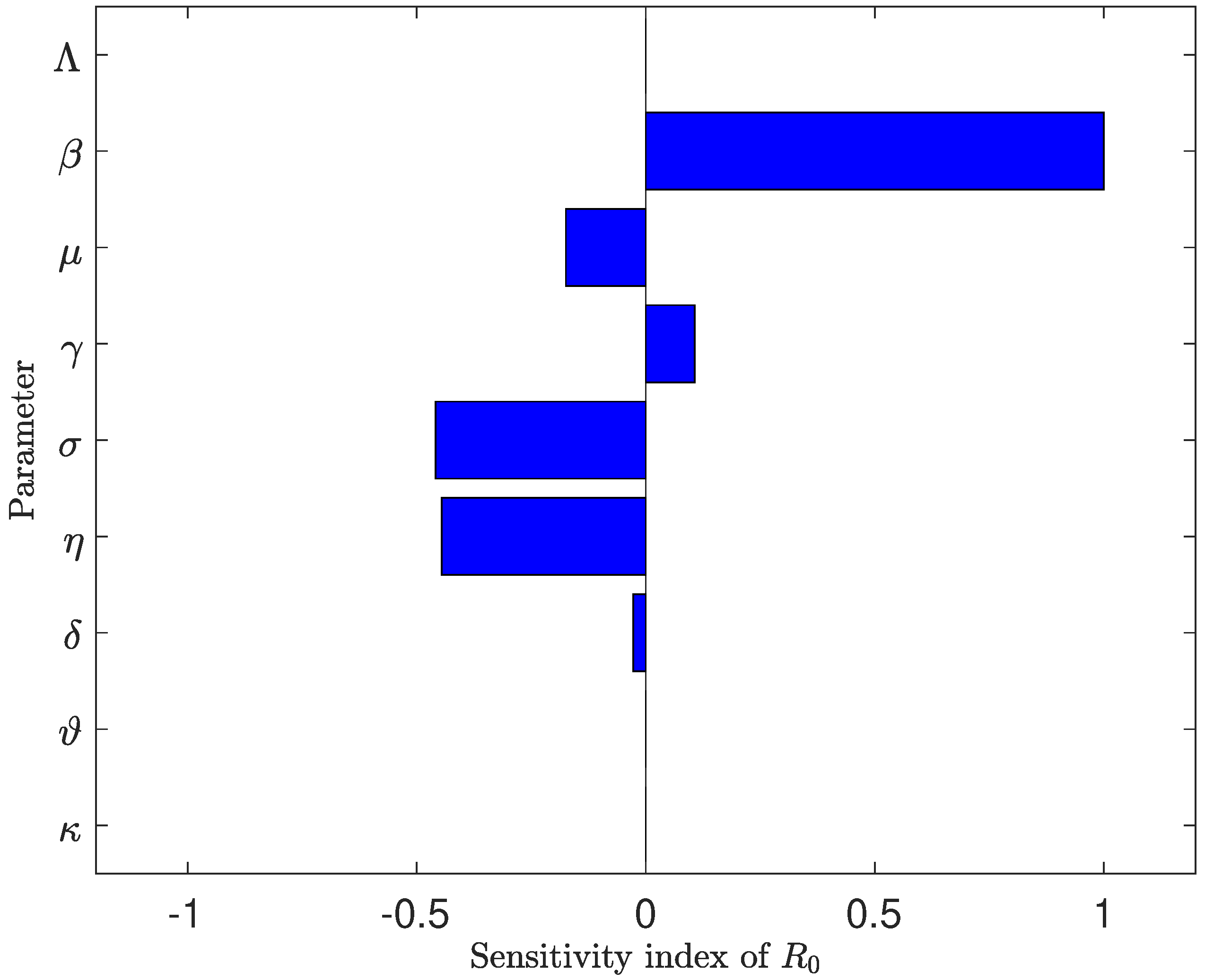
7. Sensitivity Analysis

In this section, we perform sensitivity analysis of basic reproduction number ${\mathcal{R}}_0$. This analysis aims to identify the role of each parameter of model (2) to ${\mathcal{R}}_0$, which is represented by the sensitivity index. The normalized forward sensitivity index of ${\mathcal{R}}_0$ for parameter $\hat{p}$ is formulated by

$$\begin{array}{c}\hfill {\mathcal{I}}_{\hat{p}}^{{\mathcal{R}}_0}=\frac{\hat{p}}{{\mathcal{R}}_0}\times \frac{\partial {\mathcal{R}}_0}{\partial \hat{p}}.\end{array}$$

The greater the absolute value of the index, the more influential the parameter is to ${\mathcal{R}}_0$. The sign of the index shows the enlargement and reduction of ${\mathcal{R}}_0$, that is, a positive sign enlarges ${\mathcal{R}}_0$ while a negative sign reduces ${\mathcal{R}}_0$. We analytically calculate the sensitivity index for each parameter as follows:

$$\begin{array}{ccc}\hfill {\mathcal{I}}_{\Lambda }^{{\mathcal{R}}_0}& =& 0,\hfill \\ \hfill {\mathcal{I}}_{\beta }^{{\mathcal{R}}_0}& =& 1,\hfill \\ \hfill {\mathcal{I}}_{\mu }^{{\mathcal{R}}_0}& =& -\frac{\mu \left((\sigma +\eta +\delta +\mu )+(\gamma +\mu )\right)}{(\gamma +\mu )(\sigma +\eta +\delta +\mu )},\hfill \\ \hfill {\mathcal{I}}_{\gamma }^{{\mathcal{R}}_0}& =& \frac{\mu }{(\gamma +\mu )},\hfill \\ \hfill {\mathcal{I}}_{\sigma }^{{\mathcal{R}}_0}& =& -\frac{\sigma }{(\sigma +\eta +\delta +\mu )},\hfill \\ \hfill {\mathcal{I}}_{\eta }^{{\mathcal{R}}_0}& =& -\frac{\eta }{(\sigma +\eta +\delta +\mu )},\hfill \\ \hfill {\mathcal{I}}_{\delta }^{{\mathcal{R}}_0}& =& -\frac{\delta }{(\sigma +\eta +\delta +\mu )},\hfill \\ \hfill {\mathcal{I}}_{\vartheta }^{{\mathcal{R}}_0}& =& 0,\hfill \\ \hfill {\mathcal{I}}_{\kappa }^{{\mathcal{R}}_0}& =& 0.\hfill \end{array}$$

To display the sensitivity index of ${\mathcal{R}}_0$ for each parameter, we substitute the value of the parameter given in

Table 2. The parameter values of the sensitivity index.

Parameter	Unit	Value	Source
$\Lambda$	$\frac{\mathrm{i}\mathrm{n}\mathrm{d}\mathrm{i}\mathrm{v}\mathrm{i}\mathrm{d}\mathrm{u}\mathrm{a}\mathrm{l}}{\mathrm{d}\mathrm{a}{\mathrm{y}}^{\alpha }}$	$\mathrm{3,270,186}$	[43]
$\beta$	$\frac{1}{\mathrm{d}\mathrm{a}{\mathrm{y}}^{\alpha }}$	$0.29$	[43]
$\mu$	$\frac{1}{\mathrm{d}\mathrm{a}{\mathrm{y}}^{\alpha }}$	$\frac{1}{67.4}$	[43]
$\gamma$	$\frac{1}{\mathrm{d}\mathrm{a}{\mathrm{y}}^{\alpha }}$	$0.1243$	[43]
$\sigma$	$\frac{1}{\mathrm{d}\mathrm{a}{\mathrm{y}}^{\alpha }}$	$0.1$	Assumed
$\eta$	$\frac{1}{\mathrm{d}\mathrm{a}{\mathrm{y}}^{\alpha }}$	$0.09722$	[43]
$\delta$	$\frac{1}{\mathrm{d}\mathrm{a}{\mathrm{y}}^{\alpha }}$	$0.006$	[44]
$\vartheta$	$\frac{1}{\mathrm{d}\mathrm{a}{\mathrm{y}}^{\alpha }}$	$0.1$	Assumed
$\kappa$	$\frac{1}{\mathrm{d}\mathrm{a}{\mathrm{y}}^{\alpha }}$	$0.005$	Assumed

into the index formula for each parameter. The sensitivity indices of ${\mathcal{R}}_0$ are depicted in Figure 2, and the values are given in

Table 3. The value of sensitivity index of ${\mathcal{R}}_0$ with respect to parameter values in Table 2.

Parameter	Value of Sensitivity Index
$\Lambda$	0
$\beta$	1
$\mu$	$-0.1746$
$\gamma$	$0.1066$
$\sigma$	$-0.4585$
$\eta$	$-0.4458$
$\delta$	$-0.0275$
$\vartheta$	0
$\kappa$	0

. It can be seen that parameter $\beta$, $\sigma$, and $\eta$ have important role in reducing ${\mathcal{R}}_0$. However, the sensitivity of $\beta$ is clear because the definition of ${\mathcal{R}}_0$ is very close to disease transmission $\beta$. Thus, we discuss the sensitivity indices of both $\sigma$ and $\eta$, i.e., $-0.4585$ and $-0.4458$, respectively. Since both these indices are negative, the greater the values of $\sigma$ or $\eta$, the smaller ${\mathcal{R}}_0$ is. The results show both parameters $\sigma$ and $\eta$ have an important role in reducing the basic reproduction number and thus have an impact on the stability of the equilibrium point.

8. Numerical Simulation

In this section, we confirm our analytical results by setting the parameter values and implementing a predictor–corrector scheme in [37] to obtain the numerical solution of model (2). The values of the parameters in the first simulation are given by Table 2. Note that the parameter units shown in Table 2 are due to parameter scaling. Therefore, to maintain consistency with the physical dimensions, the units of all model parameters (2) are adjusted to the dimensions $\mathrm{d}\mathrm{a}{\mathrm{y}}^{\alpha }$.

Since the quarantined class has better prevention than the infected one [45], we set the recovery rate to $\vartheta =0.1>\eta$ and the death rate to $\kappa =0.005$. Here, we use (38,000, 2000, 1000, 3000, 50, and 3000) as initial values in the model (2). For these parameters value, we obtain ${\mathcal{R}}_0=1.1881>1$, and thus two equilibrium points exist, namely, the unstable disease-free equilibrium $X^0=(\mathrm{220,410,536.4},$ $0,$ $0,$ $0,$ $0)$ and the globally asymptotically stable endemic equilibrium $X^{\ast }=(\mathrm{184,244,619.17},$ $\mathrm{3,856,537.79},$ $\mathrm{2,198,361.42},$ $\mathrm{1,834,462.79},$ $\mathrm{26,769,323.88})$. These stability properties are verified via our simulation depicted in Figure 3. In Figure 3, there is different behavior for different orders of fractional derivative $\left(\alpha \right)$. It is clear that the smaller the order $\alpha$, the slower the convergence of the solutions is. The peaks are also lower when $\alpha$ is smaller. Furthermore, for the numerical solution of R at $\alpha =0.8$, there is no peak in the time interval $[0,3500]$. However, the curves of the solution for each $\alpha$ have the same behavior and preserve their convergence.

For the second simulation, we execute the model using the parameter values in Table 2, except the quarantine rate is $\sigma =0.2$. For the value of the parameters, we have ${\mathcal{R}}_0=0.81456<1$, and therefore, only one equilibrium exists, that is, a globally asymptotically stable disease-free equilibrium $X^0=(\mathrm{220,410,536.4},$ $0,$ $0,$ $0,$$0)$. This stability equilibrium is confirmed by our numerical simulation, depicted in Figure 4; that is, the disease-free equilibrium $X^0$ is globally asymptotically stable for all orders of fractional derivative $\left(\alpha \right)$. Again, the smaller the order of $\alpha$, the slower the convergence of the solution. Therefore, endemic stability from the first simulation can be prevented by increasing the quarantine rate, which is actually supported by education and lockdown.

For the third simulation, the parameter values listed in Table 2 are used, except the recovery rate of infected individuals is $\eta =0.2$. We have ${\mathcal{R}}_0=0.8075<1$, and therefore, only one equilibrium point exists, that is, a globally asymptotically stable disease-free equilibrium $X^0=(\mathrm{220,410,536.4},$ $0,$ $0,$ $0,$ $0)$. This global asymptotic stability of the disease-free equilibrium is confirmed by our numerical simulation, depicted in Figure 5. We observe that all numerical solutions are convergent to $X^0$. Again, the order $\alpha$ affects the convergence rate of the solution. This simulation is the difference between our paper and those of Zeb et al. [21] and López and Rodó [24], both of whom did not consider the recovery rate of infected class $\eta$. We conclude that the recovery rate of the infected class is important to consider in the COVID-19 epidemic model because it can change the stability of the equilibrium point. Epidemiologically, the recovery rate can be increased by treatment based on Molnupiravir-assisted pharmacotherapy [46].

9. Parameter Estimation

In this section, we estimate the parameter values of model (2) using COVID-19 data from Indonesia. The COVID-19 data are adopted from the daily distribution map of confirmed active COVID-19 cases from the sixth wave, i.e., from 20 October 2022 to 10 January 2023, which is available on the official website of the Indonesian government at Distribution Map of COVID-19. Available online: https://covid19.go.id/peta-sebaran (accessed on 15 January 2023) [47]. The number of confirmed active daily cases corresponds to the infected subpopulations of model (2). The model’s parameter values are then estimated using the least square method, namely by minimizing the squared error between the numerical solution of the infected subpopulations and the data of confirmed active daily cases. To perform this process, we employ a built-in MATLAB function, that is, lsqcurvefit, which is based on the non-linear least square method. The initial value of model (2) is $S\left(0\right)=270\times {10}^6$, $E\left(0\right)$ = 50,000, $I\left(0\right)$ = 18,919, $Q\left(0\right)$ = 17,000, $R\left(0\right)=5\times {10}^6$, $M\left(0\right)$ = 150,000, where $I\left(0\right)$ corresponds to first-day case of the data used. We also set the initial estimates for each parameter, that is, $\Lambda =\frac{270\times {10}^6}{70\times 365}$, $\beta =10$, $\mu =0.00001$, $\gamma =0.2$, $\sigma =0.4$, $\eta =0.9$, $\delta =0.001$, $\vartheta =0.9$, and $\kappa =0.001$. Each parameter value is estimated in the range from 0 to 1, except for recruitment rate $\Lambda$ and disease transmission $\beta$. Ideally, recruitment rate $\Lambda$ is around $\Lambda =\frac{270\times {10}^6}{70\times 365}=\mathrm{10,567}$, where the total population of Indonesia is around $270\times {10}^6$ and the average age of the Indonesian population is around 70 years. Hence, we set $\Lambda$ in the range of 0 to $\mathrm{20,000}$. We assume the estimated value of disease transmission $\beta$ is in the range 0 to 50.

We perform parameter estimation for fractional-order $\alpha =1, 0.97, 0.94, 0.9, 0.87, 0.84, 0.8$. Notice that estimated values of the parameter for $\alpha =1$ correspond to the parameter of the first-order model proposed by Darti et al. [25]. For each value of $\alpha$, model calibration is performed for 63 days of data, i.e., from 20 October 2022, to 21 December 2022, whereas the additional data from 22 December 2022, to 10 January 2023, is used for 20-day forecasting. We compare the calibration and forecasting of both the fractional-order model and the first-order model. To perform this comparison, we determine the root mean square error (RMSE), expressed by

$$\begin{array}{c}\hfill \mathrm{R}\mathrm{M}\mathrm{S}\mathrm{E}=\sqrt{\sum _{k=0}^N{\left(I\left(t_k\right)-I_{\mathrm{d}\mathrm{a}\mathrm{t}\mathrm{a}}\left(t_k\right)\right)}^2},\end{array}$$

where N is the number of data points, $I\left(t_k\right)$ is the numerical solution of the infected compartment of model (2) at $t_k$, and $I_{\mathrm{d}\mathrm{a}\mathrm{t}\mathrm{a}}\left(t_k\right)$ is the data of confirmed daily active cases at $t_k$.

The estimated values of the parameters for different $\alpha$ are shown in

Table 4. Estimated parameter value for different values of derivative order.

Parameter	Derivative Order
	$\mathbf{\alpha }=\mathbf{1}$	$\mathbf{\alpha }=\mathbf{0}.\mathbf{97}$	$\mathbf{\alpha }=\mathbf{0}.\mathbf{94}$	$\mathbf{\alpha }=\mathbf{0}.\mathbf{90}$	$\mathbf{\alpha }=\mathbf{0}.\mathbf{87}$	$\mathbf{\alpha }=\mathbf{0}.\mathbf{84}$	$\mathbf{\alpha }=\mathbf{0}.\mathbf{80}$
$\Lambda$	$20,000$	$1,853.4473$	$0.1936$	$5,259.6532$	$12.6850$	$446.9792$	$11.1194$
$\beta$	$3.2961$	$1.8559$	$2.9466$	$9.5676$	$4.0059$	$4.9821$	$5.7791$
$\mu$	$0.0412$	$0.2193$	$0.3010$	$0.3459$	$0.2764$	$0.3126$	$0.3188$
$\gamma$	1	$0.1081$	$0.1247$	$0.0943$	$0.3604$	$0.3966$	$0.5526$
$\sigma$	1	$0.2452\times {10}^{-4}$	$0.0184$	$0.1745$	$0.5946$	$0.7644$	$0.9999$
$\eta$	1	$0.0930$	$0.1304$	$0.9224$	$0.5185$	$0.5876$	$0.7543$
$\delta$	$0.8812$	$0.1312$	$0.1891$	$0.0042$	$0.4550$	$0.6031$	$0.9764$
$\vartheta$	$0.7624$	$0.0372$	$0.1012$	$0.8045$	$0.0655$	$0.0005$	$0.0004$
$\kappa$	$2.751\times {10}^{-14}$	$0.898\times {10}^{-6}$	$0.3903$	$0.1947$	$0.9111$	$0.9749$	$0.9998$

. Notice that the estimated values of the parameter for each $\alpha$ are different. These cannot be compared between $\alpha$ because different alpha values have different units. The fitted curve for $\alpha =1$, $0.97$, $0.93$, $0.9$, $0.87$, $0.83$, $0.8$ is depicted in Figure 6. The confirmed daily active data used for calibration are marked by red dots, and the data for the 20-day forecasting are marked by blue dots. We discuss the results of calibration and forecasting from the viewpoint of the fitted curve and the obtained RMSE.

For the fitted curve of a first-order model, i.e., when $\alpha =1$, it can be seen that there are large deviations almost everywhere except for around the inflection point and peak point. Fitted curves for the fractional-order model typically have some deviation at the beginning and end of the period. Except at the end of the period, the fitted curves for $\alpha =0.97$ and $\alpha =0.94$ depicted in Figure 6 are good. It should be noted that not all orders $\alpha$ are good for data fitting. For example, the fitted curve for $\alpha =0.9$ appears to have a large deviation from the data used. Thus, the value of $\alpha$ also influences the data fitting performance. Nonetheless, based on the fitted curves, a fractional-order curve is typically better than a first-order curve for calibration and 20-day forecasting. These results show that a fractional-order model has greater flexibility for data fitting, and thus the best-fit curve for the data can be provided.

To confirm the observation of the fitted curves for different values of $\alpha$, we also determine the RMSE for the calibration and 20-day forecasting of confirmed daily active cases given by

Table 5. Root mean square error of the calibration of confirmed COVID-19 cases.

Derivative Order
$\alpha =1$	$\alpha =0.97$	$\alpha =0.94$	$\alpha =0.90$	$\alpha =0.87$	$\alpha =0.84$	$\alpha =0.80$
$2.5880\times {10}^4$	$0.9701\times {10}^4$	$1.5819\times {10}^4$	$3.4915\times {10}^4$	$1.3084\times {10}^4$	$1.4788\times {10}^4$	$1.6319\times {10}^4$

and

Table 6. Root mean square error of 20-day forecasting of confirmed COVID-19 cases.

Derivative Order
$\alpha =1$	$\alpha =0.97$	$\alpha =0.94$	$\alpha =0.90$	$\alpha =0.87$	$\alpha =0.84$	$\alpha =0.80$
$4.1023\times {10}^4$	$1.7944\times {10}^4$	$2.7407\times {10}^4$	$7.4194\times {10}^4$	$1.8617\times {10}^4$	$2.2247\times {10}^4$	$2.7200\times {10}^4$

, respectively. It can be seen that the RMSE of calibration for the fractional-order model is smaller than the first-order model, except for $\alpha =0.9$. The smallest RMSE of calibration occurs when fractional order $\alpha =0.97$, where, in this case, the fractional-order model has a RMSE that is $2.7$ times smaller than the first-order model. These results verify that a fractional-order model generally performs better than a first-order model in calibrating the COVID-19 data. Similarly, the RMSE of the 20-day forecasting for the fractional-order model is also smaller than the first-order model, except for $\alpha =0.9$. Again, a fractional-order model generally provides better 20-day forecasts than a first-order model, especially the fractional-order model with $\alpha =0.97$, which has an RMSE that is $2.3$ times smaller than the first-order model. Finally, we can say a fractional-order model has better accuracy and flexibility than a first-order model when implemented using confirmed daily active cases of COVID-19 in Indonesia. This also confirms the statement of Alrabaiah et al. [29] that a fractional-order model is more flexible than a first-order model.

10. Conclusions

We construct a fractional-order COVID-19 epidemic model with quarantine and standard incidence rate using the Caputo fractional-order derivative. We modify earlier models by simultaneously considering the recovery rate and quarantine rate of infected individuals. We also consider the standard incidence rate in the model. We have proven the existence, uniqueness, non-negativity, and boundedness of the solution. The model has two equilibrium points, i.e., a disease-free equilibrium and an endemic equilibrium. We obtain the basic reproduction number (${\mathcal{R}}_0$) by implementing the spectral radius of the next-generation matrix. The disease-free equilibrium always exists and is locally and globally asymptotically stable only if ${\mathcal{R}}_0<1$. In contrast, the endemic equilibrium exists and is globally asymptotically stable if ${\mathcal{R}}_0>1$. The stability properties of the equilibrium points are confirmed by numerical simulation. From the numerical simulation, we can see that the smaller the order of the derivative, the slower the convergence of the solution of the model and vice versa. In addition, we conclude that both the recovery rate and quarantine rate of the infected class have an important role in reducing ${\mathcal{R}}_0$, as well as for the stability of the equilibrium point. Based on parameter estimation results, a fractional-order model typically performs better than a first-order model for both calibrating and forecasting confirmed cases of COVID-19 in Indonesia. In our case, the fractional-order model with $\alpha =0.97$ has an RMSE that is twice as small as the first-order model for both the calibration and forecasting of confirmed COVID-19 cases.