
Bivariate Discrete Odd Generalized Exponential Generator of Distributions for Count Data: Copula Technique, Mathematical Theory, and Applications
 ,
,
Abstract
:1. Introduction
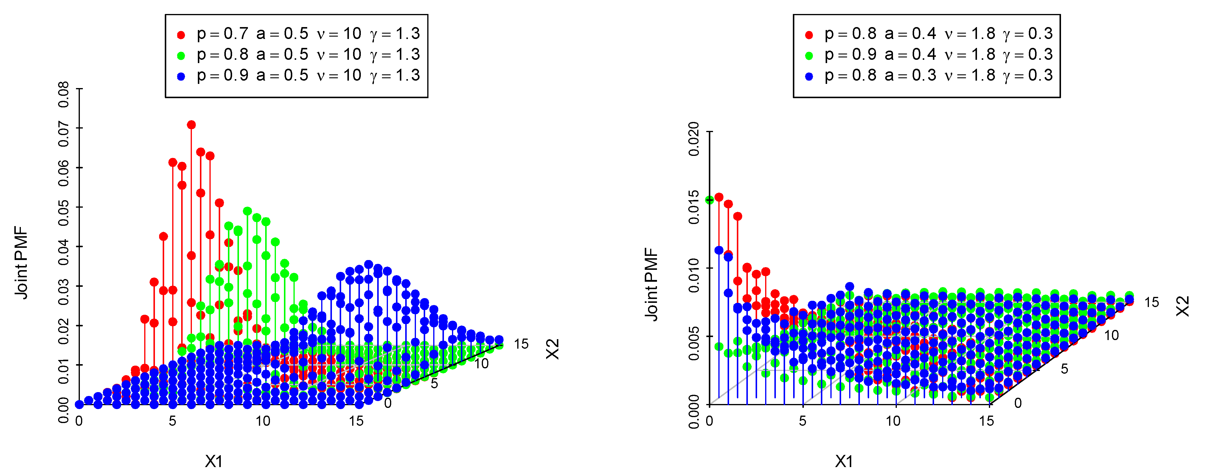
2. The BDOGE-G Class
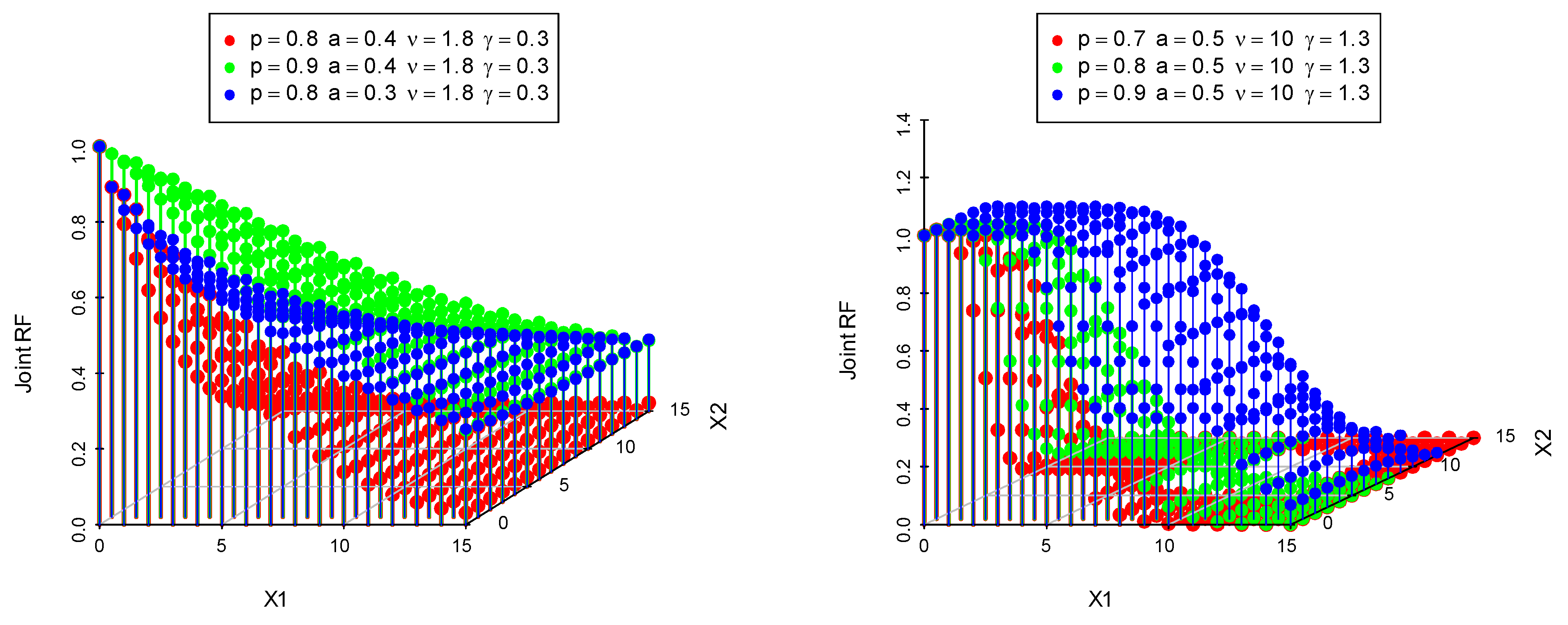
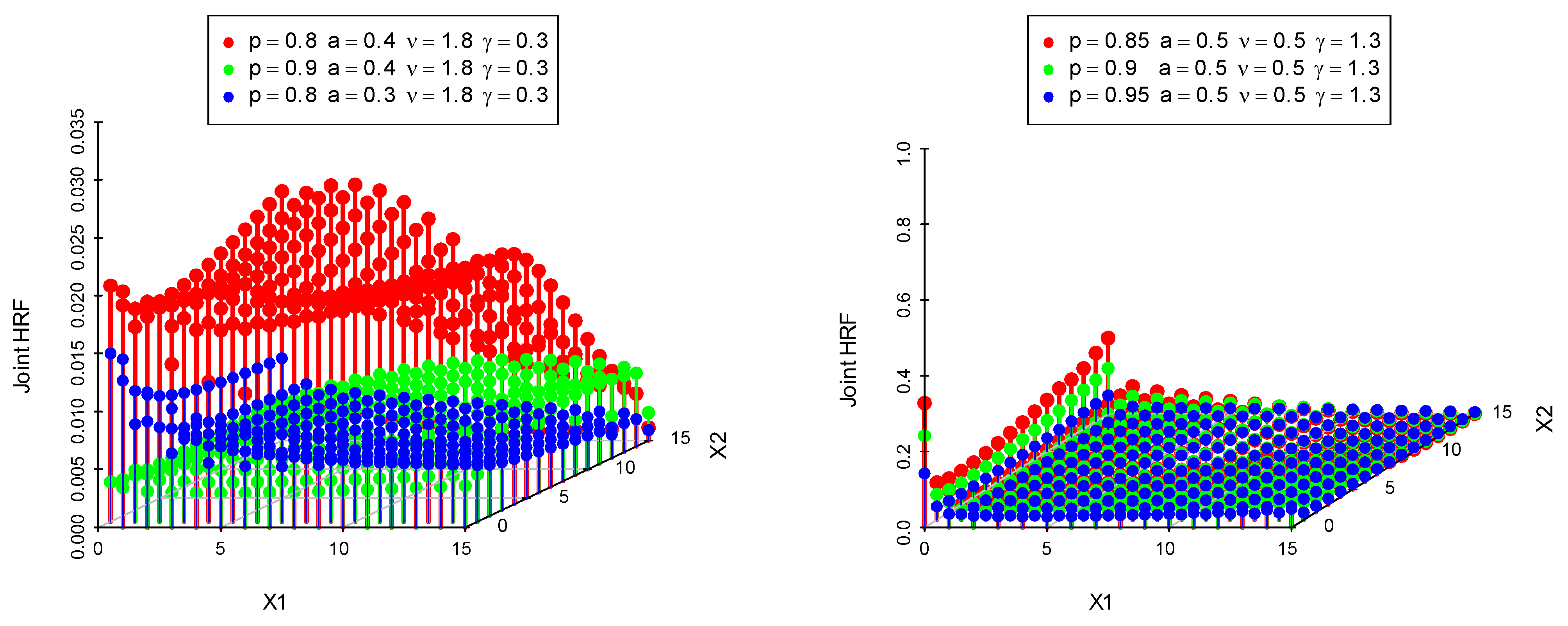
3. Distributional Properties
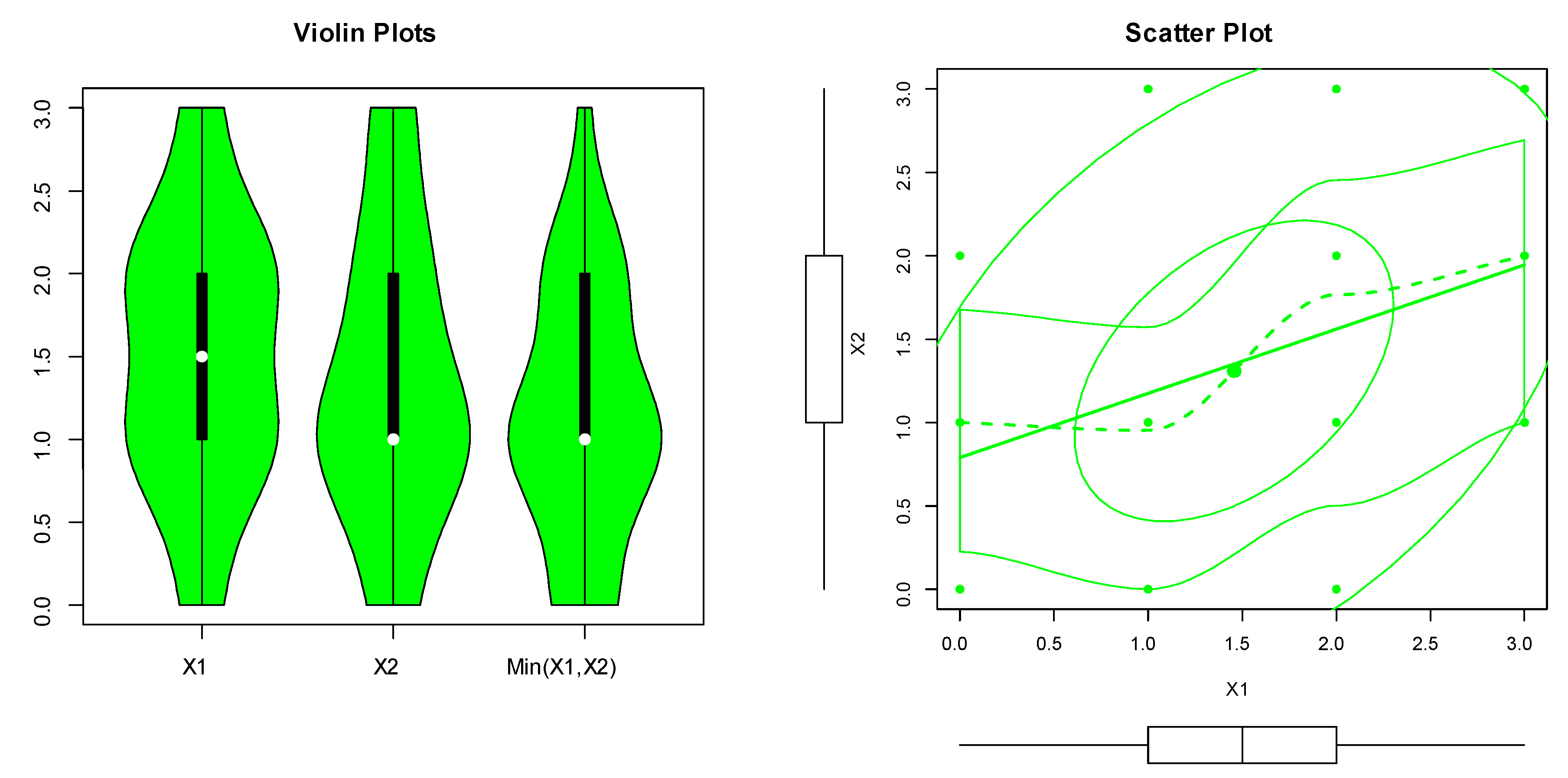
3.1. Median Correlation Coefficient
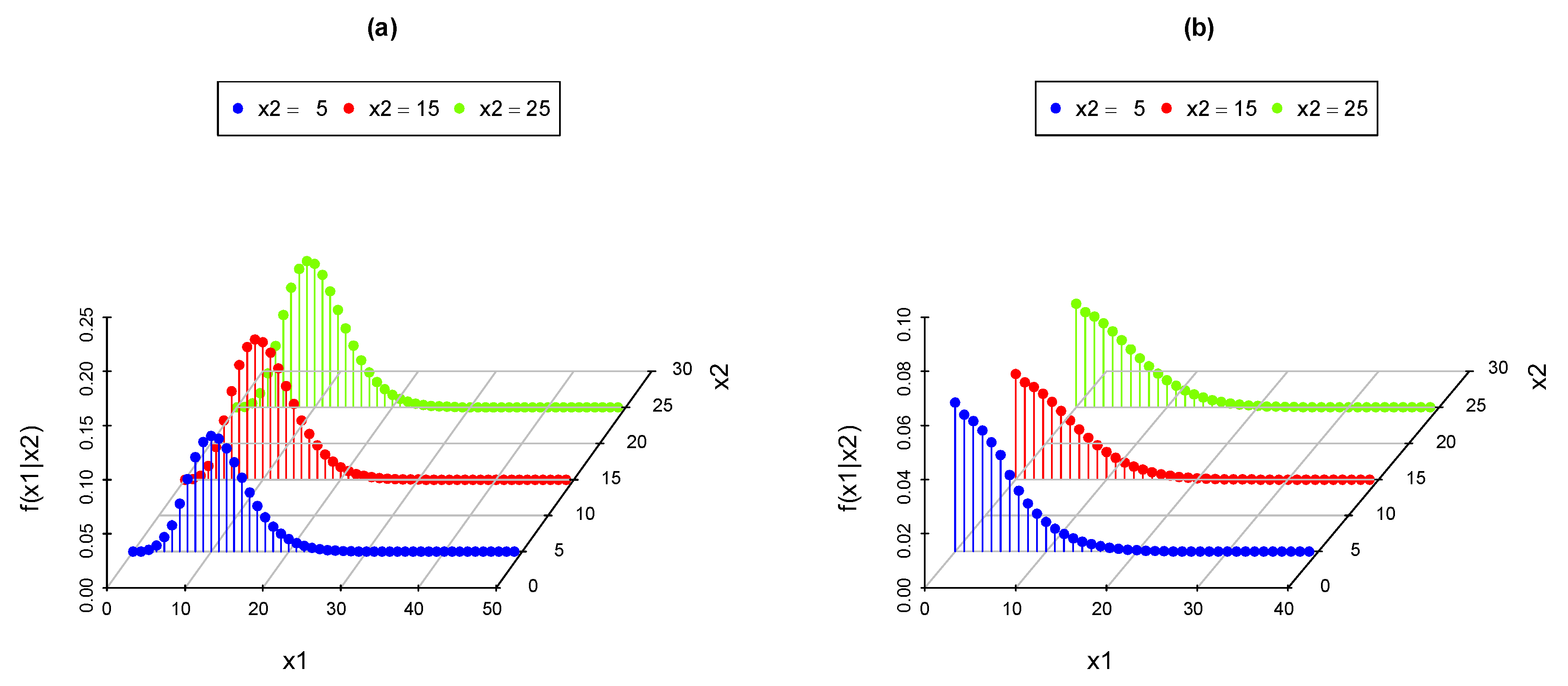
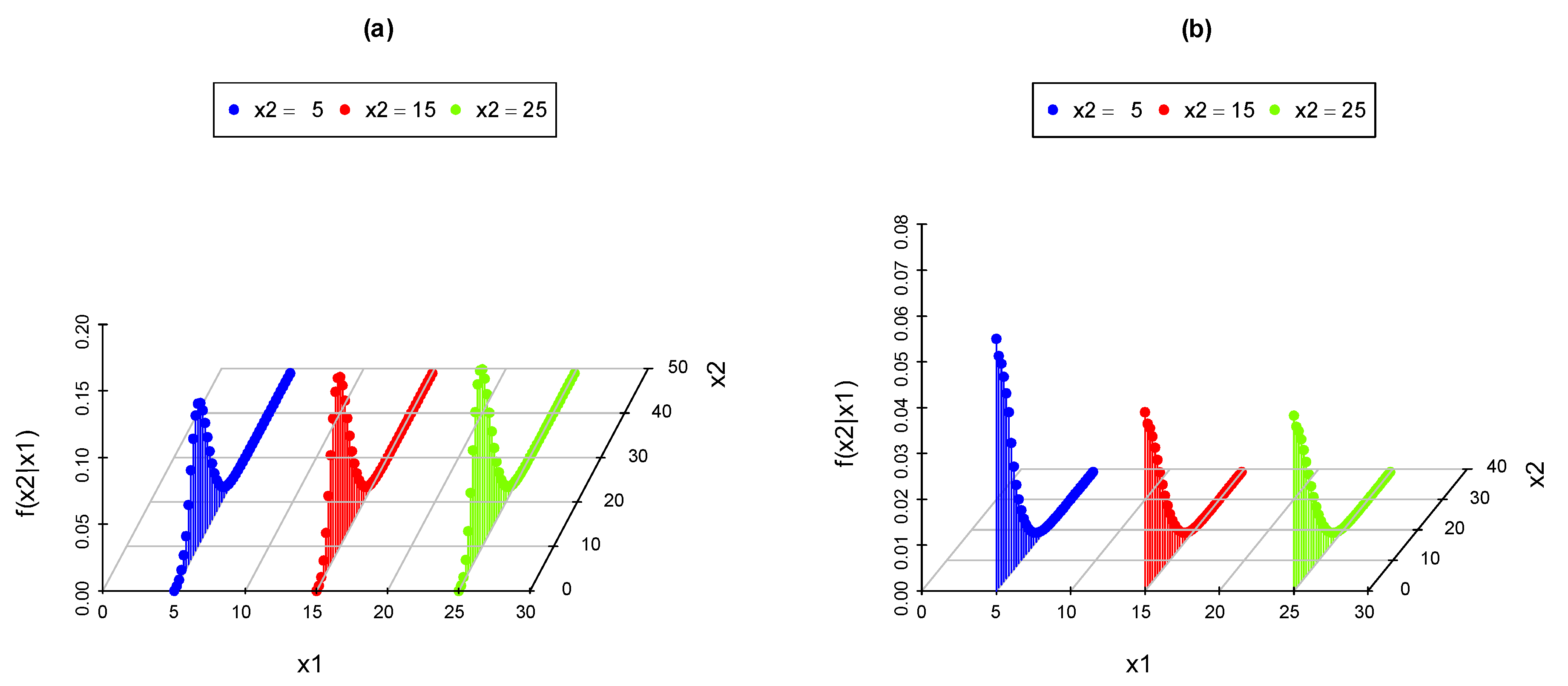
3.2. The Conditional CDF of Given ()
3.3. The Conditional Expectation of Given
4. The BDsOGE-Weibull (BDsOGEW) Distribution
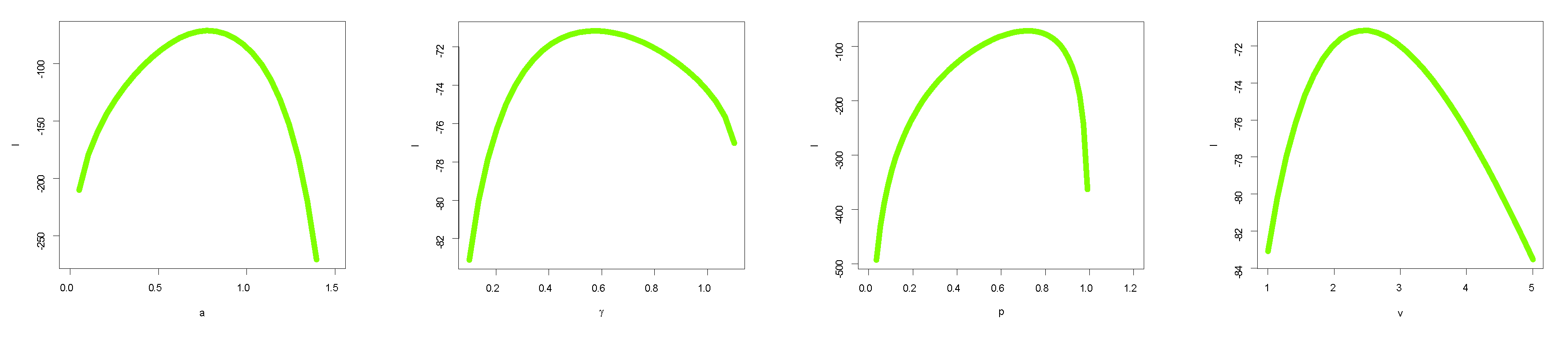
5. Point and Interval Estimations
5.1. Maximum Likelihood Estimation (MLE)
5.2. Asymptotic Confidence Intervals
6. Simulation: Estimators Performance
- Scheme I: (∀= == = | = 20, = 50, = 150, = 300, = 500, = 700);
- Scheme II: (∀= == = | = 20, = 50, = 150, = 300, = 500, = 700);
- Scheme III: (∀= == = | = 20, = 50, = 150, = 300, = 500, = 700)
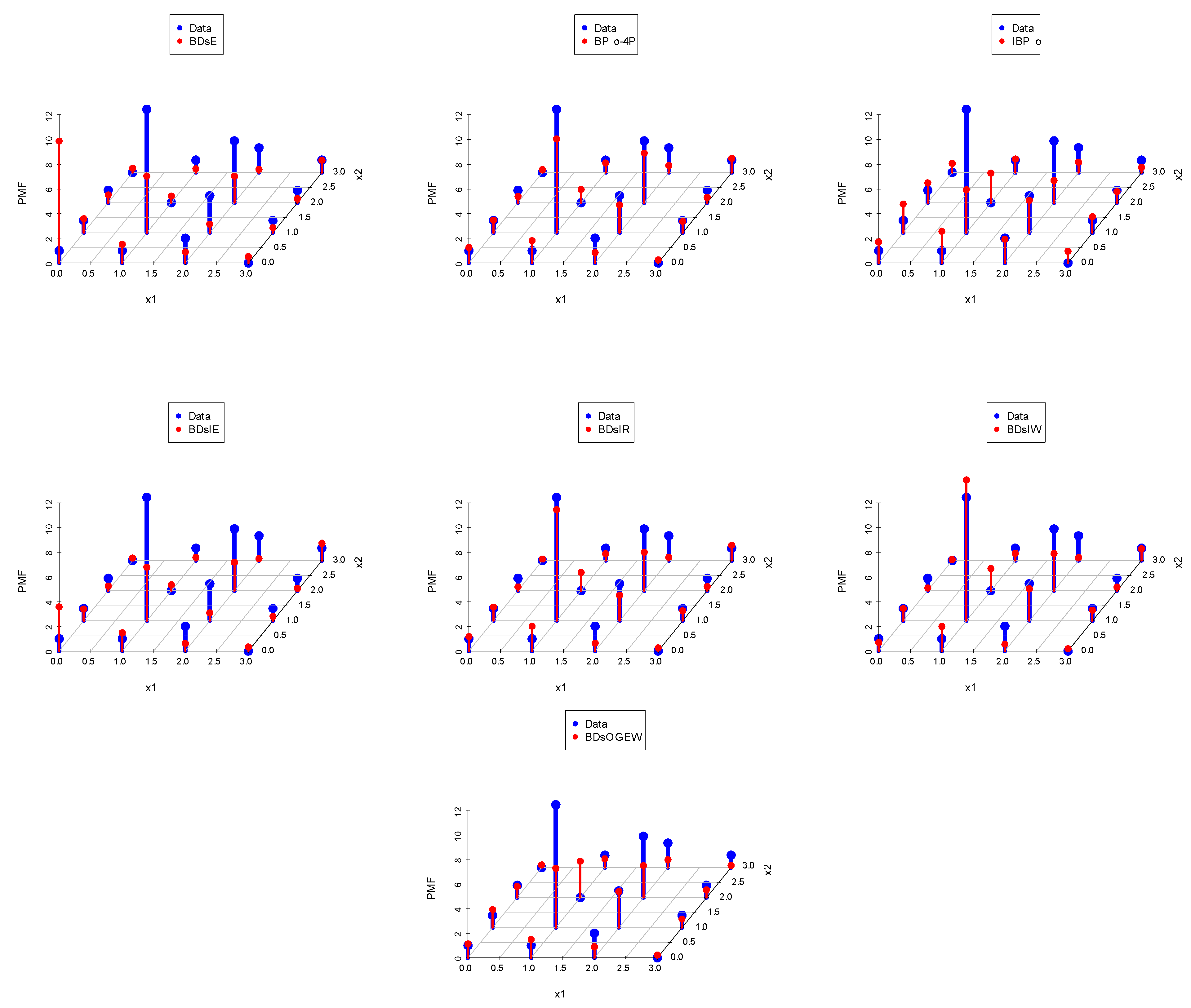
7. Data Analysis
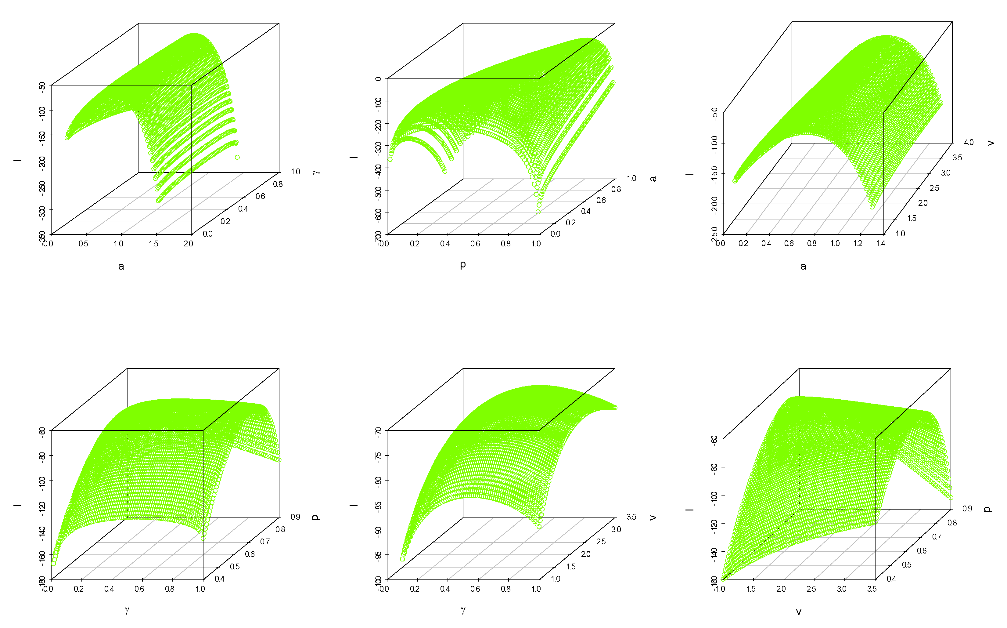
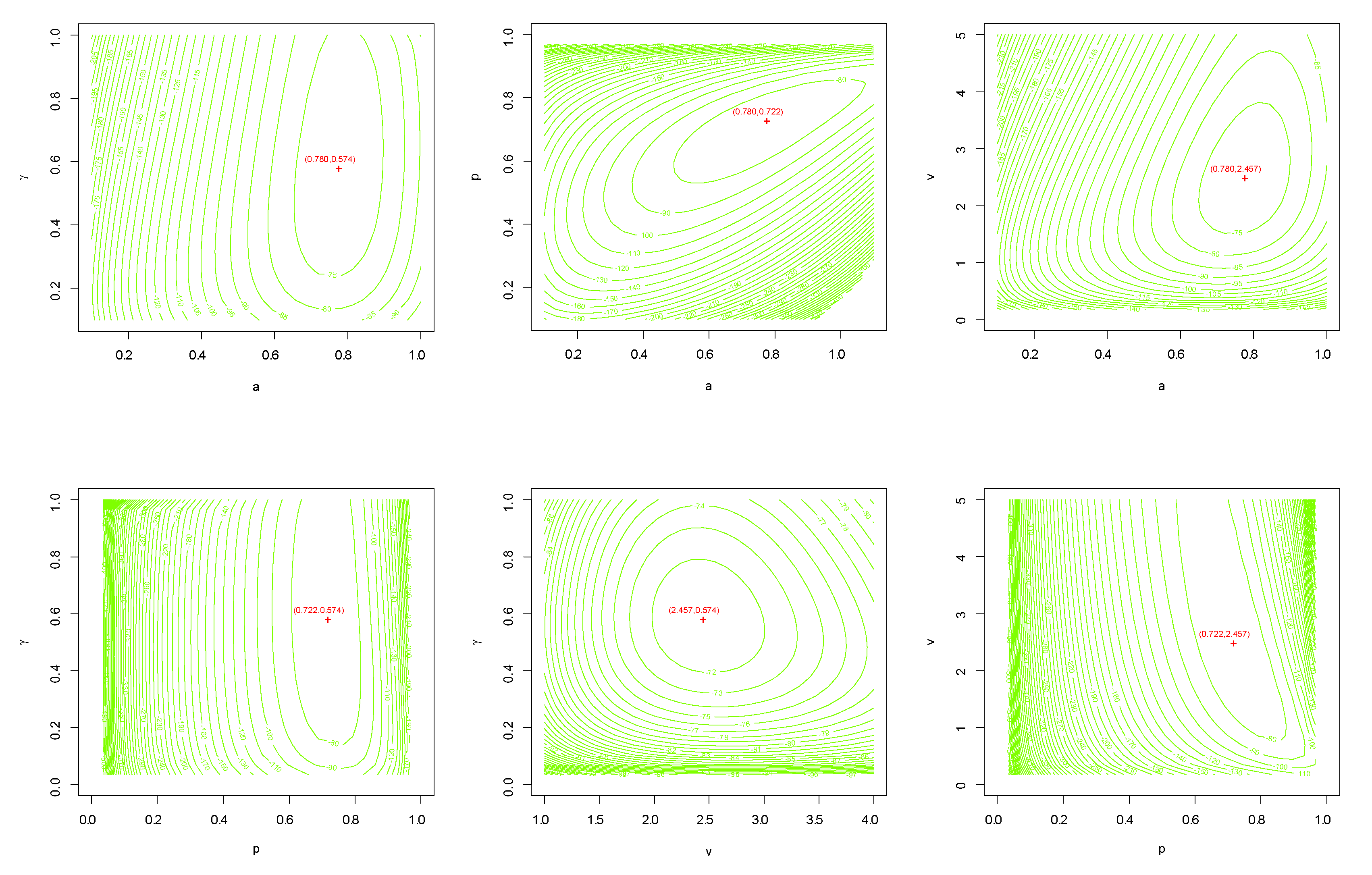
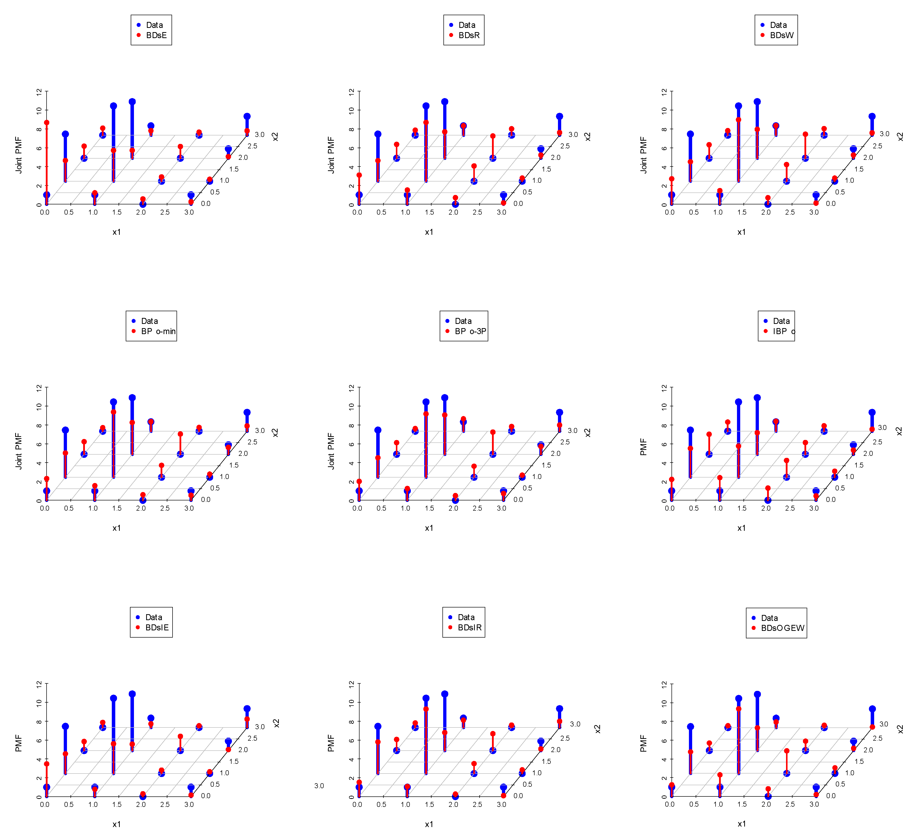
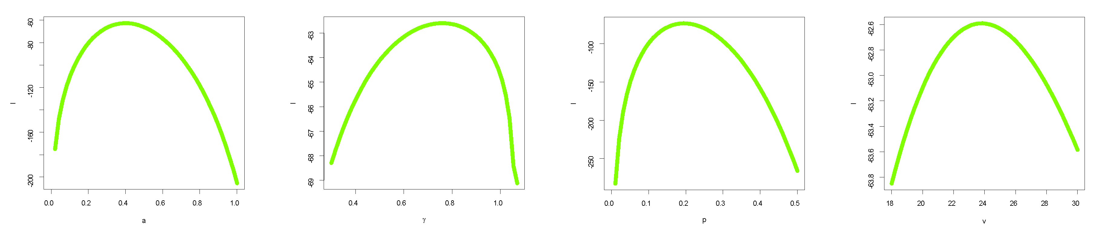
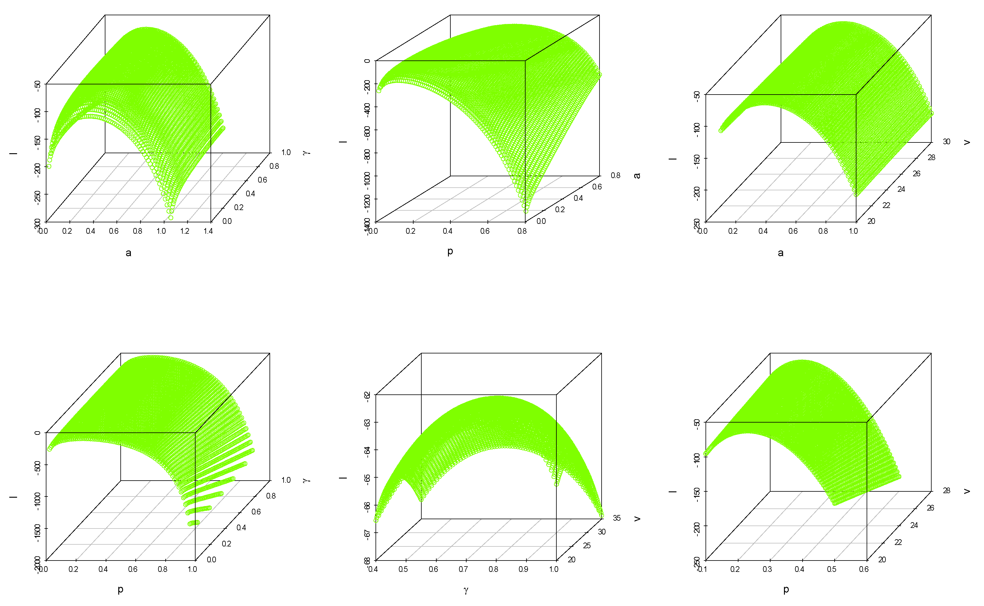
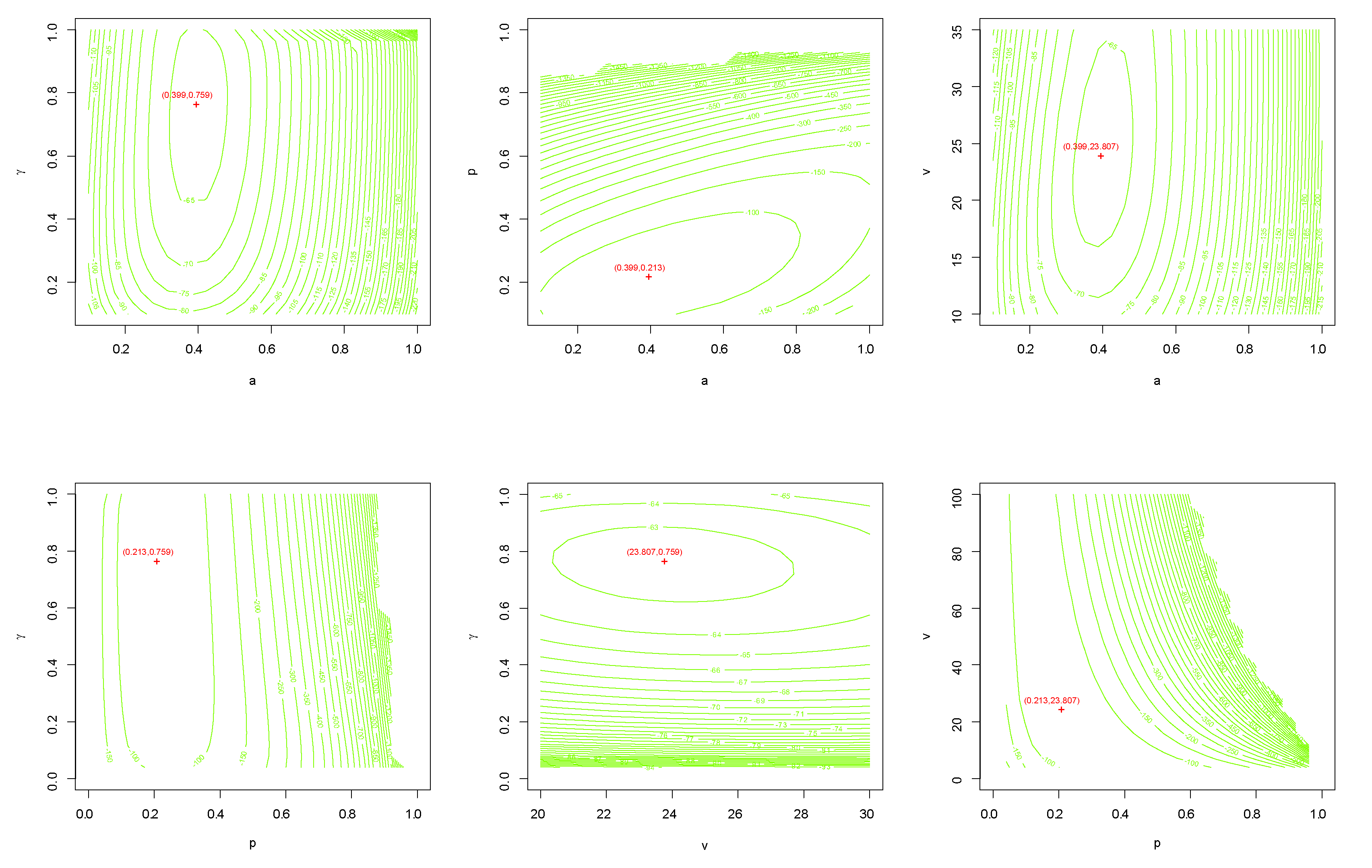
7.1. Data Set I: Nasal Drainage Severity Score
7.2. Data Set II: Football Score
8. Concluding Remarks and Future Work
Author Contributions
Funding
Data Availability Statement
Acknowledgments
Conflicts of Interest
Appendix A
- The PMF of the BDsOGE-G
- Estimation code for real data
References
- Alzaatreh, A.; Lee, C.; Famoye, F. A new method for generating families of continuous distributions. Metron 2013, 71, 63–79. [Google Scholar] [CrossRef]
- Tahir, M.H.; Cordeiro, G.M.; Alizadeh, M.; Mansoor, M.; Zubair, M.; Hamedani, G.G. The odd generalized exponential family of distributions with applications. J. Stat. Appl. 2015, 2, 1. [Google Scholar] [CrossRef]
- Silva, G.F.S.; Percontini, A.; de Brito, E.; Ramos, M.W.; Venâncio, R.; Cordeiro, G.M. The odd Lindley-G family of distributions. Austrian J. Stat. 2017, 46, 65–87. [Google Scholar] [CrossRef]
- Alizadeh, M.; Ghosh, I.; Yousof, H.M.; Rasekhi, M.; Hamedani, G.G. The generalized odd generalized exponential family of distributions: Properties, characterizations and applications. J. Data Sci. 2017, 15, 443–465. [Google Scholar] [CrossRef]
- Korkmaz, M.C.; Yousof, H.M.; Hamedani, G.G. The exponential Lindley odd log-logistic-G family: Properties, characterizations and applications. J. Stat. Theory Appl. 2018, 17, 554–571. [Google Scholar] [CrossRef]
- Djibrila, S. The generalized odd inverted exponential-G family of distributions: Properties and applications. Eurasian Bull. Math. 2019, 2, 86–110. [Google Scholar]
- Reyad, H.; Othman, S.; Ul Haq, M.A. The transmuted generalized odd generalized exponential-G family of distributions: Theory and applications. J. Data Sci. 2019, 17, 279–300. [Google Scholar] [CrossRef]
- Alizadeh, M.; Afify, A.Z.; Eliwa, M.S.; Ali, S. The odd log-logistic Lindley-G family of distributions: Properties, Bayesian and non-Bayesian estimation with applications. Comput. Stat. 2020, 35, 281–308. [Google Scholar] [CrossRef]
- Balakrishnan, N.; Lai, C.D. Continuous Bivariate Distributions, 2nd ed.; Wiley: New York, NY, USA, 2009; Volume 1. [Google Scholar]
- Johnson, M.E.; Tenenbein, A. A bivariate distribution family with specified marginals. J. Am. Assoc. 1981, 76, 198–201. [Google Scholar] [CrossRef]
- Quesada-Molina, J.J.; Rodrguez-Lallena, J.A. Bivariate copulas with quadratic sections. Journaltitle Nonparametr. Stat. 1995, 5, 323–337. [Google Scholar] [CrossRef]
- Fang, K.T.; Fang, H.B.; Rosen, D.V. A family of bivariate distributions with non-elliptical contours. Commun.-Stat.-Theory Methods 2000, 29, 1885–1898. [Google Scholar] [CrossRef]
- Durante, F. A new family of symmetric bivariate copulas. Comptes Rendus Math. 2007, 344, 195–198. [Google Scholar] [CrossRef]
- Kundu, D.; Gupta, R.D. A class of bivariate models with proportional reversed hazard marginals. Sankhya B 2010, 72, 236–253. [Google Scholar] [CrossRef]
- Sarabia, J.M.; Prieto, F.; Jorda, V. Bivariate beta-generated distributions with applications to well-being data. J. Stat. Distrib. Appl. 2014, 1, 15. [Google Scholar] [CrossRef]
- Roozegar, R.; Jafari, A.A. On bivariate exponentiated extended Weibull family of distributions. arXiv 2015, arXiv:1507.07535. [Google Scholar] [CrossRef]
- Eliwa, M.S.; Alhussain, Z.A.; Ahmed, E.A.; Salah, M.M.; Ahmed, H.H.; El-Morshedy, M. Bivariate Gompertz generator of distributions: Statistical properties and estimation with application to model football data. J. Natl. Sci. Found. Sri Lanka 2020, 48. [Google Scholar] [CrossRef]
- Lee, H.; Cha, J.H. On two general classes of discrete bivariate distributions. Am. Stat. 2015, 69, 221–230. [Google Scholar] [CrossRef]
- Kundu, D.; Nekoukhou, V. Univariate and bivariate geometric discrete generalized exponential distributions. J. Stat. Theory Pract. 2018, 12, 595–614. [Google Scholar] [CrossRef]
- El-Morshedy, M.; Eliwa, M.S.; El-Gohary, A.; Khalil, A.A. Bivariate exponentiated discrete Weibull distribution: Statistical properties, estimation, simulation and applications. Math. Sci. 2020, 14, 29–42. [Google Scholar] [CrossRef]
- Nekoukhou, V.; Khalifeh, A.; Bidram, H. A bivariate discrete inverse resilience family of distributions with resilience marginals. J. Appl. Stat. 2020, 48, 1071–1091. [Google Scholar] [CrossRef] [PubMed]
- De Oliveira, R.P.; Achcar, J.A. A new flexible bivariate discrete Rayleigh distribution generated by the Marshall-Olkin family. Model Assist. Stat. Appl. 2020, 15, 19–34. [Google Scholar] [CrossRef]
- Kobus, M.; Kurek, R. Copula-based measurement of interdependence for discrete distributions. J. Math. 2018, 79, 27–39. [Google Scholar] [CrossRef]
- Najarzadegan, H.; Alamatsaz, M.H.; Kazemi, I. Discrete bivariate distributions generated by copulas: Dbeew distribution. J. Stat. Theory Pract. 2019, 13, 1–30. [Google Scholar] [CrossRef]
- Yamaguchi, Y.; Maruo, K. Bivariate beta-binomial model using Gaussian copula for bivariate meta-analysis of two binary outcomes with low incidence. Jpn. J. Stat. Data Sci. 2019, 2, 347–373. [Google Scholar] [CrossRef]
- Emura, T.; Matsui, S.; Rondeau, V. Survival Analysis with Correlated Endpoints: Joint Frailty-Copula Models; Springer: Berlin/Heidelberg, Germany, 2019. [Google Scholar]
- Cuadras, C.M.; Augé, J. A continuous general multivariate distribution and its properties. Commun.-Stat.-Theory Methods 1981, 10, 339–353. [Google Scholar] [CrossRef]
- Casella, G.; Berger, R.L. Statistical Inference; Duxbury Press: Pacific Grove, CA, USA, 2002. [Google Scholar]
- Pfeiffer, P.E. Conditional Independence in Applied Probability; Springer Science & Business Media: Berlin/Heidelberg, Germany, 2013. [Google Scholar]
- Davis, C.S. Statistical Methods for the Analysis of Repeated Measures Data; Springer: New York, NY, USA, 2002. [Google Scholar]


| p | p | ||||||||
| Bias | |||||||||
| MSE | |||||||||
| CP | |||||||||
| CI | |||||||||
| CI | |||||||||
| p | p | ||||||||
| Bias | |||||||||
| MSE | |||||||||
| CP | |||||||||
| CI | |||||||||
| CI | |||||||||
| p | p | ||||||||
| Bias | |||||||||
| MSE | |||||||||
| CP | |||||||||
| CI | |||||||||
| CI | |||||||||
| p | p | ||||||||
| Bias | |||||||||
| MSE | |||||||||
| CP | |||||||||
| CI | |||||||||
| CI | |||||||||
| p | p | ||||||||
| Bias | |||||||||
| MSE | |||||||||
| CP | |||||||||
| CI | |||||||||
| CI | |||||||||
| p | p | ||||||||
| Bias | |||||||||
| MSE | |||||||||
| CP | |||||||||
| CI | |||||||||
| CI | |||||||||
| p | p | ||||||||
| Bias | |||||||||
| MSE | |||||||||
| CP | |||||||||
| CI | |||||||||
| CI | |||||||||
| p | p | ||||||||
| Bias | |||||||||
| MSE | |||||||||
| CP | |||||||||
| CI | |||||||||
| CI | |||||||||
| p | p | ||||||||
| Bias | |||||||||
| MSE | |||||||||
| CP | |||||||||
| CI | |||||||||
| CI | |||||||||
| Model | MLEs | AIC | HQIC | |
|---|---|---|---|---|
| BDsE | ||||
| BPo-4P | ||||
| IBPo | ||||
| BDsIE | ||||
| BDsIR | ||||
| BDsIW | ||||
| BDsOGEW |
| Model | MLEs | AIC | HQIC | |
|---|---|---|---|---|
| BDsE | ||||
| BDsR | ||||
| BDsW | ||||
| BPo | ||||
| BPo-3P | ||||
| IBPo | ||||
| BDsIE | ||||
| BDsIR | ||||
| BDsOGEW |
Disclaimer/Publisher’s Note: The statements, opinions and data contained in all publications are solely those of the individual author(s) and contributor(s) and not of MDPI and/or the editor(s). MDPI and/or the editor(s) disclaim responsibility for any injury to people or property resulting from any ideas, methods, instructions or products referred to in the content. |
© 2023 by the authors. Licensee MDPI, Basel, Switzerland. This article is an open access article distributed under the terms and conditions of the Creative Commons Attribution (CC BY) license (https://creativecommons.org/licenses/by/4.0/).
Share and Cite
Al-Essa, L.A.; Eliwa, M.S.; Shahen, H.S.; Khalil, A.A.; Alqifari, H.N.; El-Morshedy, M. Bivariate Discrete Odd Generalized Exponential Generator of Distributions for Count Data: Copula Technique, Mathematical Theory, and Applications. Axioms 2023, 12, 534. https://doi.org/10.3390/axioms12060534
Al-Essa LA, Eliwa MS, Shahen HS, Khalil AA, Alqifari HN, El-Morshedy M. Bivariate Discrete Odd Generalized Exponential Generator of Distributions for Count Data: Copula Technique, Mathematical Theory, and Applications. Axioms. 2023; 12(6):534. https://doi.org/10.3390/axioms12060534
Chicago/Turabian StyleAl-Essa, Laila A., Mohamed S. Eliwa, Hend S. Shahen, Amal A. Khalil, Hana N. Alqifari, and Mahmoud El-Morshedy. 2023. "Bivariate Discrete Odd Generalized Exponential Generator of Distributions for Count Data: Copula Technique, Mathematical Theory, and Applications" Axioms 12, no. 6: 534. https://doi.org/10.3390/axioms12060534