

Practical Consequences of Quality Views in Assessing Software Quality


Abstract
:1. Introduction
- Internal quality view:
- Set of quality properties of the source code and documentation that are deemed to influence the behaviour and use of the software.
- External quality view:
- Set of quality properties that determine how the software product behaves while it operates. These properties are usually measured when the software product is operational and is being tested.
- Quality in use view:
- Set of quality properties that determine how the user perceives software product quality, and how far the goals for which the software is used can be achieved.
2. Materials and Methods
3. Results
3.1. Model Simplification
3.1.1. Modelling Steps
3.1.2. Checking the Constructed Model
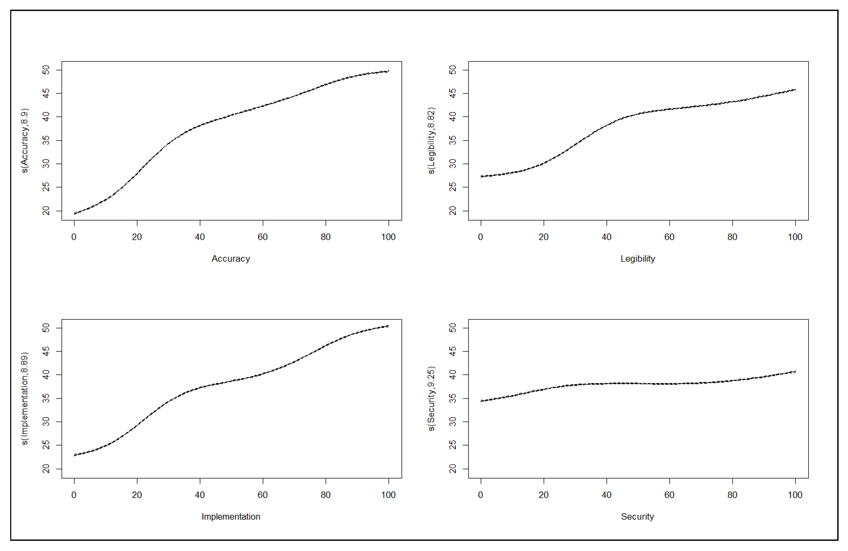
- Since the value of the simplified model was , it can be stated that 77.5% of the variability of the output variable of the fuzzy model was explained by the variability of the output variable of the GAM model, which can be interpreted as an acceptable fit for the simplified model. Table 3 presents the smooth terms with their effective degrees of freedom and the performed F-test statistics with the corresponding p-values. All smooth terms are statistically significant. Thus, the identified smooth functions contribute significantly to the output variable.
- Considering the research settings of [67] and the data generation from the fuzzy model described above, it is unlikely that the inputs have parallel curves, although this was examined.
- Linear correlation:
- Table 4 provides the Pearson correlation between each pair of variables, and it is obvious that there is a lack of linear correlation between the pairs of input variables. The strongest linear correlations between the input variables and the output variable are for the variables Accuracy and Implementation, while the linear correlation of the input variable Security with the output variable is nearly negligible, which conforms with Figure 1.
- Concurvity:
- GAM concurvity measures the extent up to which a “smooth term in a model can be approximated by one or more of the other smooth terms in the model” (concurvity measures: https://stat.ethz.ch/R-manual/R-devel/library/mgcv/html/concurvity.html, accessed on 20 April 2023). GAM concurvity is measured in the range , with no problem identified with a 0 value, while total concurvity is achieved when value 1 is obtained. Table 5 shows the concurvity values. Considering the worst case, all values lie in the vicinity of zero, indicating that the input variables do not have a non-linear relationship.
- The smooth functions are constructed from basis functions to model the patterns found in the data set. If the number of basis functions is too low, then some patterns are missed in the data. The p-values in Table 6 show no significance. (The mgcv R library offers a function to perform this computation, as demonstrated in Appendix A. This check resulted in increasing the number of basis functions for the input variable Security to avoid a significant p-value.) This means that the number of basis functions is appropriate to cover the existing patterns in the data set.
3.1.3. Conclusions of Model Simplification
3.2. Case Studies
3.2.1. Case Study 1: Validity of Statements Based on a Given Software Product Quality Model
- Background:
- Based on the SQALE model, SonarQube [66] is a widespread tool for quality measurement and assessment, with easy-to-use integration into the project life-cycle [2,3,30]. Technical debt is one major element of the SQALE definition [30], which refers to any non-conformance of coding standards described in the form of a rule set. Each identified non-conformance is also associated with a remediation cost in time units to improve the given defect. The identified defects can also be associated with non-remediation costs, which describe the impact of the defect on the system as a whole. However, the estimation of non-remediation costs is vague and error-prone; therefore, the identified defects are usually classified based on criticality from blocker to information on an ordinal scale.Company A decides to introduce measures to apply SonarQube in each software development project and the company defines its own rule sets to identify technical debts using the tool. A project team at company A has already integrated SonarQube [66] into their project but they would like to know to what extent the tool is able to measure software quality as a whole and to what extent the team can rely on the measurement results. This is also an extremely important question when transferring projects for maintenance to external service providers, where software quality can have a direct impact on the financial negotiations.
- Step 1:
- Participants in the development project check the documentation of SonarQube and they find that SQALE is the underlying software product quality model.
- Step 2:
- After successfully identifying the software product quality model, the project team looks up SQALE in Table 2 and they find that SQALE is able to measure and assess only one of the three different manifestations of software product quality, which is a fraction of the whole.
- Result:
- The project team draws the conclusion that SonarQube can measure and assess how the source code is written; moreover, the measurements are performed in a consistent and precise manner. However, SonarQube cannot measure and assess (i) the architecture, (ii) how the software behaves while it runs, and (iii) whether the end user is satisfied with the product. Consequently, SonarQube’s results might be valid for source code quality, depending on the rule set applied during the quality measurement, but these results cannot be considered valid for software product quality in general. Measuring and assessing software product quality as a whole requires the measurement and assessment of all three quality views: internal, external, and quality in use. Thus, the SonarQube results need to be supplemented with the measurement and assessment of the operational behaviour of the software and with the measurement and assessment of the end user feedback to be able to judge software quality as a whole.
3.2.2. Case Study 2a: Selecting a Quality Model for Measurement and Assessment, and Tailoring It to Specific Project Needs
- Background:
- This case study shows how a software product quality model can be selected and the quality requirements refined with regard to a certain project. Eeles’s checklist [48] can be of assistance to collect non-functional and architectural requirements. The stakeholders formulate the following quality guidelines: (1) source code quality must be measured and assessed, (2) the quality of the operational software must be measured and assessed, and (3) the perception of the end user regarding the software must also be measured, assessed, and reported after each defined milestone in the project’s life-cycle.
- Step 1:
- Considering the stakeholders’ guidelines, members of the project team recognise that the selected software product quality model needs the capability to measure all three distinct quality views: internal, external, and quality in use. Thus, as per Table 2, the following models are eligible: ISO/IEC 25010 [10], ISO/IEC 9126 [19], Quamoco [31,32,33,34], ADEQUATE [42,43], GEQUAMO [51], GQM [57], SQUID [62].
- Step 2:
- The project team needs to select a software product quality model for measurement and assessment. The GQM [57] and SQUID [62] approaches would require the creation of a quality model individually, which the project team would avoid. The project team wishes to use a widespread quality model with constant research interest and industrial use cases, which narrows down the set of eligible quality models to ISO/IEC 25010 [10] and ISO/IEC 9126 [19]. From these two models, the project team selects ISO/IEC 25010 [10] because it supersedes the predecessor standard ISO/IEC 9126 [19].
- Step 3:
- After familiarising themselves with the extensive definition of the ISO/IEC 25010 [10] standard, the project team considers how to measure and assess software product quality for each distinct quality view. This provides the project team with an important insight: they need to set up static code analysers individually and interpret their results for the selected high-level quality properties that they use from the standard. Kim and Lee published a similar study in [50]. However, the effort required for the whole setup motivates the team to look for alternatives. They come to the conclusion that they will use a different quality model for the measurement and assessment of the internal quality view, which offers automation potential and requires less effort while integrating into the development pipeline. Consulting Table 2 and the study in [2], they decide to use the SQALE model [30], which offers easy integration into the software life-cycle through tool implementation including SonarQube [66]; moreover, they make the decision to accept the default rule set for their target programming language.
- Step 4:
- The project team outlines the measurement and assessment for the external and quality in use views, based on the ISO/IEC 25010 standard [10], which makes it possible to investigate the operational software and the feedback of the end user. As the standard encourages tailoring to specific project needs, they select the most important high-level quality properties to measure and assess, in agreement with the stakeholders. The selection can be performed in many different ways but the simplest one seems to be constant sum scaling [72], where each stakeholder receives a constant score value to be distributed among the most important high-level quality properties in his/her opinion. Where the score values accumulate, those quality properties represent the most valuable assets for the stakeholders and they need to be considered while measuring and assessing quality. After the discussion and selection process, the following high-level quality properties are chosen for the specific project: (1) for the external quality view, (a) performance efficiency and (b) reliability; (2) for quality in use, (a) satisfaction.
- Step 5:
- The project team defines new quality metrics to measure the selected high-level quality properties and has them approved by the stakeholders. Each metric has a measurement method and a continuous scale in the range [0; 1], where 1 stands for the best possible value.
- Step 6:
- The project team defines the acceptable metric ranges for each metric in Table 7. After approval by the stakeholder, the following acceptable ranges are defined: (1) response time metric over 0.55, (2) crash metric over 0.5, (3) manual intervention metric over 0.5, and (4) usefulness goal metric over 0.7. Defining a fine-granular ordinal scale for the assessment is also possible, with many ranges in the acceptable and non-acceptable domain and with a transient one in between.
- Step 7:
- Quality measurement: The project team measures the following values: (a) the external interface mean response time is 20 msec, while its maximally allowed response time amounts to 30 msec; (b) 2 crashes in the timeframe of the system test, (c) 1 manual intervention during the system test so that the software’s operational state can be maintained, and (d) three end users rate the software’s usefulness from the point of view of achieving their work goals with the scores 6, 9, and 7. These quality metric elements result in the following quality metrics: (1) response time measure—0.6, (2) crash measure—0.33, (3) manual intervention measure—0.5, and (4) usefulness goal measure—0.73.
- Step 8:
- Quality assessment: Not all of the quality metrics achieve the defined quality targets determined in Step 6, which means that the software cannot be released without improvements.
- Result:
- The project team successfully defines and carries out the first quality measurement affecting all three quality views. Based on the defined acceptable ranges, they make a decision regarding whether the software can be released or not. If they define transient ranges between the acceptable and non-acceptable metrics’ ranges, and if the measured values fall into those ranges, then the software release is possible after the stakeholders’ approval.
3.2.3. Case Study 2b: Adjusting the Selected Quality Model to Include a Further Quality Property
- Background:
- After deploying the software, the development team and the stakeholders regularly evaluate the quality measurements and trends. Moreover, they also consider the feedback from the end users, and they analyse the error reports. While examining the error reports and their resolution times, they find that identifying the causes of errors requires far more time than expected. Thus, the software’s maintainability property—more specifically, analysability—requires attention.
- Step 1:
- The development team as responsible for the software’s maintenance, in agreement with the stakeholders, includes the maintainability quality property with its analysability sub-property into the quality measurement and assessment process. They identify different publications [3,67,73] describing the Execution Tracing Quality, which can exactly be linked to the analysability quality property. Thus, the development team adds Execution Tracing Quality to the metrics that they measure for the external quality view. Furthermore, they make the decision to simplify the computation of this metric and they use weighted averaging to aggregate the quality metric elements instead of fuzzy logic or GAM. They determine the following weights (Section 3.1 justifies the weights in general but the weights may differ for each project and they can be adjusted to the specific context of use): (1) ET-1 (Accuracy)—0.3; (2) ET-2 (Legibility)—0.3; (3) ET-3 (Design and Implementation of the Trace Mechanism)—0.3; (4) ET-4 (Security)—0.1. Thus, the development team, in agreement with the stakeholders, measures and assesses maintainability as well. Table 8 introduces all measured characteristics, sub-characteristics, and quality metrics with the corresponding quality metric elements.
- Step 2:
- The project team prepares guidelines on how to measure the quality metric elements for Execution Tracing Quality; moreover, they determine the acceptable and non-acceptable ranges for the metric in agreement with the stakeholders. They conclude that the Execution Tracing Quality metric is acceptable above 0.7 and non-acceptable below 0.5. In addition, they agree that they will consider only this quality metric for maintainability at present.
- Step 3:
- Quality measurement: The development team determines the quality metric elements based on their defined guidelines for Execution Tracing Quality: Accuracy—4, Legibility—5, Design and Implementation—7, and Security—7. This results in a value of 0.55, computed with the formula defined in Table 8. All other metrics in Table 8 are computed as illustrated above.
- Step 4:
- Quality assessment: The project team examines whether all quality metrics fall into the defined acceptable ranges. If there is only one metric that falls into the non-acceptable range, then the software must not be released. If transient ranges are also defined, i.e., one or more ranges exist between the acceptable and non-acceptable ranges, and a metric falls into that range, then the software might be released if the stakeholders approve it. Execution Tracing Quality does not fall into the acceptable range, so the defined quality targets are not met, but it does not fall into the non-acceptable range either. Consequently, the project team contacts the stakeholders to make a decision regarding whether the software can be released without improvement. Even if the software can be released, the quality of execution tracing needs to be improved before the next release.
- Result:
- The project team finds that the tailored software product quality model in Section 3.2.2 does not cover a quality characteristic that is important for the given context of use. Consequently, they add the identified quality characteristic to the model; moreover, they define a quality metric and couple it to the newly added quality characteristic. This tailored software product quality model is used for quality measurement and assessment in the project’s further life-cycle. If future evaluations uncover any missing but important quality properties, then they can be incorporated into the quality model and into the quality measurement and assessment process in a similar manner.
4. Discussion
5. Conclusions
Author Contributions
Funding
Data Availability Statement
Conflicts of Interest
Appendix A. Annotated R Code for Model Construction
References
- Kokol, P. Software Quality: How Much Does It Matter? Electronics 2022, 11, 2485. [Google Scholar] [CrossRef]
- Galli, T.; Chiclana, F.; Siewe, F. Software Product Quality Models, Developments, Trends and Evaluation. SN Comput. Sci. 2020, 1, 154. [Google Scholar] [CrossRef]
- Galli, T. Data Science Techniques for Modelling Execution Tracing Quality. Ph.D. Thesis, Institute of Artificial Intelligence, Faculty of Computing, Engineering and Media, De Montfort University, Leicester, UK, May 2022. [Google Scholar]
- Kitchenham, B.; Pfleeger, S. Software Quality: The Elusive Target. IEEE Softw. 1996, 13, 12–21. [Google Scholar] [CrossRef]
- Ouhbi, S.; Idri, A.; Fernández-Alemán, J.L.; Toval, A.; Benjelloun, H. Applying ISO/IEC 25010 on mobile personal health records. In Proceedings of the HEALTHINF 2015—8th International Conference on Health Informatics, Proceedings; Part of 8th International Joint Conference on Biomedical Engineering Systems and Technologies, BIOSTEC 2015; SciTePress: Setubal, Portugal, 2015; pp. 405–412. [Google Scholar]
- Idri, A.; Bachiri, M.; Fernández-Alemán, J.L. A Framework for Evaluating the Software Product Quality of Pregnancy Monitoring Mobile Personal Health Records. J. Med Syst. 2016, 40, 50. [Google Scholar] [CrossRef] [PubMed]
- Forouzani, S.; Chiam, Y.K.; Forouzani, S. Method for assessing software quality using source code analysis. In Proceedings of the ACM International Conference Proceeding Series; Association for Computing Machinery: New York, NY, USA, 2016; pp. 166–170. [Google Scholar] [CrossRef]
- Domínguez-Mayo, F.J.; Escalona, M.J.; Mejías, M.; Ross, M.; Staples, G. Quality evaluation for Model-Driven Web Engineering methodologies. Inf. Softw. Technol. 2012, 54, 1265–1282. [Google Scholar] [CrossRef]
- Idri, A.; Bachiri, M.; Fernandez-Aleman, J.L.; Toval, A. Experiment Design of Free Pregnancy Monitoring Mobile Personal Health Records Quality Evaluation; IEEE: Piscataway, NJ, USA, 2016; pp. 1–6. [Google Scholar] [CrossRef]
- ISO/IEC 25010:2011; Systems and Software Engineering—Systems and Software Quality Requirements and Evaluation (SQuaRE)—System and Software Quality Models. International Organization for Standardization: Geneva, Switzerland, 2011.
- Shen, P.; Ding, X.; Ren, W.; Yang, C. Research on Software Quality Assurance Based on Software Quality Standards and Technology Management. In Proceedings of the 2018 19th IEEE/ACIS International Conference on Software Engineering, Artificial Intelligence, Networking and Parallel/Distributed Computing (SNPD), Busan, Republic of Korea, 27–29 June 2018; pp. 385–390. [Google Scholar] [CrossRef]
- Liu, X.; Zhang, Y.; Yu, X.; Liu, Z. A Software Quality Quantifying Method Based on Preference and Benchmark Data. In Proceedings of the 2018 19th IEEE/ACIS International Conference on Software Engineering, Artificial Intelligence, Networking and Parallel/Distributed Computing (SNPD), Busan, Republic of Korea, 27–29 June 2018; pp. 375–379. [Google Scholar] [CrossRef]
- Ulan, M.; Hönel, S.; Martins, R.M.; Ericsson, M.; Löwe, W.; Wingkvist, A.; Kerren, A. Quality Models Inside Out: Interactive Visualization of Software Metrics by Means of Joint Probabilities. In Proceedings of the 2018 IEEE Working Conference on Software Visualization (VISSOFT), Madrid, Spain, 24–25 September 2018; pp. 65–75. [Google Scholar] [CrossRef]
- Kanellopoulos, Y.; Tjortjis, C.; Heitlager, I.; Visser, J. Interpretation of source code clusters in terms of the ISO/IEC-9126 maintainability characteristics. In Proceedings of the European Conference on Software Maintenance and Reengineering, CSMR, Athens, Greece, 1–4 April 2008; pp. 63–72. [Google Scholar] [CrossRef]
- Vetro, A.; Zazworka, N.; Seaman, C.; Shull, F. Using the ISO/IEC 9126 product quality model to classify defects: A controlled experiment. In Proceedings of the 16th International Conference on Evaluation Assessment in Software Engineering (EASE 2012), Ciudad Real, Spain, 14–15 May 2012; pp. 187–196. [Google Scholar] [CrossRef]
- Parthasarathy, S.; Sharma, S. Impact of customization over software quality in ERP projects: An empirical study. Softw. Qual. J. 2017, 25, 581–598. [Google Scholar] [CrossRef]
- Li, Y.; Man, Z. A Fuzzy Comprehensive Quality Evaluation for the Digitizing Software of Ethnic Antiquarian Resources. In Proceedings of the 2008 International Conference on Computer Science and Software Engineering, Wuhan, China, 12–14 December 2008; Volume 5, pp. 1271–1274. [Google Scholar] [CrossRef]
- Hu, W.; Loeffler, T.; Wegener, J. Quality model based on ISO/IEC 9126 for internal quality of MATLAB/Simulink/Stateflow models. In Proceedings of the 2012 IEEE International Conference on Industrial Technology, Athens, Greece, 19–21 March 2012; pp. 325–330. [Google Scholar] [CrossRef]
- ISO/IEC 9126-1:2001; Software Engineering—Product Quality—Part 1: Quality Model. International Organization for Standardization: Geneva, Switzerland, 2001.
- Liang, S.K.; Lien, C.T. Selecting the Optimal ERP Software by Combining the ISO 9126 Standard and Fuzzy AHP Approach. Contemp. Manag. Res. 2006, 3, 23. [Google Scholar] [CrossRef]
- Correia, J.; Visser, J. Certification of Technical Quality of Software Products. In Proceedings of the International Workshop on Foundations and Techniques for Open Source Software Certification, Madrid, Spain, 23 September 2008; pp. 35–51. [Google Scholar]
- Andreou, A.S.; Tziakouris, M. A quality framework for developing and evaluating original software components. Inf. Softw. Technol. 2007, 49, 122–141. [Google Scholar] [CrossRef]
- Letouzey, J.L.; Coq, T. The SQALE Analysis Model: An Analysis Model Compliant with the Representation Condition for Assessing the Quality of Software Source Code. In Proceedings of the 2010 Second International Conference on Advances in System Testing and Validation Lifecycle, Nice, France, 22-27 August 2010; pp. 43–48. [Google Scholar]
- Letouzey, J.L. Managing Large Application Portfolio with Technical Debt Related Measures. In Proceedings of the Joint Conference of the International Workshop on Software Measurement and the International Conference on Software Process and Product Measurement (IWSM-MENSURA), Rome, Italy, 14–15 September 2016; p. 181. [Google Scholar] [CrossRef]
- Letouzey, J.L. The SQALE method for evaluating Technical Debt. In Proceedings of the Third International Workshop on Managing Technical Debt (MTD), Zurich, Switzerland, 5 June 2012; pp. 31–36. [Google Scholar] [CrossRef]
- Letouzey, J.; Coq, T. The SQALE Models for Assessing the Quality of Real Time Source Code. 2010. Available online: https://pdfs.semanticscholar.org/4dd3/a72d79eb2f62fe04410106dc9fcc27835ce5.pdf?ga=2.24224186.1861301954.1500303973-1157276278.1497961025 (accessed on 17 July 2017).
- Letouzey, J.L.; Ilkiewicz, M. Managing Technical Debt with the SQALE Method. IEEE Softw. 2012, 29, 44–51. [Google Scholar] [CrossRef]
- Letouzey, J.L.; Coq, T. The SQALE Quality and Analysis Models for Assessing the Quality of Ada Source Code. 2009. Available online: http://www.adalog.fr/publicat/sqale.pdf (accessed on 17 July 2017).
- Hegeman, J.H. On the Quality of Quality Models. Master’s Thesis, University Twente, Enschede, The Netherlands, 2011. [Google Scholar]
- Letouzey, J.L. The SQALE Method for Managing Technical Debt, Definition Document V1.1. 2016. Available online: http://www.sqale.org/wp-content/uploads//08/SQALE-Method-EN-V1-1.pdf (accessed on 2 August 2017).
- Gleirscher, M.; Golubitskiy, D.; Irlbeck, M.; Wagner, S. Introduction of static quality analysis in small- and medium-sized software enterprises: Experiences from technology transfer. Softw. Qual. J. 2014, 22, 499–542. [Google Scholar] [CrossRef]
- Wagner, S.; Lochmann, K.; Heinemann, L.; Trendowicz, M.K.; Trendowicz, A.; Plösch, R.; Seidl, A.; Goeb, A.; Streit, J. The Quamoco Product Quality Modelling and Assessment Approach. In Proceedings of the 34th International Conference on Software Engineering, ICSE ’12, Zurich, Switzerland, 2–9 June 2012; IEEE: Piscataway, NJ, USA, 2012; pp. 1133–1142. [Google Scholar]
- Wagner, S.; Lochmann, K.; Winter, S.; Deissenboeck, F.; Juergens, E.; Herrmannsdoerfer, M.; Heinemann, L.; Kläs, M.; Trendowicz, A.; Heidrich, J.; et al. The Quamoco Quality Meta-Model. October 2012. Available online: https://mediatum.ub.tum.de/attfile/1110600/hd2/incoming/2012-Jul/517198.pdf (accessed on 18 November 2017).
- Wagner, S.; Goeb, A.; Heinemann, L.; Kläs, M.; Lampasona, C.; Lochmann, K.; Mayr, A.; Plösch, R.; Seidl, A.; Streit, J.; et al. Operationalised product quality models and assessment: The Quamoco approach. Inf. Softw. Technol. 2015, 62, 101–123. [Google Scholar] [CrossRef]
- Kothapalli, C.; Ganesh, S.G.; Singh, H.K.; Radhika, D.V.; Rajaram, T.; Ravikanth, K.; Gupta, S.; Rao, K. Continual monitoring of Code Quality. In Proceedings of the 4th India Software Engineering Conference 2011, ISEC’11, Kerala, India, 24–27 February 2011; pp. 175–184. [Google Scholar] [CrossRef]
- Plösch, R.; Gruber, H.; Hentschel, A.; Körner, C.; Pomberger, G.; Schiffer, S.; Saft, M.; Storck, S. The EMISQ method and its tool support-expert-based evaluation of internal software quality. Innov. Syst. Softw. Eng. 2008, 4, 3–15. [Google Scholar] [CrossRef]
- Plösch, R.; Gruber, H.; Körner, C.; Saft, M. A Method for Continuous Code Quality Management Using Static Analysis. In Proceedings of the 2010 Seventh International Conference on the Quality of Information and Communications Technology, Porto, Portugal, 29 September–2 October 2010; pp. 370–375. [Google Scholar] [CrossRef]
- Mordal-Manet, K.; Balmas, F.; Denier, S.; Ducasse, S.; Wertz, H.; Laval, J.; Bellingard, F.; Vaillergues, P. The Squale Model—A Practice-based Industrial Quality Model. Available online: https://hal.inria.fr/inria-00637364 (accessed on 6 March 2018).
- Laval, J.; Bergel, A.; Ducasse, S. Assessing the Quality of your Software with MoQam. Available online: https://hal.inria.fr/inria-00498482 (accessed on 6 March 2018).
- Balmas, F.; Bellingard, F.; Denier, S.; Ducasse, S.; Franchet, B.; Laval, J.; Mordal-Manet, K.; Vaillergues, P. Practices in the Squale Quality Model (Squale Deliverable 1.3). October 2010. Available online: http://www.squale.org/quality-models-site/research-deliverables/WP1.3Practices-in-the-Squale-Quality-Modelv2.pdf (accessed on 16 November 2017).
- INRIA RMoD, Paris 8, Qualixo. Technical Model for Remediation (Workpackage 2.2). 2010. Available online: http://www.squale.org/quality-models-site/research-deliverables/WP2.2Technical-Model-for-Remediationv1.pdf (accessed on 16 November 2017).
- Khaddaj, S.; Horgan, G. A Proposed Adaptable Quality Model for Software Quality Assurance. J. Comput. Sci. 2005, 1, 482–487. [Google Scholar] [CrossRef]
- Horgan, G.; Khaddaj, S. Use of an adaptable quality model approach in a production support environment. J. Syst. Softw. 2009, 82, 730–738. [Google Scholar] [CrossRef]
- Boehm, B.; Chulani, S. Modeling Software Defect Introduction and Removal—COQUALMO (Constructive QUALity Model); Technical Report, USC-CSE Technical Report; University of Southern California, Center for Software Engineering: Los Angeles, CA, USA, 1999. [Google Scholar]
- Madachy, R.; Boehm, B. Assessing Quality Processes with ODC COQUALMO. In Making Globally Distributed Software Development a Success Story; Springer: Berlin/Heidelberg, Germany, 2008; Volume 5007, pp. 198–209. [Google Scholar] [CrossRef]
- Grady, R.B.; Caswell, D.L. Software Metrics: Establishing a Company-Wide Program; Prentice-Hall, Inc.: Upper Saddle River, NJ, USA, 1987. [Google Scholar]
- Grady, R.B. Practical Software Metrics for Project Management and Process Improvement; Prentice Hall: Upper Saddle River, NJ, USA, 1992. [Google Scholar]
- Eeles, P. Capturing Architectural Requirements. 2005. Available online: https://www.ibm.com/developerworks/rational/library/4706-pdf.pdf (accessed on 19 April 2018).
- Côté, M.A.; Suryn, W.; Martin, R.A.; Laporte, C.Y. Evolving a Corporate Software Quality Assessment Exercise: A Migration Path to ISO/IEC 9126. Softw. Qual. Prof. 2004, 6, 4–17. [Google Scholar]
- Kim, C.; Lee, K. Software Quality Model for Consumer Electronics Product. In Proceedings of the 9th International Conference on Quality Software, Jeju, Republic of Korea, 24–25 August 2008; pp. 390–395. [Google Scholar]
- Georgiadou, E. GEQUAMO—A Generic, Multilayered, Customisable, Software Quality Model. Softw. Qual. J. 2003, 11, 313–323. [Google Scholar] [CrossRef]
- Benedicenti, L.; Wang, V.W.; Paranjape, R. A quality assessment model for Java code. In Proceedings of the Canadian Conference on Electrical and Computer Engineering, Winnipeg, MB, Canada, 12–15 May 2002; Volume 2, pp. 687–690. [Google Scholar]
- McCall, J.A.; Richards, P.K.; Walters, G.F. Factors in Software Quality, Concept and Definitions of Software Quality. 1977. Available online: http://www.dtic.mil/dtic/tr/fulltext/u2/a049014.pdf (accessed on 6 March 2018).
- Zhang, L.; Li, L.; Gao, H. 2-D Software Quality Model and Case Study in Software Flexibility Research. In Proceedings of the 2008 International Conference on Computational Intelligence for Modelling Control and Automation, CIMCA ’08, Washington, DC, USA, 10–12 December 2008; pp. 1147–1152. [Google Scholar] [CrossRef]
- Boehm, B.W.; Brown, J.R.; Lipow, M. Quantitative Evaluation of Software Quality. In Proceedings of the 2nd International Conference on Software Engineering, San Francisco, CA, USA, 13–15 October 1976. [Google Scholar]
- Dromey, R. A Model for Software Product Quality. IEEE Trans. Softw. Eng. 1995, 21, 146–162. [Google Scholar] [CrossRef]
- van Solingen, R.; Berghout, E. The Goal/Question/Metric Method a Practical Guide for Quality Improvement of Software Development; McGraw Hill Publishing: London, UK, 1999. [Google Scholar]
- IEEE Stdandard 1061-1998; IEEE Standard for a Software Quality Metrics Methodology. IEEE: Piscataway, NJ, USA, 1998.
- Franke, D.; Weise, C. Providing a software quality framework for testing of mobile applications. In Proceedings of the 4th IEEE International Conference on Software Testing, Verification, and Validation (ICST 2011), Berlin, Germany, 21–25 March 2011; pp. 431–434. [Google Scholar] [CrossRef]
- Hyatt, L.E.; Rosenberg, L.H. A Software Quality Model and Metrics for Identifying Project Risks and Assessing Software Quality. In Proceedings of the Product Assurance Symposium and Software Product Assurance Workshop, 19–21 March 1996; EAS SP-377; European Space Agency: Paris, France, 1996. [Google Scholar]
- Martin, R.A.; Shafer, L.H. Providing a Framework for effective software quality assessment—a first step in automating assessments. In Proceedings of the First Annual Software Engineering and Economics Conference, Chicago, IL, USA, 23–27 May 1996. [Google Scholar]
- Kitchenham, B.; Linkman, S.; Pasquini, A.; Nanni, V. The SQUID approach to defining a quality model. Softw. Qual. J. 1997, 6, 211–233. [Google Scholar] [CrossRef]
- Han, S.; Sinha, R.; Lowe, A. Assessing Support for Industry Standards in Reference Medical Software Architectures. In Proceedings of the IECON 2020 the 46th Annual Conference of the IEEE Industrial Electronics Society, Singapore, 18–21 October 2020; pp. 3403–3407. [Google Scholar] [CrossRef]
- Bernardes Boarim, J.; Cavalcanti da Rocha, A.R. CRM Systems Quality Evaluation. In Proceedings of the XX Brazilian Symposium on Software Quality, SBQS ’21, New York, NY, USA, 8–11 November 2021. [Google Scholar] [CrossRef]
- Galli, T.; Chiclana, F.; Siewe, F. On the Use of Quality Models to Address Distinct Quality Views. Appl. Syst. Innov. 2021, 4, 41. [Google Scholar] [CrossRef]
- SonarSource. SonarQube. 2017. Available online: https://www.sonarqube.org (accessed on 16 February 2018).
- Galli, T.; Chiclana, F.; Siewe, F. Genetic Algorithm-Based Fuzzy Inference System for Describing Execution Tracing Quality. Mathematics 2021, 9, 2822. [Google Scholar] [CrossRef]
- Hastie, T.; Tibshirani, R. Generalized Additive Models. Stat. Sci. 1986, 1, 297–310. [Google Scholar] [CrossRef]
- Larsen, K. GAM: The Predictive Modeling Silver Bullet. 2015. Available online: Multithreadedstitchfix.com (accessed on 3 April 2023).
- Galli, T.; Chiclana, F.; Siewe, F. Data Set Generated by the Fuzzy Model Constructed to Describe Execution Tracing Quality [Data Set]; Zenodo: Geneva, Switzerland, 2023. [Google Scholar] [CrossRef]
- Poryazov, S.A.; Saranova, E.T.; Andonov, V.S. Overall Model Normalization towards Adequate Prediction and Presentation of QoE in Overall Telecommunication Systems. In Proceedings of the 2019 14th International Conference on Advanced Technologies, Systems and Services in Telecommunications (TELSIKS), Nis, Serbia, 23–25 October 2019; pp. 360–363. [Google Scholar] [CrossRef]
- Malhotra, N.H. Marketingkutatas (Translated Title: Marketing Research); Akademia Kiado: Budapest, Hungary, 2009. [Google Scholar]
- Galli, T.; Chiclana, F.; Siewe, F. Quality Properties of Execution Tracing, an Empirical Study. Appl. Syst. Innov. 2021, 4, 20s. [Google Scholar] [CrossRef]


| Ranking | Model Class | Relevance Score | Quality Score Average | Publication Range after 2000 | Google Relative Search Index, Average for 12 Months |
|---|---|---|---|---|---|
| 1 | ISO25010 [5,6,7,8,9,10,11,12,13] | 130 | 16.25 | [2011; 2018] | 30.02 |
| 2 | ISO9126 [14,15,16,17,18,19,20,21,22] | 120 | 13.33 | [2000; 2017] | 53.06 |
| 3 | SQALE [23,24,25,26,27,28,29,30] | 107 | 13.38 | [2009; 2016] | 18.33 |
| 4 | Quamoco [31,32,33,34] | 90 | 22.5 | [2012; 2015] | 0 |
| 5 | EMISQ [35,36,37] | 38 | 12.67 | [2008; 2011] | 0 |
| 6 | SQUALE [38,39,40,41] | 36 | 9 | [2012; 2015] | n.a. |
| 7 | ADEQUATE [42,43] | 18 | 9 | [2005; 2009] | n.a. |
| 8 | COQUALMO [44,45] | 15 | 7.5 | [2008; 2008] | 0.21 |
| =9 | FURPS [46,47,48] | 10 | 3.33 | [2005; 2005] | 20.56 |
| =9 | SQAE and ISO9126 combination [49] | 10 | 10 | [2004; 2004] | 0 |
| =9 | Ulan et al. [13] | 10 | 10 | [2018; 2018] | n.a. |
| 10 | Kim and Lee [50] | 9 | 9 | [2009; 2009] | n.a. |
| 11 | GEQUAMO [51] | 5 | 5 | [2003; 2003] | 0 |
| 12 | McCall et al. [52,53] | 1 | 0.5 | [2002; 2002] | n.a. |
| =13 | 2D Model [54] | 0 | 0 | n.a. | n.a. |
| =13 | Boehm et al. [55] | 0 | 0 | n.a. | n.a. |
| =13 | Dromey [56] | 0 | 0 | n.a. | n.a. |
| =13 | GQM [57] | 0 | 0 | n.a. | 40.73 |
| =13 | IEEE Metrics Framework Reaffirmed in 2009 [58] | 0 | 0 | n.a. | 0 |
| =13 | Metrics Framework for Mobile Apps [59] | 0 | 0 | n.a. | 0 |
| =13 | SATC [60] | 0 | 0 | n.a. | n.a. |
| =13 | SQAE [61] | 0 | 0 | n.a. | n.a. |
| =13 | SQUID [62] | 0 | 0 | n.a. | n.a. |
| ID | Relevance Rank | Name | Quality Views Considered | Predefined Quality Properties or Metrics Available | Also Process-Related Properties |
|---|---|---|---|---|---|
| 1 | 1 | ISO25010 [5,6,7,8,9,10,11,12] | I, E, U | Yes | No |
| 2 | 2 | ISO9126 [14,15,16,17,18,19,20,21,22] | I, E, U | Yes | No |
| 3 | 3 | SQALE [23,24,25,26,27,28,29,30] | I | Yes | No |
| 4 | 4 | Quamoco [31,32,33,34] | I, E, U | Yes | No |
| 5 | 5 | EMISQ [35,36,37] | I | Yes | No |
| 6 | 6 | SQUALE [38,39,40,41] | I, E | Yes | Yes |
| 7 | 7 | ADEQUATE [42,43] | I, E, U | Yes | Yes |
| 8 | 8 | COQUALMO [44,45] | I, E | Yes | Yes |
| 9 | 9 | FURPS [46,47,48] | I, E, (U) | Yes | Yes |
| 10 | 9 | SQAE and ISO9126 combination [49] | I, E | Yes | No |
| 11 | 9 | Ulan et al. [13] | I | Yes | No |
| 12 | 10 | Kim and Lee [50] | I | Yes | No |
| 13 | 11 | GEQUAMO [51] | I, E, U | Yes | Yes |
| 14 | 12 | McCall et al. [52,53] | I, E, (U) | Yes | Yes |
| 15 | 13 | 2D Model [54] | Undefined | No | Undefined |
| 16 | 13 | Boehm et al. [55] | I, E, (U) | Yes | No |
| 17 | 13 | Dromey [56] | I | Yes | No |
| 18 | 13 | GQM [57] | D | No | D |
| 19 | 13 | IEEE Metrics Framework Reaffirmed in 2009 [58] | Undefined | No | Undefined |
| 20 | 13 | Metrics Framework for Mobile Apps [59] | Undefined | Yes | Undefined |
| 21 | 13 | SATC [60] | I, E | Yes | Yes |
| 22 | 13 | SQAE [61] | I | Yes | No |
| 23 | 13 | SQUID [62] | D | D | D |
| Smooth Term | Effective Degree of Freedom | F-Statistic | p-Value |
|---|---|---|---|
| s(Accuracy) | 8.898 | 33,515.5 | < |
| s(Legibility) | 8.815 | 14,164.6 | < |
| s(Implementation) | 8.893 | 26,134.6 | < |
| s(Security) | 9.247 | 685.9 | < |
| Accuracy | Legibility | Implementation | Security | Execution Tracing Quality | |
|---|---|---|---|---|---|
| Accuracy | 1 | 0.57322295 | |||
| Legibility | 1 | 0.36988615 | |||
| Implementation | 1 | 0.51562623 | |||
| Security | 1 | 0.08651949 | |||
| Execution Tracing Quality | 0.5732230 | 0.3698862 | 0.5156262 | 0.08651949 | 1 |
| Case | s(Accuracy) | s(Legibility) | s(Implementation) | s(Security) |
|---|---|---|---|---|
| worst | ||||
| observed | ||||
| estimate |
| Smooth Function | Effective Degree of Freedom | p-Value |
|---|---|---|
| s(Accuracy) | 8.90 | 0.68 |
| s(Legibility) | 8.82 | 0.82 |
| s(Implementation) | 8.89 | 0.30 |
| s(Security) | 9.25 | 0.60 |
| View 1 | Quality Characteristic | Purpose | Quality Sub-Characteristic | Quality Metric | Measurement Method | Computation Formula |
|---|---|---|---|---|---|---|
| E | Performance efficiency | It expresses how well the software performs | Time behaviour | Response time metric | Determine the most important business operations in the system or at external interfaces and measure the response time for them. Compute the metric for each business operation determined as defined by the formula. | |
| E | Reliability | It expresses how reliable the software is | Availability | Crash metric 2 | Count the number of crashes and the number of “freezes” (when the software is available but it does not respond) in a given timeframe, and then compute the metric as defined by the formula. | |
| Fault tolerance | Manual intervention metric | Count the number of manual interventions that are necessary to maintain the operational state of the software in a given timeframe, and then compute the metric as defined by the formula. | ||||
| U | Satisfaction | It expresses how satisfied the end user is when he/she uses the software | Usefulness | Usefulness goal metric | The end users assess how easily they can achieve their goals with the use of the software. The user assessment results in a score in the range . The higher the value is, the higher the user’s satisfaction is. Compute the metric as defined by the formula. |
| View 1 | Quality Characteristic | Purpose | Quality Sub-Characteristic | Quality Measure | Measurement Method | Computation Formula |
|---|---|---|---|---|---|---|
| E | Performance efficiency | It expresses how well the software performs | Time behaviour | Response time metric | Determine the most important business operations in the system or at external interfaces and measure the response time for them. Compute the metric for each business operation determined as defined by the formula. | |
| E | Reliability | It expresses how reliable the software is | Availability | Crash metric 2 | Count the number of crashes and the number of “freezes” (when the software is available but it does not respond) in a given timeframe, and then compute the metric as defined by the formula. | |
| Fault tolerance | Manual intervention metric | Count the number of manual interventions that are necessary to maintain the operational state of the software in a given timeframe, and then compute the metric as defined by the formula. | ||||
| E | Maintainability | It expresses how easy the software maintenance is | Analysability | Execution tracing quality metric | Determine the following quality metric elements in the range : (1) Accuracy, (2) Legibility, (3) Design and Implementation, (4) Security. The higher the value is, the higher the quality of the defined quality metric element is. Compute the metric as defined by the formula. | |
| U | Satisfaction | It expresses how satisfied the end user is when he/she uses the software | Usefulness | Usefulness goal metric | The end users assess how easily they can achieve their goals with the use of the software. The user assessment results in a score in the range . The higher the value is, the higher the user’s satisfaction is. Compute the metric as defined by the formula. |
Disclaimer/Publisher’s Note: The statements, opinions and data contained in all publications are solely those of the individual author(s) and contributor(s) and not of MDPI and/or the editor(s). MDPI and/or the editor(s) disclaim responsibility for any injury to people or property resulting from any ideas, methods, instructions or products referred to in the content. |
© 2023 by the authors. Licensee MDPI, Basel, Switzerland. This article is an open access article distributed under the terms and conditions of the Creative Commons Attribution (CC BY) license (https://creativecommons.org/licenses/by/4.0/).
Share and Cite
Galli, T.; Chiclana, F.; Siewe, F. Practical Consequences of Quality Views in Assessing Software Quality. Axioms 2023, 12, 529. https://doi.org/10.3390/axioms12060529
Galli T, Chiclana F, Siewe F. Practical Consequences of Quality Views in Assessing Software Quality. Axioms. 2023; 12(6):529. https://doi.org/10.3390/axioms12060529
Chicago/Turabian StyleGalli, Tamas, Francisco Chiclana, and Francois Siewe. 2023. "Practical Consequences of Quality Views in Assessing Software Quality" Axioms 12, no. 6: 529. https://doi.org/10.3390/axioms12060529