
An Approximation Algorithm for a Variant of Dominating Set Problem

1
State Key Laboratory for Novel Software Technology, Nanjing University, Nanjing 210023, China
2
School of Mathematical Science & Institute of Mathematics, Nanjing Normal University, Nanjing 210023, China
*
Author to whom correspondence should be addressed.
Axioms 2023, 12(6), 506; https://doi.org/10.3390/axioms12060506
Submission received: 12 March 2023
/
Revised: 19 May 2023
/
Accepted: 20 May 2023
/
Published: 23 May 2023
(This article belongs to the Special Issue Recent Advances in Graph Theory with Applications)
Abstract
:In this paper, we consider a variant of dominating set problem, i.e., the total dominating set problem. Given an undirected graph , a subset of vertices is called a total dominating set if every vertex in V is adjacent to at least one vertex in T. Based on LP relaxation techniques, this paper gives a distributed approximation algorithm for the total dominating set problem in general graphs. The presented algorithm obtains a fractional total dominating set that is, at most, times the size of the optimal solution to this problem, where k is a positive integer and is the maximum degree of G. The running time of this algorithm is constant communication rounds under the assumption of a synchronous communication model.
1. Introduction
A subset of vertices is called a dominating set of G if every vertex in is adjacent to at least one vertex in D. Domination is one of the central problems in the theoretical study of network design and is a widely used class of combinatorial optimization problems with applications in surveillance communications [1], coding theory [2], cryptography [3,4], complex ecosystems [5], electric power networks [6], etc. More practical applications and theoretical results can be found in [7,8,9,10].
A dominating set can be used to optimize the number and location of servers in a network. It is also used in some routing protocols for ad hoc networks [11,12], when it satisfies certain specific properties (weakly connected or connected). In a dominating set, the vertices represent the servers in a network, which can provide essential services to the users. However, when a server is attacked or suddenly crashes, the service provided will be affected. As each server is adjacent to another server in a total dominating set, it can provide greater fault tolerance and serve as a backup when a server crashes. Because each vertex is dominated by another vertex in the total dominating set, this special domination property is precisely adapted to peer-to-peer networks [13]. A total dominating set is a variant of dominating sets; Cockayne introduced its definition in [14]. In a network graph , a subset of vertices of G is called a total dominating set (TDS) if each vertex in V is adjacent to at least one vertex in T. For a TDS T of G, if no proper subset of T is a TDS of G, T is called minimal. The minimum total dominating set (MTDS) problem is to find a total dominating set of the minimum size.
In this paper, we present a distributed approximation algorithm for this MTDS problem based on LP relaxation techniques. The algorithm obtains a fractional total dominating set that is, at most, times the size of the optimal solution for the TDS problem in general graphs, where k is a positive integer and is the maximum degree. The key to designing this algorithm is to use the maximum dynamic degree in the second neighborhood of the vertex, where the dynamic degree is the number of white vertices in the open neighborhood of a vertex at a given time. The communication model used in this paper is synchronous [15]. That is to say, in each communication round, every vertex can send a message to each of its neighbors in the given graph; the time complexity of the algorithm is to compute the number of communication rounds. In this paper, the number of communication rounds for our algorithm is a constant. Unlike the existing distributed algorithms, the algorithms in [16,17] focus on special graphs (planar graphs without three or four cycles), while this paper is concerned with general graphs. The self-stabilizing distributed algorithm designed in [13] can obtain a minimal total dominating set in polynomial time (m is the number of edges in the graph and n is the number of vertices in the graph) in general graphs. Comparatively, the distributed algorithm designed in this paper, under a synchronous communication model, can obtain a non-trivial approximation ratio in general graphs with a constant number of rounds. The time complexity of our algorithm is , where k is a positive integer.
The paper is organized as follows. We first give some complexity and algorithmic results on the TDS problem in Section 2. Section 3 introduces some necessary notations and presents the linear programming relaxation of the TDS problem. In Section 4, based on LP relaxation techniques and the definition of the maximum dynamic degree in the second neighborhood of the vertex, we design a distributed approximation algorithm for the TDS problem. In Section 5, we summarize this paper and introduce some future work.
2. Related Work
The concept of total domination in graphs was introduced in [14], and has been extensively studied in [18,19,20,21]. Garey et al. showed that the problem of finding an MTDS is NP-hard for general graphs [22] and is also MAX SNP-hard [23,24,25]. Laskar et al. [26] gave a linear time algorithm to compute the total domination number in a tree and showed that it is NP-complete to find an MTDS in undirected path graphs.
Henning et al. [27] proposed a heuristic algorithm to find a TDS whose size is at most , where n is the number of vertices in G and is the minimum degree. An ()-approximation algorithm was presented in [28], where is the i-th harmonic number. In [28], they also showed that there exist two constants, and , such that, for each , it is NP-hard to approximate MTDS within factor in bipartite graphs. Zhu [29] designed a greedy algorithm for the TDS problem; the performance ratio of the algorithm, , showed that it is NP-hard to approximate MTDS within factor () in sparse graphs, unless , within factor 391/390 for three-bounded degree graphs, within factor 681/680 for three-regular graphs, and within factor 250/249 for four-regular graphs. More complexity results can be found in [20].
Schaudt et al. [30] showed that it is NP-hard to seek for a TDS T such that the subgraph belongs to a member of a given graph class, such as perfect graphs, bipartite graphs, asteroidal-triple-free graphs, interval graphs, unicyclic graphs, etc. By integrating a genetic algorithm and local search, Yuan et al. [31] designed a hybrid evolutionary algorithm for the TDS problem.
In a planar graph without three cycles, a 16-approximation algorithm was presented in [16] for the TDS problem. Alipour and Jafari [17] presented a 9-approximation algorithm for the TDS problem in a planar graph without four cycles. Bahadir [32] provided an algorithm to determine whether a graph satisfies or not, where is the total domination number and is the domination number of a graph G. Hu et al. [33] designed an improved local search framework to deal with the TDS problem by analyzing the algorithm in [31]. In [34], Jana and Das first showed that it is NP-complete to find an MTDS in a given geometric unit disk graph. Next, they presented an 8-approximation algorithm for the TDS problem in the geometric unit disk graphs, with the running time of the algorithm as , where k is the size of the output result of their algorithm. By using the shifting strategy technique in [35], a polynomial time approximation scheme (PTAS) was given in [34] for the TDS problem in the geometric unit disk graphs.
In a network, a scheduler is called fair if a continuously enabled node will eventually be selected by the scheduler. Otherwise, an unfair scheduler can only guarantee the progress of the global system [13]. For the minimal TDS problem, Goddard et al. [36] presented a self-stabilizing algorithm whose running time is exponential under the unfair central scheduler, i.e., only one enabled node performs a move step at a time. Belhoul et al. [13] designed another self-stabilizing algorithm under the unfair distributed scheduler (any non-empty subset of enabled nodes will be selected to perform the move step); however, the running time of its algorithm is polynomial time.
3. Preliminaries
Firstly, we introduce some notations. Given a graph , for the sake of discussion, we assume that . For a vertex , let denote the open neighborhood of . Denote the degree of in graph by , which is the number of vertices in the neighborhood , i.e., . Let denote the maximum degree of all vertices in G. Denote the maximum degree of in by , and the maximum degree of in the second neighborhood by .
Secondly, we give the linear programming relaxation for the total dominating set problem. Given an undirected graph , is a total dominating set of G if each vertex satisfies . For each vertex , we assign a corresponding binary variable . If is set to 1 if and only if is a member of the total dominating set T, i.e., . Hence, T is called a total dominating set of G if, and only if, it satisfies for every vertex . Denote the adjacency matrix for G by N. The MTDS problem can be formulated as the following integer linear programming ():
where the first constraint indicates that if the vertex satisfies , then the vertex is a member of the total dominating set.
By relaxing the constraints, we can obtain the linear programming relaxation () of :
The dual programming () of is
where the first constraint indicates that if we introduce a positive value for every vertex , then of all vertices in of every vertex is at most 1. This means that the sum of the corresponding in of every vertex is at least 1.
4. Algorithm for the TDS Problem
In this section, based on the LP relaxation techniques and the definition of the maximum dynamic degree in the second neighborhood of the vertex, we present a distributed approximation algorithm for the TDS problem by integrating the techniques in [37,38].
Similarly to the assumption about dominating sets in [39,40], for each vertex , if the vertex satisfies , we say that the vertex is covered, and it will be colored black. Initially all vertices are colored white. Denote the dynamic degree of a vertex by , and use it to compute the number of white vertices in . Hence, when the algorithm starts, we have .
Before analyzing our algorithm, we give a brief description of the algorithm. We introduce a variable to every vertex , is initialized as 0, as the algorithm runs, it gradually increases. The outer loop iteration ℏ is mainly to reduce . In the outer loop iteration of the algorithm, let and denote the maximum dynamic degree in and the second neighborhood of , respectively. In each inner loop iteration, only the vertices that satisfy increase the corresponding . We call these vertices active. For a white vertex , denote the number of active vertices in by . If the vertex is colored black, let . For each vertex , let denote the maximum . The key to solving the total dominating set problem in this paper is how to use the maximum dynamic degree in the second neighborhood of the vertex to design Algorithm 1.
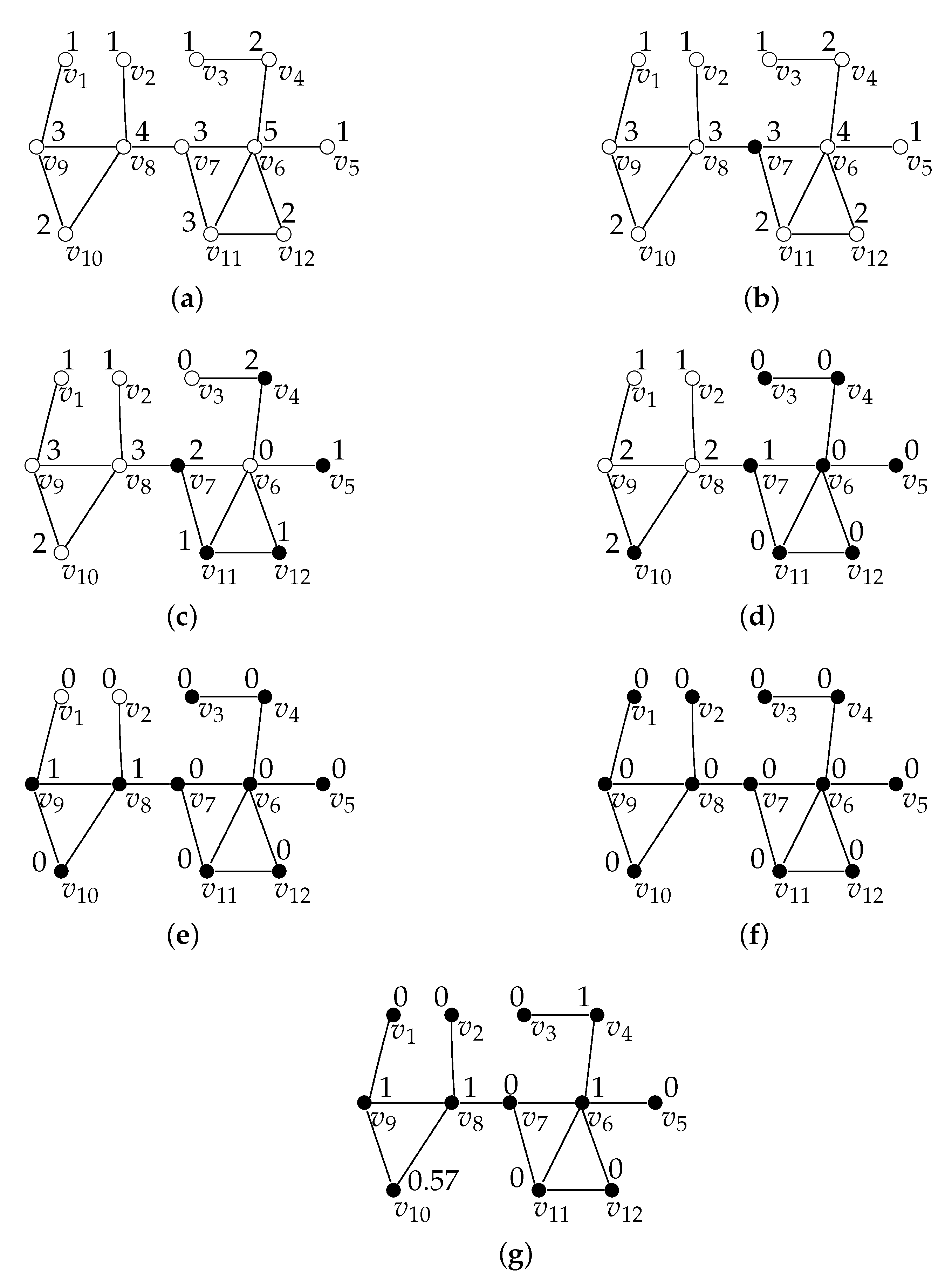
First, we illustrate the execution of Algorithm 1 with an example in Figure 1, where and . Figure 1a is the topology graph of the network with , the of each vertex is marked on the graph, initial values of variables , , are shown in Table 1. In Figure 1b, when and , satisfy , are active vertices, hence are selected, then the corresponding of are changed from 0 to . According to lines 20–22 of Algorithm 1, satisfies , hence is colored black and we need to update . New values of variables , , , , are shown in Table 1. When , new values of variables , , , are shown in Table 1, we continue to execute the algorithm, and are colored black in Figure 1c. When , the dynamic degrees of all vertices are less than the corrsponding , so the outer iteration ends, and we update in Table 1. By continuing to execute Algorithm 1, when and , the coloring process of all vertices and the changes in are shown in Figure 1d–f. Initially, all . By executing the algorithm, the final of all vertices is shown in Figure 1g. So, we can determine that the size of the output solution of Algorithm 1 is .
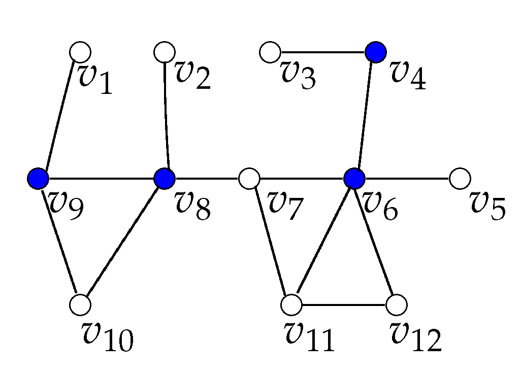
The optimal TDS for this example is shown in Figure 2. Hence, we can see that the optimal TDS in this case is , so its size is 4. The performance ratio of Algorithm 1 is in this case.
Second, we give some lemmas that will be used to analyze the approximation ratio of Algorithm 1.
| Algorithm 1 Approximating |
Input: Given a graph , a positive integer k. Output: A feasible solution for .
|
Lemma 1.
When each outer loop iteration ℏ starts, for each vertex , we can obtain
Proof of Lemma 1.
We prove it by using induction.
Firstly, when , the condition . Due to being the dynamic degree in and being the maximum degree, it is clear that .
Secondly, in order to prove that the other iterations also hold, we use the algorithm in [37] to approximate (the modified algorithm will be available in Appendix A), where all vertices know in their algorithm. Thus, similar to their algorithmic analysis, in the last step () of the preceding outer loop iteration , the of all vertices with is changed to 1. Hence, all vertices in will be colored black, so will be changed to 0. Thus, the dynamic degrees of all vertices with is changed to 0, and the dynamic degrees of the other vertices clearly satisfy this inequality . Therefore, by using the algorithm in [37], we can verify that holds when each outer loop iteration ℏ starts. Hence, for our algorithm, we only need to show that the of all vertices with is changed to 1 when each inner loop iteration ends (). According to lines 17–19 of Algorithm 1, we can see that the of all vertices with are changed to 1 when . Therefore, we only need to prove that for each vertex .
Based on the induction hypothesis, we can obtain, for each vertex , in each outer loop iteration start. As is the maximum dynamic degree in the second neighborhood of , we can obtain for each vertex . Hence, we have
We complete the proof. □
Lemma 2.
Before assigning a new to , for each vertex , we can obtain
Proof of Lemma 2.
We also prove it by using induction.
Firstly, when , . According to the definitions of and , it is clear that .
Secondly, when , we need to prove that all vertices with are colored black when the inner loop iteration ends. We apply the induction hypothesis to the other inner loop iterations, so we can obtain for each vertex . Hence, the of each active vertex is assigned in line 17 as
If each vertex has more than active vertices in , will be covered. So, the conclusion holds. □
Then, we analyze all the increased in the inner loop iterations. It is difficult to directly compute the sum of all the increased . Therefore, for each vertex , we introduce a new variable . All is initialized as 0 in line 4 of Algorithm 1. When the vertex increases the over time, the increased is equally distributed to the of the vertices in {∣ which is colored white before the increment of at line 17}. Hence, we can obtain that is equal to the sum of all the increased in each outer loop iteration. So, we only need to show that all are bounded, as then all the increased are also bounded.
Lemma 3.
For each vertex , we can obtain when each outer loop iteration ends.
Proof of Lemma 3.
Due to all in line 4, we only need to analyze a single outer loop iteration ℏ. From the execution of the algorithm, we know that all are increased in line 17. Therefore, can only be increased there if the vertex is white. For each white vertex , we need to discuss two cases during the current outer loop ℏ. The first case is that, when all inner loop iterations end, is still white. The second case is that, when the remaining inner loop iterations end, the vertex is or becomes black.
For the first case, we can easily obtain . Since all the increased x are distributed among at least , we can obtain
where the second inequality holds because and denote the maximum dynamic degree in and the second neighborhood of , respectively, so we have .
In the second case, we can see that only white vertices can increase their z. Since the will become smaller over time, these active vertices become active in the previous iterations. Hence, we can see that each active vertex contributes to the at most
Due to having active vertices in , the upper bound of the increased is
where the first inequality follows from .
Based on the two lemmas, we will analyze the correctness, approximation ratio, and time complexity of Algorithm 1 in the following. Firstly, we show that the algorithm outputs a feasible solution to the linear programming relaxation of the minimum total dominating set problem.
Theorem 1.
The output result of Algorithm 1 is a feasible solution to linear programming relaxation of minimum total dominating set problem .
Proof of Theorem 1.
According to the execution of Algorithm 1, will be colored ’black’ only when the vertex satifies , i.e., belongs to the feasible solution of . For each vertex , we can obtain and at the end of the iteration (), so the algorithm will terminate and all vertices are colored ’black’. Hence, the output result of Algorithm 1 is a feasible solution for . □
Secondly, we analyze the approximation ratio of Algorithm 1.
Theorem 2.
For a given network graph G and a positive integer k, Algorithm 1 is a -approximation for the minimum total dominating set problem in G.
Proof of Theorem 2.
According to the above description of , is equal to the sum of all the increased in each outer loop iteration of Algorithm 1. From Lemma 3, we know that the of all vertices satisfy when each outer loop iteration ends. So, for each vertex , the sum of the in of the vertex in the outer loop iteration is at most
where the second inequality holds because is the maximum dynamic degree in , , hence . The fourth inequality follows from Lemma 1, .
Next, for each vertex , if we let , then we can see that holds for each vertex ; hence, the is a feasible solution of . According to the weak duality theorem of linear programming, we can see that is a lower bound of an optimal TDS (). Therefore, for each outer loop iteration, we can obtain
On the other hand, there are k iterations in the outer loop. So, we can obtain
We complete the proof. □
Finally, we analyze the running time of Algorithm 1.
Theorem 3.
The number of communication rounds for Algorithm 1 is .
Proof of Theorem 3.
Firstly, it can be seen from the execution of the algorithm that every inner loop iteration needs to send four messages to all its neighbors in the algorithm, and there are k inner loop iterations, so it takes communication rounds. Secondly, every outer loop iteration needs to send two messages to all neighbors in the algorithm; hence, it takes communication rounds for each outer loop iteration. There are k outer loop iterations, so it takes communication rounds for all outer loop iterations. Finally, we need to calculate some values before the outer loop iteration starts, which takes communication rounds. Hence, we can see that the number of communication rounds in the algorithm is . □
5. Conclusions
In this paper, we present a distributed approximation algorithm for the total dominating set problem by using the maximum dynamic degree in the second neighborhood of the vertex and LP relaxation techniques. Our algorithm obtained only a relaxed solution; further considerations can be given on how to design a random rounding algorithm to obtain an integer TDS from the relaxed solution. It is interesting to consider this problem in wireless networks so that we can take advantage of the specificity of wireless networks to improve the performance of the algorithm. In practical applications, if the vertices in a graph are weighted, additional considerations could include how to design an approximation algorithm to solve the minimum total dominating set problem.
Author Contributions
Conceptualization, L.W.; methodology, L.W.; validation, L.W. and W.W.; formal analysis, L.W. and W.W.; investigation, L.W. and W.W.; writing—review and editing, L.W.; project administration, L.W. All authors have read and agreed to the published version of the manuscript.
Funding
The first author is supported by NSFC (No. 62272215).
Institutional Review Board Statement
Not applicable.
Data Availability Statement
This manuscript has no associated data.
Conflicts of Interest
The authors declare no conflict of interest.
Abbreviations
The following abbreviations are used in this manuscript:
| LP | Linear programming |
| TDS | Total dominating set |
| MTDS | Minimum total dominating set |
| Integer linear programming of minimum total dominating set problem | |
| Linear programming relaxation of minimum total dominating set problem | |
| Dual linear programming of minimum total dominating set problem | |
| Optimal total dominating set |
Appendix A
| Algorithm A1 Approximating |
Input: , a positive integer k and maximum degree . Output: A feasible solution for .
|
References
- Jiang, P.; Liu, J.; Wu, F.; Wang, J.; Xue, A. Node deployment algorithm for underwater sensor networks based on connected dominating set. Sensors 2016, 16, 388. [Google Scholar] [CrossRef] [PubMed] [Green Version]
- Chen, J.; He, K.; Du, R.; Zheng, M.; Xiang, Y.; Yuan, Q. Dominating set and network coding-based routing in wireless mesh networks. IEEE Trans. Parallel Distrib. Syst. 2013, 26, 423–433. [Google Scholar] [CrossRef]
- Fellows, M.R.; Koblitz, N. Combinatorially based cryptography for children (and adults). Congr. Numer. 1994, 99, 9–41. [Google Scholar]
- Kwon, S.; Kang, J.S.; Yeom, Y. Analysis of public-key cryptography using a 3-regular graph with a perfect dominating set. In Proceedings of the IEEE Region 10 Symposium (TENSYMP), Grand Hyatt Jeju, Republic of Korea, 23–25 August 2021; pp. 1–6. [Google Scholar]
- Allesina, S.; Bodini, A. Who dominates whom in the ecosystem? Energy flow bottlenecks and cascading extinctions. J. Theor. Biol. 2004, 230, 351–358. [Google Scholar] [CrossRef]
- Haynes, T.W.; Hedetniemi, S.M.; Hedetniemi, S.T.; Henning, M.A. Domination in graphs applied to electric power networks. SIAM J. Discret. Math. 2002, 15, 519–529. [Google Scholar] [CrossRef]
- Haynes, T.W.; Hedetniemi, S.; Slater, P. Fundamentals of Domination in Graphs; CRC Press: Boca Raton, FL, USA, 2013. [Google Scholar]
- Haynes, T.W. Domination in Graphs: Volume 2: Advanced Topics; Routledge: London, UK, 2017. [Google Scholar]
- Haynes, T.W.; Hedetniemi, S.; Henning, M.A. Topics in Domination in Graphs; Springer Nature: Berlin/Heidelberg, Germany, 2020. [Google Scholar]
- Haynes, T.W.; Hedetniemi, S.; Henning, M.A. Structures of Domination in Graphs; Springer: Cham, Switzerland, 2021. [Google Scholar]
- Alzoubi, K.M.; Wan, P.J.; Frieder, O. Maximal independent set, weakly-connected dominating set, and induced spanners in wireless ad hoc networks. Int. J. Found. Comput. Sci. 2003, 14, 287–303. [Google Scholar] [CrossRef]
- Das, B.; Bharghavan, V. Routing in ad-hoc networks using minimum connected dominating sets. In Proceedings of the ICC’97-International Conference on Communications, Montreal, QC, Canada, 8–12 June 1997; pp. 376–380. [Google Scholar]
- Belhoul, Y.; Yahiaoui, S.; Kheddouci, H. Efficient self-stabilizing algorithms for minimal total k-dominating sets in graphs. Inf. Process. Lett. 2014, 114, 339–343. [Google Scholar] [CrossRef]
- Cockayne, E.J.; Dawes, R.M.; Hedetniemi, S.T. Total domination in graphs. Networks 1980, 10, 211–219. [Google Scholar] [CrossRef]
- Awerbuch, B.; Goldberg, A.V.; Luby, M.; Plotkin, S.A. Network decomposition and locality in distributed computation. In Proceedings of the 30th Annual IEEE Symposium on Foundations of Computer Science, Research Triangle Park, NC, USA, 30 October–1 November 1989; pp. 364–369. [Google Scholar]
- Alipour, S.; Futuhi, E.; Karimi, S. On distributed algorithms for minimum dominating set problem, from theory to application. arXiv 2020, arXiv:2012.04883. [Google Scholar] [CrossRef]
- Alipour, S.; Jafari, A. A local constant approximation factor algorithm for minimum dominating set of certain planar graphs. In Proceedings of the 32nd ACM Symposium on Parallelism in Algorithms and Architectures, Virtual, 15–17 July 2020; pp. 501–502. [Google Scholar]
- Haynes, T.W.; Hedetniemi, S.T.; Slater, P.J. Fundamentals of Domination in Graphs; Chapman and Hall/CRC: New York, NY, USA, 1998. [Google Scholar]
- Haynes, T.W.; Hedetniemi, S.T.; Slater, P.J. Domination in Graphs: Advanced Topics; Chapman and Hall/CRC Pure and Applied Mathematics Series; Marcel Dekker: New York, NY, USA, 1998; Volume 209. [Google Scholar]
- Henning, M.A. A survey of selected recent results on total domination in graphs. Discret. Math. 2009, 309, 32–63. [Google Scholar] [CrossRef] [Green Version]
- Henning, M.A.; Yeo, A. Total Domination in Graphs; Springer: New York, NY, USA, 2013. [Google Scholar]
- Garey, M.R.; Johnson, D.S. Computers and Intractability: A Guide to the Theory of NP-Completeness; Freeman: San Francisco, CA, USA, 1978. [Google Scholar]
- Khanna, S.; Motwani, R.; Sudan, M.; Vazirani, U. On syntactic versus computational views of approximability. SIAM J. Comput. 1998, 28, 164–191. [Google Scholar] [CrossRef] [Green Version]
- Papademitriou, C.; Yannakakis, M. Optimization, approximation and complexity classes. In Proceeding of the 20th Annual ACM Symposium on Theory of Computing, Chicago, IL, USA, 2–4 May 1988; pp. 229–234. [Google Scholar]
- Crescenzi, P.; Kann, V. A Compendium of NP Optimization Problems; Technical Report SI/RR-95/02; Department of Computer Science, University of Rome “La Sapienza”: Rome, Italy, 1995. [Google Scholar]
- Laskar, R.; Pfaff, J.; Hedetniemi, S.M.; Hedetniemi, S.T. On the algorithmic complexity of total domination. SIAM J. Algebr. Discret. Methods 1984, 5, 420–425. [Google Scholar] [CrossRef]
- Henning, M.A.; Yeo, A. A transition from total domination in graphs to transversals in hypergraphs. Quaest. Math. 2007, 30, 417–436. [Google Scholar] [CrossRef]
- Chlebík, M.; Chlebíková, J. Approximation hardness of dominating set problems in bounded degree graphs. Inf. Comput. 2008, 206, 1264–1275. [Google Scholar] [CrossRef] [Green Version]
- Zhu, J. Approximation for minimum total dominating set. In Proceedings of the 2nd International Conference on Interaction Sciences: Information Technology, Culture and Human, Seoul, Republic of Korea, 24–26 November 2009; Association for Computing Machinery: New York, NY, USA, 2009; pp. 119–124. [Google Scholar]
- Schaudt, O.; Schrader, R. The complexity of connected dominating sets and total dominating sets with specified induced subgraphs. Inf. Process. Lett. 2012, 112, 953–957. [Google Scholar] [CrossRef]
- Yuan, F.; Li, C.; Gao, X.; Yin, M.; Wang, Y. A novel hybrid algorithm for minimum total dominating set problem. Mathematics 2019, 7, 222. [Google Scholar] [CrossRef] [Green Version]
- Bahadir, S. An algorithm to check the equality of total domination number and double of domination number in graphs. Turk. J. Math. 2020, 44, 1701–1707. [Google Scholar] [CrossRef]
- Hu, S.; Liu, H.; Wang, Y.; Li, R.; Yin, M.; Yang, N. Towards efficient local search for the minimum total dominating set problem. Appl. Intell. 2021, 51, 8753–8767. [Google Scholar] [CrossRef]
- Jena, S.K.; Das, G.K. Total domination in geometric unit disk graphs. In Proceeding of the 33rd Canadian Conference on Computational Geometry (CCCG), Halifax, NS, Canada, 10–12 August 2021; pp. 219–227. [Google Scholar]
- Hochbaum, D.S.; Maass, W. Approximation schemes for covering and packing problems in image processing and VLSI. J. ACM (JACM) 1985, 32, 130–136. [Google Scholar] [CrossRef] [Green Version]
- Goddard, W.; Hedetniemi, S.T.; Jacobs, D.P.; Srimani, P.K. A self-stabilizing distributed algorithm for minimal total domination in an arbitrary system graph. In Proceedings of the International Parallel and Distributed Processing Symposium, Nice, France, 22–26 April 2003. [Google Scholar]
- Elkin, M. Distributed approximation: A survey. ACM SIGACT News 2004, 35, 40–57. [Google Scholar] [CrossRef]
- Kuhn, F.; Wattenhofer, R. Constant-time distributed dominating set approximation. Distrib. Comput. 2005, 17, 303–310. [Google Scholar] [CrossRef] [Green Version]
- Jia, L.; Rajaraman, R.; Suel, T. An efficient distributed algorithm for constructing small dominating sets. Distrib. Comput. 2002, 15, 193–205. [Google Scholar] [CrossRef]
- Guha, S.; Khuller, S. Approximation algorithms for connected dominating sets. Algorithmica 1998, 20, 374–387. [Google Scholar] [CrossRef] [Green Version]
Figure 1.
An illustration of Algorithm 1, in which and . (a) is the topology graph, of each vertex is marked on the graph. (b) When and , is colored black and we update . (c) When and , are colored black and we update . (d) When and , are colored black and we update . (e) When and , are colored black and we update . (f) When and , are colored black and we update . By executing the algorithm, the final of all vertices is shown in (g).

Figure 2.
The optimal total dominating set, in which and .


Table 1.
Initial and new values of some variables.
| 0 | 0 | 0 | 0 | 0 | 0 | 0 | 0 | 0 | 0 | 0 | 0 | ||
| initial | 1 | 1 | 1 | 2 | 1 | 5 | 3 | 4 | 3 | 2 | 3 | 2 | |
| 4 | 4 | 5 | 5 | 5 | 4 | 5 | 5 | 4 | 4 | 5 | 5 | ||
| 3.03 | 3.03 | 3.62 | 3.62 | 3.62 | 3.03 | 3.62 | 3.62 | 3.03 | 3.03 | 3.62 | 3.62 | ||
| 0 | 1 | 0 | 1 | 1 | 0 | 2 | 0 | 1 | 1 | 1 | 1 | ||
| 1 | 0 | 1 | 0 | 0 | 2 | 1 | 2 | 1 | 1 | 2 | 1 | ||
| 0 | 0 | 0 | 0 | 0 | 0.57 | 0 | 0.57 | 0 | 0 | 0 | 0 | ||
| 1 | 1 | 1 | 2 | 1 | 4 | 3 | 3 | 3 | 2 | 2 | 2 | ||
| 0 | 0 | 0 | 1 | 1 | 0 | 0 | 0 | 0 | 0 | 1 | 1 | ||
| 0 | 0 | 1 | 0 | 0 | 1 | 1 | 0 | 0 | 0 | 1 | 1 | ||
| 0 | 0 | 0 | 0 | 0 | 1 | 0 | 0.57 | 0 | 0 | 0 | 0 | ||
| 1 | 1 | 0 | 2 | 1 | 0 | 2 | 3 | 3 | 2 | 1 | 1 | ||
| 3 | 3 | 2 | 2 | 2 | 3 | 3 | 3 | 3 | 3 | 3 | 2 |
Disclaimer/Publisher’s Note: The statements, opinions and data contained in all publications are solely those of the individual author(s) and contributor(s) and not of MDPI and/or the editor(s). MDPI and/or the editor(s) disclaim responsibility for any injury to people or property resulting from any ideas, methods, instructions or products referred to in the content. |
© 2023 by the authors. Licensee MDPI, Basel, Switzerland. This article is an open access article distributed under the terms and conditions of the Creative Commons Attribution (CC BY) license (https://creativecommons.org/licenses/by/4.0/).
Share and Cite
MDPI and ACS Style
Wang, L.; Wang, W. An Approximation Algorithm for a Variant of Dominating Set Problem. Axioms 2023, 12, 506. https://doi.org/10.3390/axioms12060506
AMA Style
Wang L, Wang W. An Approximation Algorithm for a Variant of Dominating Set Problem. Axioms. 2023; 12(6):506. https://doi.org/10.3390/axioms12060506
Chicago/Turabian StyleWang, Limin, and Wenqi Wang. 2023. "An Approximation Algorithm for a Variant of Dominating Set Problem" Axioms 12, no. 6: 506. https://doi.org/10.3390/axioms12060506
Note that from the first issue of 2016, this journal uses article numbers instead of page numbers. See further details here.