Article

An Analytic Solution for the Dynamic Behavior of a Cantilever Beam with a Time-Dependent Spring-like Actuator

1
Department of Aircraft Engineering, Air Force Institute of Technology, 1 Julun Road, Gang-Shan District, Kaohsiung City 820, Taiwan
2
Department of Mechanical Engineering, Air Force Institute of Technology, 1 Julun Road, Gang-Shan District, Kaohsiung City 820, Taiwan
3
Department of Aircraft Maintenance, Far East University, 49 Zhonghua Road, Xinshi District, Tainan City 744, Taiwan
*
Author to whom correspondence should be addressed.
Axioms 2023, 12(5), 500; https://doi.org/10.3390/axioms12050500
Submission received: 17 February 2023 / Revised: 6 May 2023 / Accepted: 16 May 2023 / Published: 19 May 2023
(This article belongs to the Special Issue Computational and Mathematical Methods in Science and Engineering)

Abstract

:
The purpose of this study is to derive an analytical solution for a cantilever beam with a novel spring-like actuator that behaves like a time-dependent spring and to study the dynamic behavior of the system. A time-dependent spring was set at the free end of the cantilever beam to model the novel spring-like actuator. First, the boundary conditions were transformed from being nonhomogeneous to being homogeneous using the shifting function method. The solution of the analytic series was then obtained by using the expansion theorem method. The correctness of the proposed analytical solution was verified by comparing the results with those obtained via the separation of variables in the special extreme case of a constant spring coefficient. We took the free end of a cantilever beam with harmonic spring stiffness and an external periodic unit load as an example. The influence of the actuator parameters, such as the effect of the magnitude and the frequency of the time-dependent spring stiffness on the resonance frequency, was investigated. An important new result was found, i.e., that the resonance frequency is clearly dependent on the magnitude and the frequency of the spring-like actuator in the first two modes, but not in the third and fourth modes. In practical engineering applications, system resonance can be avoided by adjusting the magnitude and frequency of the actuator.
MSC:
35A25; 37N15; 70G60; 74H10; 74H45; 74K10

1. Introduction

With the rapid development of mechatronics, typical examples such as micro-actuators, micro-generators, micro-switches, and micro-beams have been used to manufacture the various structures and models of cantilever beams [1,2,3,4,5,6]. Meanwhile, smart materials have been developed in recent decades and these can be used to manufacture controller components [7,8,9,10,11,12,13]. With the development trend of mechatronics and smart materials, it is assumed that in the future researchers will be able to design and fabricate a new type of spring-like actuator (Figure 1), which can work like a time-dependent spring with a fast dynamic response (Figure 2). Therefore, a novel cantilever beam with a free end supported by a time-dependent spring is proposed. Several books [14,15] have presented and derived the governing equations of motion for beams with different boundary conditions; however, no analytical solutions have been presented for a cantilever beam with a time-dependent spring-like actuator. In this study, an analytical solution of the undamped forced vibration of a beam system with a time-dependent spring was achieved and its dynamic behavior and parameters were investigated in detail.
Although none of the previous literature has focused on this topic, the classical problem of a beam’s vibration with time-dependent boundary conditions (usually occurring in the spring design, the dynamic analysis of tires, and the suppression of shock in landing gear) has been studied by many researchers since the 1940s, including Nothmann in 1948 [16] and Lee and Yan in 2015 [17]. The time-dependent boundary conditions of such beams mainly include both geometric (deflection or slope) and natural (shear force or moment) conditions. The solutions to the problems can be generated using either the Laplace transform method (see, e.g., Nothmann [16] and Yen and Kao [18]) or the expansion theorem method (see, e.g., Mindlin and Goodman [19] and Lee and Yan [17]). Nothmann and Yen and Kao used the Laplace transform method to solve the vibration of a cantilever beam with prescribed end motion and the vibration of beam–mass systems with time-dependent boundary conditions, respectively. The main difficulty in using the Laplace transform method, however, lies in the inversion process, which involves the evaluation of an integral in most transforms. Therefore, few studies ([16,18]) have used the Laplace transform method, while the expansion theorem method has been more frequently applied in other studies.
For example, Mindlin and Goodman used the expansion theorem method, along with four fifth-order shifting polynomial functions (the M–G method), to change the variables and to transform a mathematical problem with nonhomogeneous boundary conditions into one with homogeneous boundary conditions. The idea that one could choose dependent variables with the result that boundary conditions and partial differential equations could still hold homogeneous boundaries was suggested by Edstorm [20]. By extending that idea and resolving Nothmann’s example, Grant [21] stated that the solution could easily be obtained without the difficulty of finding the Laplace inverse transforms. Later, the M–G method was used by Herrmann [22] to analyze the behavior of the forced vibration of Timoshenko beams, by Berry and Nagdhi [23] to investigate elastic bodies with time-dependent boundary conditions, and by Epstein [24] to study the Bernoulli–Euler beams with internal time-dependent boundaries. In addition, Aravamudan and Murthy [25] combined the perturbation method, the Galerkin method, and the M–G method to study the nonlinear vibration of beams with time-dependent boundary conditions. In the 1990s, Lee and Lin [26,27,28] and Lin [29] proposed the shifting function method, which modified the M–G method to analyze Bernoulli–Euler beams, Timoshenko beams, and pre-twisted nonuniform beams with time-dependent boundary conditions. Lee et al. [30] extended the prior studies and considered the transverse vibration problem to develop a set of shifting functions that consisted of fundamental solutions of nonuniform beams and to discuss the physical meaning of the shifting functions. Recently, the shifting function method was extended by Lee and Yan [17] to derive the exact deflection of an out-of-plane curved Timoshenko beam with nonlinear boundary conditions.
Sajjadi et al. [31] developed a nonlinear meniscus force and applied it to a trolling-mode atomic force microscope nanoneedle. A multiple time scales method was employed to derive the analytical solution to the distributed parameter system. The analytical solution was compared with the experimental data and the finite element solution in order to assess the accuracy of the method. Horssen et al. [32] showed why the variable separation method cannot solve the wave problems on a fixed bounded interval that involves a Dirichlet-type boundary condition at one end and a Robin-type boundary condition with a time-varying spring coefficient at the other end. The d’Alembert formula was used to solve this problem. Ahmad et al. [33] investigated the vibrational behavior of rectangular and V-shaped atomic force microscopy microcantilevers with an extended piezoelectric layer using the finite element method. A nonlinear spring was used in finite element modeling to simulate the nonlinear attraction–repulsion interaction between the tip and the sample. The simulation results of the three-dimensional finite element method were verified by comparison with the experimental and analytical results. An initial boundary value problem for a forced string equation was studied by Wang et al. [34]. The string was also on a fixed bounded interval, and the boundary conditions consisted of a slowly varying time-dependent spring coefficient of Robin type at one end and of Dirichlet type at the other end. An adapted version of the variable separation method, the averaging, and perturbation techniques were applied in order to solve resonance problems. Wang et al. [35] studied a robot structure with a time-dependent stiffness. The vibration-driven robot was excited with sinusoidal stiffness. The incremental harmonic balance method was employed to evaluate the response.
The purpose of this paper is to analytically solve the dynamic behavior of a cantilever beam with a time-dependent spring support at the free end using the shifting function method combined with the expansion theorem method. To the best of the authors’ knowledge, no literature has investigated the beam vibration with a time-dependent spring support. In this paper, the dynamic response of the novel spring-like actuator was analyzed using the generated closed solution of a Bernoulli–Euler beam with a time-dependent spring support at the free end. The governing equation of this problem was a fourth-order ordinary differential equation with nonhomogeneous boundary conditions. The boundary conditions were transformed from nonhomogeneous into homogeneous by using the shifting function method that did not require any integral transformation. The shifting function derived in this study was a quartic polynomial function. Then, we applied the expansion theorem to solve the differential equation, and the analytical solution was obtained in the form of a series. The correctness of the proposed analytical solution was verified by comparing it with the results obtained by the separation of variables method in the special extreme case of a constant spring coefficient. The dynamic behavior of the system was analyzed in detail by considering the harmonic function of time as a time-dependent spring coefficient.
The novelty and contributions of this paper are as follows:
(1)
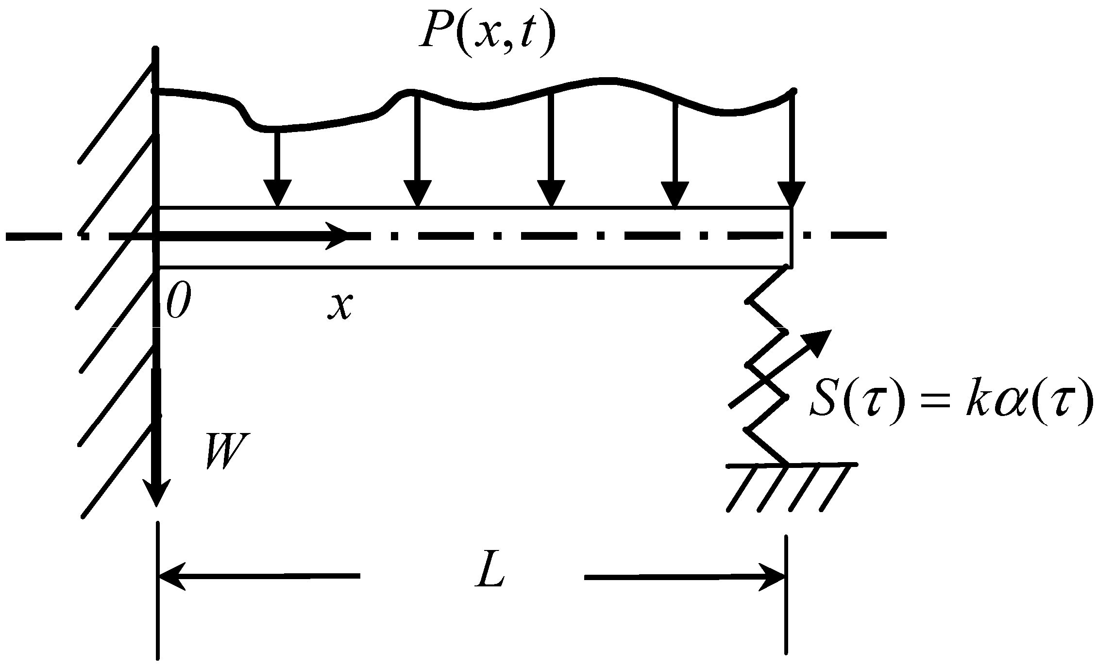
The novelty of this study comes from the fact this is the first investigation of the dynamic behavior of a cantilever beam with a time-dependent spring support at the free end.
(2)
The proposed method, combining the shifting function method with the expansion theorem method, can efficiently find the analytic solution to the dynamic problem of a time-dependent spring-supported cantilever beam.
(3)
The influence of time-dependent spring coefficients on the beam system has been obtained and discussed.

2. Mathematical Modeling

To evaluate the dynamic behavior of the novel spring-like actuator, the actuator is set up at the free end of a Bernoulli–Euler cantilever beam with a uniform cross section (Figure 1). The actuator is modeled as a spring support with a time-dependent medium, and the beam is assumed to be loaded laterally (Figure 2). The governing equation, boundary and initial conditions can be expressed as follows [14,15]:
E I 4 W ( x , t ) x 4 + ρ A 2 W ( x , t ) t 2 = P ( x , t ) , 0 < x < L , t > 0 ,
W ( 0 , t ) = 0 ,   W ( 0 , t ) x = 0 ,   at   x = 0 ,
2 W ( L , t ) x 2 = 0 ,   E I 3 W ( L , t ) x 3 K ( t ) W ( L , t ) = 0 ,   at   x = L ,
W ( x , 0 ) = W 0 ( x ) ,   W ( x , 0 ) t = W ¯ 0 ( x ) ,   when   t = 0 ,
where W ( x , t ) is the flexural displacement, x is the coordinate along the centerline of the beam, t is the time, and L is the beam length. E , I , and A denote the Young’s modulus, the area moment of inertia, and the cross-sectional area, respectively. ρ is the mass density and P ( x , t ) is the applied transverse force per unit length. K ( t ) denotes a time-dependent spring function; W 0 ( x ) and W ¯ 0 ( x ) are the initial deflection and initial velocity, respectively.
Using the dimensionless approach, we define the following quantities
ξ = x L ,   w ( ξ ,   τ ) = W ( x ,   t ) L ,   τ = t L 2 E I ρ A ,   p ( ξ ,   τ ) = P ( x ,   t ) L 3 E I ,
w 0 ( ξ ) = W 0 ( x ) L ,   w ¯ 0 ( ξ ) = W ¯ 0 ( x ) L ,   S ( τ ) = K ( t ) L 3 E I .
The governing differential equation and the associated boundary conditions for the system can be derived as
w ( ξ ,   τ ) + w ¨ ( ξ ,   τ ) = p ( ξ ,   τ ) ,
w ( 0 ,   τ ) = 0 ,   w ( 0 ,   τ ) = 0 ,
w ( 1 ,   τ ) = 0 ,   w ( 1 ,   τ ) = S ( τ ) w ( 1 ,   τ ) = k α ( τ ) w ( 1 , τ ) ,
where α ( τ ) and k represent the unit time function and the magnitude of the dimensionless time-dependent spring stiffness. It is noted that the primes and the dots are used to denote differentiation with respect to the dimensionless position ξ and the dimensionless time τ , respectively. The dimensionless initial conditions are specified as two arbitrary functions
w ( ξ ,   0 ) = w 0 ( ξ ) ,   w ˙ ( ξ ,   0 ) = w ¯ 0 ( ξ ) .

3. The Solution Methodology

3.1. The Shifting Function Method

To find the solution of the beam vibration system, the shifting function method [26,27,28] is adopted by taking
w ( ξ ,   τ ) = v ( ξ ,   τ ) + g ( ξ ) f ( τ ) ,
where v ( ξ ,   τ ) is the transformed function, g ( ξ )   is the shifting function to be specified, and f ( τ ) is defined as
f ( τ ) = S ( τ ) w ( 1 ,   τ ) .
Substituting Equation (10) into Equations (6)–(9), the partial differential equation is derived as
v ( ξ ,   τ ) + v ¨ ( ξ ,   τ ) = p ( ξ ,   τ ) g ( ξ ) f ( τ ) g ( ξ ) f ¨ ( τ ) ,
and the boundary conditions are
v ( 0 ,   τ ) = g ( 0 ) f ( τ ) ,   v ( 0 ,   τ ) = g ( 0 ) f ( τ ) ,
v ( 1 ,   τ ) = g ( 1 ) f ( τ ) ,   v ( 1 ,   τ ) = [ 1 g ( 1 ) ] f ( τ ) .
Additionally, the corresponding initial conditions now become
v ( ξ ,   0 ) = w 0 ( ξ ) g ( ξ ) f ( 0 ) ,
v ˙ ( ξ ,   0 ) = w ¯ 0 ( ξ ) g ( ξ ) f ˙ ( 0 ) .
Since there are two variables v ( ξ ,   τ ) and f ( τ ) in Equation (12), the boundary value problem cannot be solved directly via an analytical method. The relationship between them is deduced below.
The shifting function g ( ξ ) is chosen to satisfy the following ordinary differential equation with five boundary conditions by changing Equations (13) and (14) from nonhomogeneous into homogeneous boundary conditions.
g ( ξ ) = C ,
g ( 0 ) = 0 ,   g ( 0 ) = 0 ,   g ( 1 ) = 0 ,   g ( 1 ) = 1 ,   g ( 1 ) = 0 ,
where C is a constant to be determined. The fifth condition in Equation (18) is added to construct a relationship between w ( 1 ,   τ ) and v ( 1 ,   τ ) .
By solving Equations (17) and (18), the translation function and constant C can be obtained as
g ( ξ ) = 2 ξ 4 5 ξ 3 + 3 ξ 2 18 ,
C = 8 3 .
Substituting the shifting function back into Equation (10) yields
w ( ξ ,   τ ) = v ( ξ ,   τ ) + 2 ξ 4 5 ξ 3 + 3 ξ 2 18 f ( τ ) .
Then, setting ξ = 1 in the above equation gives the relationship
w ( 1 ,   τ ) = v ( 1 ,   τ ) .
As a result, using this relationship, the two variables in Equation (12) are integrated into one. Therefore, according to Equations (11) and (22), Equation (12) can be rewritten in terms of the transformed function as follows:
v ( ξ ,   τ ) + v ¨ ( ξ ,   τ ) = p ( ξ , τ ) 8 3 k α ( τ ) v ( 1 ,   τ ) k g ( ξ ) [ α ( τ ) v ¨ ( 1 , τ ) + 2 α ˙ ( τ ) v ˙ ( 1 , τ ) + α ¨ ( τ ) v ( 1 , τ ) ] .
The right-hand side of the above equation represents the forced terms of the transformed system; the associated boundary conditions, Equations (13) and (14), thus become homogeneous as
v ( 0 ,   τ ) = 0 ,   v ( 0 ,   τ ) = 0 ,
v ( 1 ,   τ ) = 0 ,   v ( 1 ,   τ ) = 0 .
Under these boundary conditions, v ( ξ ,   τ ) exactly represents the deflection of the cantilever beam. Rearranging Equations (15) and (16), the corresponding initial conditions become
v ( ξ ,   0 ) = w 0 ( ξ ) k g ( ξ ) α ( 0 ) v ( 1 ,   0 ) ,
v ˙ ( ξ ,   0 ) = w ¯ 0 ( ξ ) k g ( ξ ) [ α ( 0 ) v ˙ ( 1 ,   0 ) + α ˙ ( 0 ) v ( 1 , 0 ) ] .

3.2. The Expansion Theorem Method

The method of eigenfunction expansion is used to solve the boundary value problem of v ( ξ ,   τ ) (Equations (23)–(25)), and the corresponding eigenfunctions are obtained through homogeneous governing differential equations and homogeneous boundary conditions.
In order to derive the orthogonality condition for the system eigenfunctions, the following trial function will be used
ϕ n ( ξ ) = ϕ n o r [ sin λ n ξ sinh λ n ξ H n ( cos λ n ξ cosh λ n ξ ) ] ,   n = 1 ,   2 ,   3 ,
where H n is defined as
H n = sin λ n + sinh λ n cos λ n + cosh λ n
and the eigenvalues λ n s are the roots of the following transcendental equation
cos   λ n cosh   λ n + 1 = 0 .
In this case, the trial function is chosen such that the inner product is
0 1 ϕ m ( ξ ) ϕ n ( ξ ) d ξ = δ m n ,
where δ m n denotes the Kronecker delta and ϕ n o r in Equation (28) is defined as
ϕ n o r = ( cos λ n + cosh λ n ) [ ( cos 2 λ n + cosh 2 λ n + 4 sin λ n sinh λ n ) / 2 ] 1 2 .
By using the expansion theorem method, one can assume that the solution of Equation (23) is of the form
v ( ξ ,   τ ) = n = 1 ϕ n ( ξ ) q n ( τ )
where q n ( τ )     ( n = 1 ,   2 ,   3 , ) represents the time-dependent generalized coordinates. Substituting the solution of Equation (33) into Equation (23), one can obtain
n = 1 [ ϕ n     ( ξ ) q n ( τ ) + ϕ n ( ξ ) q ¨ n ( τ ) ] = p ( ξ , τ ) n = 1 { 8 3 k ϕ n ( 1 ) α ( τ ) q n ( τ ) + k ϕ n ( 1 ) g ( ξ ) [ α ( τ ) q ¨ n ( τ ) + 2 α ˙ ( τ ) q ˙ n ( τ ) + α ¨ ( τ ) q n ( τ ) ] } .
Expanding p ( ξ , τ ) on the right-hand side of Equation (34) in terms of series yields
n = 1 [ ϕ n     ( ξ ) q n ( τ ) + ϕ n ( ξ ) q ¨ n ( τ ) ] = n = 1 ϕ n ( ξ ) β n ( τ ) n = 1 { 8 3 k ϕ n ( 1 ) α ( τ ) q n ( τ ) + k ϕ n ( 1 ) g ( ξ ) [ α ( τ ) q ¨ n ( τ ) + 2 α ˙ ( τ ) q ˙ n ( τ ) + α ¨ ( τ ) q n ( τ ) ] }
where β n ( τ ) is defined as
β n ( τ ) = 0 1 ϕ n ( ξ ) p ( ξ ,   τ ) d ξ .
From Equation (35), one can obtain
ϕ n     ( ξ ) q n ( τ ) + ϕ n ( ξ ) q ¨ n ( τ ) = ϕ n ( ξ ) β n ( τ ) 8 3 k ϕ n ( 1 ) α ( τ ) q n ( τ ) k ϕ n ( 1 ) g ( ξ ) [ α ( τ ) q ¨ n ( τ ) + 2 α ˙ ( τ ) q ˙ n ( τ ) + α ¨ ( τ ) q n ( τ ) ] .
Now, by taking the inner product of any trial function ϕ n ( ξ ) in the above equation and integrating over the entire domain, the differential equation for q n ( τ ) can be obtained as follows:
q ¨ n ( τ ) + 2 δ n k α ˙ ( τ ) 1 + δ n k α ( τ ) q ˙ n ( τ ) + λ n 4 + γ n k α ( τ ) + δ n k α ¨ ( τ ) 1 + δ n k α ( τ ) q n ( τ ) = β n ( τ ) 1 + δ n k α ( τ )
where γ n and δ n are defined by the following expressions:
γ n = 8 3 ϕ n ( 1 ) 0 1 ϕ n ( ξ ) d ξ = 8 ϕ n ( 1 ) ϕ n o r 3 λ n [ H n ( sin λ n sinh λ n ) + cos λ n + cosh λ n 2 ] ,
δ n = ϕ n ( 1 ) 0 1 ϕ n ( ξ ) g ( ξ ) d ξ = ϕ n ( 1 ) ϕ n o r 3 λ n 5 { 8   [ 2 cos λ n cosh λ n H n ( sin λ n sinh λ n ) ] 3 λ n [ sin λ n sinh λ n H n ( cos λ n cosh λ n ) ] } .
It is worth noting that the coefficients of the q ˙ n ( τ ) term in Equation (38) exerts a damping effect.
Additionally, the initial functions w 0 ( ξ ) and w ¯ 0 ( ξ ) expand in series to
w 0 ( ξ ) = n = 1 η n ϕ n ( ξ ) ,   w ¯ 0 ( ξ ) = n = 1 ζ n ϕ n ( ξ ) ,
where η n and ζ n are defined as
η n = 0 1 ϕ n ( ξ ) w 0 ( ξ ) d ξ ,   ζ n = 0 1 ϕ n ( ξ ) w ¯ 0 ( ξ ) d ξ .
Now, the corresponding initial conditions in Equations (26) and (27) become
n = 1 ϕ n ( ξ ) q n ( 0 ) = n = 1 η n ϕ n ( ξ ) g ( ξ ) k α ( 0 ) n = 1 ϕ n ( 1 ) q n ( 0 ) ,
n = 1 ϕ n ( ξ ) q ˙ n ( 0 ) = n = 1 ζ n ϕ n ( ξ ) g ( ξ ) [ k α ( 0 ) n = 1 ϕ n ( 1 ) q ˙ n ( 0 ) + k α ˙ ( 0 ) n = 1 ϕ n ( 1 ) q n ( 0 ) ] .
In this case, let
ϕ n ( ξ ) q n ( 0 ) = η n ϕ n ( ξ ) ϕ n ( 1 ) g ( ξ ) k α ( 0 ) q n ( 0 ) ,
ϕ n ( ξ ) q ˙ n ( 0 ) = ζ n ϕ n ( ξ ) ϕ n ( 1 ) g ( ξ ) [ k α ( 0 ) q ˙ n ( 0 ) + k α ˙ ( 0 ) q n ( 0 ) ] .
After multiplying Equation (45) by ϕ n ( ξ ) and integrating over the domain, one can obtain
q n ( 0 ) = η n 1 + k α ( 0 ) δ n .
Likewise, performing the same operation and collecting the like terms in Equation (46) yields
q ˙ n ( 0 ) = ζ n 1 + k α ( 0 ) δ n η n δ n k α ˙ ( 0 ) [ 1 + k α ( 0 ) δ n ] 2 .
Finally, after solving Equation (38) with two initial conditions (Equations (47) and (48)), the complete solution for q n ( τ ) is obtained.

3.3. The Complete Solution and the Extreme Case Study

Substituting Equations (11), (22) and (33) back into Equation (10), the deflection of the cantilever beam with a time-dependent spring support is
w ( ξ ,   τ ) = n = 1 { [ ϕ n ( ξ ) + ϕ n ( 1 ) g ( ξ ) k α ( τ ) ] q n ( τ ) } .
Two extreme cases of the time-dependent spring coefficient are considered. One is a constant spring coefficient, and the other is zero spring stiffness. Their descriptions are as follows:
(A)
When considering a constant spring coefficient, i.e., S ( τ ) = k , Equation (38) becomes
q ¨ n ( τ ) + λ n 4 + k γ n 1 + k δ n q n ( τ ) = β n ( τ ) 1 + k δ n .
The corresponding two initial conditions in Equations (47) and (48) are
q n ( 0 ) = η n 1 + k δ n ,
q ˙ n ( 0 ) = ζ n 1 + k δ n .
Therefore, the solution in Equation (50) can be calculated as
q n ( τ ) = η n 1 + k δ n cos κ n τ + ζ n κ n ( 1 + k δ n ) sin κ n τ + 1 κ n ( 1 + k δ n ) 0 τ β n ( φ ) sin [ κ n ( τ φ ) ] d φ ,
where κ n is defined as
κ n = ( λ n 4 + k γ n 1 + k δ n ) 1 2 .
The dynamic deflection of a cantilever beam with a constant spring coefficient becomes
w ( ξ ,   τ ) = n = 1 { [ ϕ n ( ξ ) + k ϕ n ( 1 ) g ( ξ ) ] q n ( τ ) } .
(B)
If the spring stiffness k is equal to zero, i.e., the cantilever beam is only subjected to external loads, then Equation (53) becomes
q n ( τ ) = η n cos λ n 2 τ + ζ n λ n 2 sin λ n 2 τ + 1 λ n 2 0 τ β n ( φ ) sin [ λ n 2 ( τ φ ) ] d ϕ ,
and the dynamic deflection of the cantilever beam is now
w ( ξ ,   τ ) = n = 1 { ϕ n ( ξ ) q n ( τ ) } .
Then, the classical solution is derived.

4. Harmonic Excitation and Harmonic Type of a Time-Dependent Spring Support

The problem of cantilever beams with time-dependent supports and time-varying external loads is very important in practical engineering applications. Among various types of dynamic external loads, harmonic excitation is typical in mechanical design, and other general force situations can be solved by transforming them into harmonic forms through Fourier series expansion. Therefore, we assume that the external periodic unit load p ( ξ ,   τ ) at the free end of the cantilever beam is of the harmonic form
p ( ξ , τ ) =   δ ( ξ 1 ) cos Ω τ ,
where δ represents the Dirac’s delta function and Ω represents the frequency of the external periodic load.
Substituting Equation (58) into Equation (36), there is
β n ( τ ) = ϕ n ( 1 ) cos Ω τ .
The time-dependent function S ( τ ) of the harmonic spring support is taken as
S ( τ ) = k α ( τ ) = k (   1 + cos ω 0 τ 2 )
such that S ( τ ) ranges from 0 to k . k and ω 0 represent the magnitude and frequency of the time-dependent spring stiffness, respectively. Differentiate S ( τ ) with respect to τ once and twice to obtain
S ˙ ( τ ) = k ( ω 0   sin ω 0 τ 2 ) ,   S ¨ ( τ ) = k ( ω 0 2   cos ω 0 τ 2 ) .
The ordinary differential equation with variable coefficients in Equation (38) can be written as
q ¨ n ( τ ) + B ( τ ) q ˙ n ( τ ) + C ( τ ) q n ( τ ) = D ( τ ) cos Ω τ ,
where B ( τ ) , C ( τ ) , and D ( τ ) are given by
B ( τ ) = 2 k δ n ω 0 sin ω 0 τ 2 + k δ n ( 1 + cos ω 0 τ ) ,
C ( τ ) = 2 λ n 4 + k γ n ( 1 + cos ω 0 τ ) k δ n ω 0 2 cos ω 0 τ 2 + k δ n ( 1 + cos ω 0 τ ) ,
D ( τ ) = 2 ϕ n ( 1 ) 2 + k δ n ( 1 + cos ω 0 τ ) .
The particular solution of Equation (62) can be expected to be harmonic, so it is assumed to be of the form
q n ( τ ) = Q n ( τ ) cos [ Ω τ T n ( τ ) ] ,
where Q n ( τ ) and T n ( τ ) denote the magnitude and phase angle of q n ( τ ) , respectively. Substituting Equation (66) into Equation (62) yields
Q n ( τ ) = D ( τ ) [ C ( τ ) Ω 2 ] 2 + [ B ( τ ) Ω ] 2 .
B ( τ ) in Equation (62) represents the material damping. When it is zero, the resonance frequency Ω n r can be obtained. Excluding k = 0 or ω 0 = 0 , B ( τ ) = 0 always occurs when τ is an odd or even multiple of π ω 0 . The two cases of τ are discussed in detail below.
(1)
When the time τ is an odd multiple of π ω 0 , there is
τ = n π ω 0 ,   n = 1 ,   3 ,   5 , .
At this time, the time-dependent function S ( τ ) of the harmonic spring support becomes zero, and the beam system becomes a clamped-free beam at the same time.
From Equation (64), the resonance frequency is calculated as
Ω n r = 2 λ n 4 + k δ n ω 0 2 2 .
(2)
When the time τ is an even multiple of π ω 0 , there is
τ = n π ω 0 , n = 2 ,   4 ,   6 ,
At this time, S ( τ ) becomes k and the beam system becomes a clamped-constant spring-supported beam.
Likewise, from Equation (64), the resonance frequency is derived as
Ω n r = 2 λ n 4 + 2 k γ n k δ n ω 0 2 2 + 2 k δ n .
Since the resonance frequencies derived in Equations (69) and (71) are the same, one can obtain
ω 0 n = 2 ( γ n δ n λ n 4 ) δ n ( 2 + k δ n ) .

5. Numerical Results and Discussions

To illustrate the preceding analysis and check the accuracy of the solution, the following two examples are considered and studied.
Example 1. 
Beam vibrations with constant spring stiffness.
The initial deflection and initial slope of the clamped-spring supported beam under the unit concentrated load at the free end is taken as
w 0 ( ξ ) = 1 2 ( k + 3 ) ( ξ 3 3 ξ 2 ) ,   w ¯ 0 ( ξ ) = 0 .
Substituting these conditions back into Equations (28) and (42) yields
η n = 0 1 ϕ n ( ξ ) w 0 ( ξ ) d ξ   = ϕ n o r λ n 4 ( k + 3 ) { [ 3 ( sinh λ n sin λ n ) + λ n 3 ( cos λ n + cosh λ n ) ] + H n [ 3 ( cos λ n cosh λ n ) + λ n 3 ( sin λ n sinh λ n ) ] } ,
ζ n = 0 .
In the case, a constant spring coefficient k = 1 and a forcing frequency Ω = 1 are used. Integrating Equation (53), q n ( τ ) can be obtained as
q n ( τ ) = η n 1 + k δ n cos     κ n   τ ϕ n ( 1 ) ( κ n 2 Ω 2 ) ( 1 + k δ n ) ( cos     κ n   τ cos     Ω     τ ) .
The separation of variables method cannot be used to find the analytical solution to the dynamics of a cantilever beam supported by a time-dependent spring at the free end. However, the separation of variables method can be used to solve the problem in the extreme case of the cantilever beam supported by a spring with a constant stiffness coefficient. By using the separation of variables method, q n ( τ ) is derived as
q n ( τ ) = η n cos   λ ¯ n 2 τ ϕ n ( 1 ) ( λ ¯ n 4 Ω 2 ) ( cos   λ ¯ n 2 τ cos   Ω τ )
where λ ¯ n s are the roots of the following characteristic equation.
λ ¯ n 3 [ H n ( sin   λ ¯ n sinh   λ ¯ n ) + cos   λ ¯ n + cosh   λ ¯ n ] = H n ( cos   λ ¯ n cosh   λ ¯ n ) sin   λ ¯ n + sinh   λ ¯ n .
In order to verify the accuracy of the solution using the proposed method in this study, the extreme case is considered, and the results obtained using the proposed method and the separation of variables method are compared. Table 1 shows the deflections at the free end of the beam for S ( τ ) = k = 1 and Ω = 1 obtained using the two methods. The numerical data in the table display the time points from 0 to 10 and the number of expansion terms from 1 to 5. The data in rows A and B are obtained using the present method and the separation of variables method, respectively. It is found that, although the difference in results depends on the dimensionless time τ for τ from 0 to 10, the trends of the solutions obtained using the two methods are almost the same.
To check the numerical convergence of the proposed method, Table 2 is established. The relative error | ( A n + 1 A n ) / A n + 1 | is considered, where A n and A n + 1 are the solutions using the proposed method with n and n + 1 terms expansion, respectively. The results in Table 2 show that for n 2 , the relative error is less than 1%, and that the larger n is, the smaller the relative error will be. The three-term approximation is used when applying the expansion theorem approach in the following studies.
Example 2. 
Beam vibrations with a time-dependent spring support.
First, the free-end deflections of three kinds of free-end-supported cantilever beams are studied. By denoting the spring stiffness magnitude k = 1 and the spring stiffness frequency ω 0 = 2 , the dimensionless time-dependent spring stiffness becomes S ( τ ) = ( 1 + cos 2 τ ) / 2 . Figure 3 plots the deflection w ( 1 ,   τ ) at the free end of a pure cantilever beam ( S ( τ ) = 0 ), a cantilever beam with a constant spring coefficient ( S ( τ ) = 1 ), and a cantilever beam with a time-dependent spring support ( 0 S ( τ ) = ( 1 + cos 2 τ ) / 2 1 ). As time τ goes from 0 to 10, it can be seen that the pure cantilever beam deflects the most ( S ( τ ) = 0 ), while a cantilever beam with a constant spring coefficient deflects the least ( S ( τ ) = 1 ). This is as expected. For a cantilever beam with a time-dependent spring support ( S ( τ ) = ( 1 + cos 2 τ ) / 2 ), there are also oscillations at the peaks and troughs.
In the application, the parameter error, caused by several reasons, has the potential to cause the deflection error, meaning that it is necessary to analyze the sensitivity of the parameter. For the sensitivity analysis of the deflection of a cantilever beam with a time-dependent spring support, the spring parameters, such as the magnitude k and the frequency ω 0 of the spring stiffness S ( τ ) = k ( 1 + cos ω 0 τ 2 ) , are considered. First, Figure 4 shows the deflection of the free end of the cantilever with three spring magnitudes of 0.9, 1.0, and 1.1 and a constant spring frequency of 2.0. It can be seen that the deflection differences of the three spring magnitudes are more pronounced near the peaks and troughs. Then, Figure 5 shows the deflection w ( 1 ,   τ ) of the cantilever with three spring frequencies of 1.9, 2.0, and 2.1 and a constant spring magnitude of 1.0. The longer the time taken, the more obvious the separation of deflection curves will be. This can be explained by the fact that a variation in the spring frequency changes the deflection frequency, resulting in a separation of the deflection curves at different spring frequencies.
From the numerical data, the sensitivity of deflection with respect to spring magnitude and frequency is also obtained on a time scale of 0 to 10, as shown in Table 3. When the spring magnitude is changed from 1.0 to 0.9 and 1.1 during 0 τ 10 , the sensitivity | Δ w ( 1 ,   τ ) / Δ k | % ranges from 0.0463% to 13.5% and 0.0566% to 13.1%, respectively. The sensitivity | Δ w ( 1 ,   τ ) / Δ ω 0 | % varies from 0.0% to 58.0% and 0.0% to 63.9% as the spring frequency changes from 2.0 to 1.9 and 2.1. When the time is zero, the sensitivity of the deflection with respect to the spring frequency is also zero. It is clear that the spring frequency error has a greater effect on the variation in the cantilever deflection than the spring magnitude error. To gain an insight into the dynamic behavior of a cantilever beam with a time-dependent spring support, the conditions under which resonance occurs should be studied. By using Equations (62) and (64), the resonance frequencies at times τ = π / ω 0 and τ = 2 π / ω 0 can be calculated for various spring frequencies. Table 4 shows the resonance frequencies of a cantilever beam with time-dependent spring support at times τ = π / ω 0 and τ = 2 π / ω 0 for spring stiffness magnitude k = 1 and with spring stiffness frequency ω 0 ranging from 0 to 48. The first two modes are calculated and displayed in this table.
The resonance frequencies of the first two modes at ω 0 = 0 and τ = π / ω 0 are 3.516 and 22.034. When ω 0 = 0 and τ = π / ω 0 are considered, the beam system is the same as a pure cantilever beam. The resonance frequencies calculated using the proposed method are checked against those obtained from the exact solutions for the extreme case using a clamped-free beam system. Comparing the two results obtained by using these two methods, the results are the same, which verifies the correctness of the proposed solution. When the spring stiffness frequency ω 0 is zero, at time τ = 2 π / ω 0 , the spring becomes the other extreme case of a cantilever beam with a constant spring coefficient, meaning that the resonance frequency can be solved using the separation of variables method. The results of the first two modes are compared by using the proposed method and method of separating variables. The relative difference of the first mode is | ( 4.038 4.040 ) / 4.040 | = 0.0495 % and the relative difference of the second mode is | ( 22.126 22.126 ) / 22.126 | = 0 % . It is clear that the accuracy of the solution using the proposed method reaches a certain level.
For mode I, the resonance frequency increases with increasing ω 0 at τ = π / ω 0 and the resonance frequency decreases with increasing ω 0 at τ = 2 π / ω 0 . When ω 0 is greater than the critical frequency of the spring stiffness ω 0 c (approximately 48.9 ), the resonance frequency of the first mode at τ = 2 π / ω 0 will become a pure imaginary part. The influence of ω 0 on the first resonance frequency becomes significant when the divergence instability is about to occur. For mode II, the change in resonance frequency is small with ω 0 . Additionally, it is also found that the resonance frequencies for the second mode are nearly the same for ω 0   <   20 at τ = π / ω 0 and τ = 2 π / ω 0 .
The magnification factor M F for the boundary value problem is
M F = ( k + 3 ) ϕ n ( 1 ) | Q n ( τ ) |
Figure 6 reveals the relationship between the magnification factor and the forcing frequency for the first mode at eight time points at k = 1 and ω 0 = 1 . The resonance frequency at τ = π is Ω r 1 = 3.517 and that at τ = 2 π is Ω r 2 = 4.037 , as shown in Table 4. It is obvious that the maximum amplitude occurs at τ = π and τ = 2 π . The amplitudes at other times are much smaller than those near the two time points. The same results are also found in other modes, which are not shown here for brevity.
Figure 7 plots the resonance frequency versus the spring stiffness frequency ω 0 at k = 1 . For modes I and II, the resonance frequency depends on the spring stiffness frequency. The resonance frequency varies more significantly with the spring stiffness frequency, especially for mode I. For modes III and IV, the resonance frequency is almost independent of the spring stiffness frequency. The two resonance frequency curves of mode III coincide at the two time points τ = π / ω 0 and τ = 2 π / ω 0 . The same happens in mode IV. It is also found that the curve of the first mode at τ = 2 π / ω 0 in Figure 7 disappears for ω 0 > 48.9 . As discussed in Table 4, when the spring stiffness frequency is greater than the critical frequency, the divergence instability occurs in the first mode at τ = 2 π / ω 0 .
At ω 0 = 30 , the relationship between the resonance frequency and the magnitude of the spring stiffness is shown in Figure 8. The situation in Figure 8 is similar to that in Figure 7. The resonance frequencies of modes I and II depend on the spring stiffness magnitude; in particular, the resonance frequency of mode I varies more obviously with the spring stiffness magnitude. The resonance frequencies of modes III and IV are almost independent of the spring stiffness magnitude. The two curves of mode III overlap at the two times points of τ = π / ω 0 and τ = 2 π / ω 0 . The same happens in mode IV. As k approaches 5.6 , the first curve ( τ = 2 π / ω 0 ) also exhibits divergence instability, as shown in Figure 8.
Figure 9 is an enlarged plot of the resonance frequency versus the spring stiffness frequency for the first mode at k = 1 . For comparison, two dashed horizontal lines are plotted at the resonance frequencies Ω r 1 = 3.517 ( S ( τ ) = 0 ; the extreme case of a pure cantilever beam) and Ω r 2 = 4.037 ( S ( τ ) = k = 1 ; the extreme case of a cantilever beam with a constant spring coefficient). The shaded areas indicate a magnification factor greater than 5, indicating the unsafe areas in engineering applications. Interestingly, one curve with odd multiples of τ = π / ω 0 and another curve with even multiples of τ = π / ω 0 intersect at ω 01 = 16.2 . This spring stiffness frequency at the intersection point can be calculated by Equation (72).
Figure 10 is an enlarged plot of the resonance frequency versus the spring stiffness magnitude for the first mode at ω 0 = 30 . A dashed horizontal line is drawn at the resonance frequency of Ω r 1 = 3.517 ( S ( τ ) = 0 ; the extreme case of a pure cantilever beam) for comparison. As in Figure 9, the shaded areas indicate that the magnification factor is greater than 5; this represents an unsafe area in practical applications.
It can be seen from Figure 9 and Figure 10 that in engineering applications, the occurrence of resonance can be avoided by adjusting the spring stiffness frequency and/or the spring stiffness magnitude.

6. Conclusions

An analytical solution to the vibration of a beam with a time-dependent spring-supported boundary condition at the free end was developed in order to understand the dynamic behavior of a novel spring-like actuator. The series solution was generated via the shifting function method and the expansion theorem method. Most importantly, two examples of constant spring stiffness and harmonic type time-dependent spring supports for Bernoulli–Euler beams were also well studied.
The new findings of the present study were as follows:
(1)
The proposed approach, combining the shifting function method and the expansion theorem method, can obtain an analytical solution to the dynamic behavior of a cantilever beam with a time-dependent spring-like actuator.
(2)
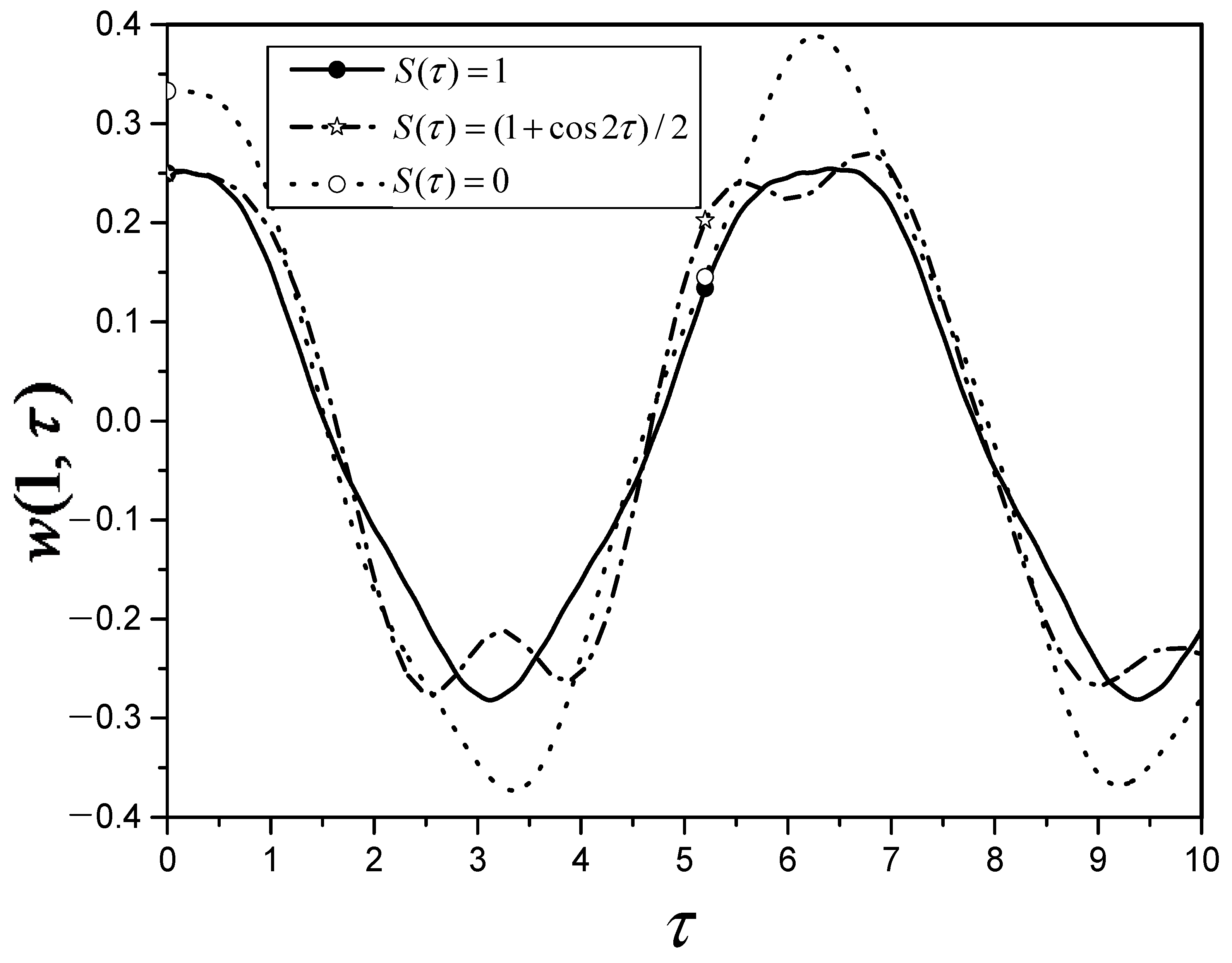
The deflection of the cantilever beam with a time-dependent spring support is between the two extreme cases of a pure cantilever beam and a cantilever beam with a constant spring coefficient.
(3)
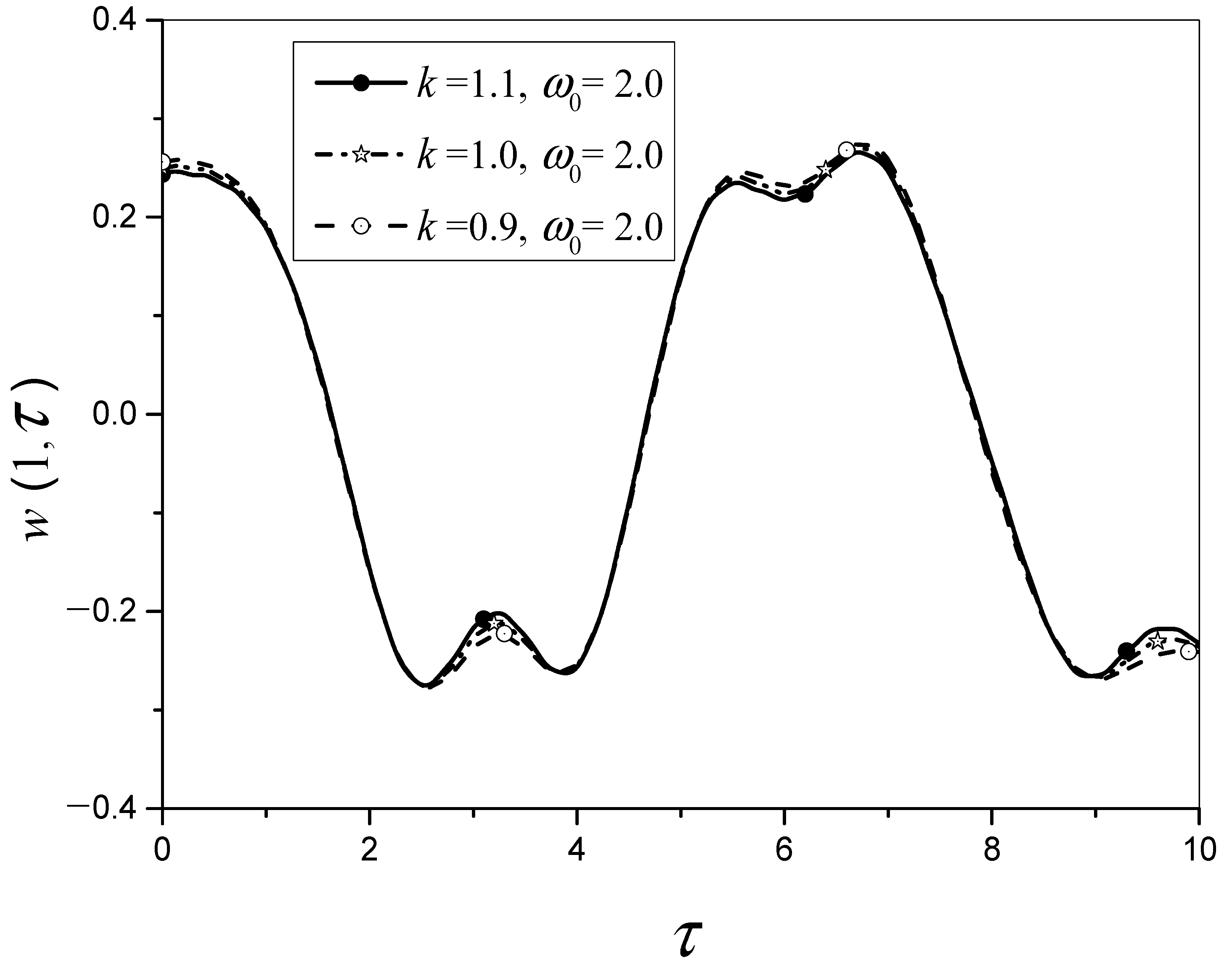
In the sensitivity analysis, the error in the spring frequency has a greater effect on the variation in the cantilever deflection than that in the spring magnitude.
(4)
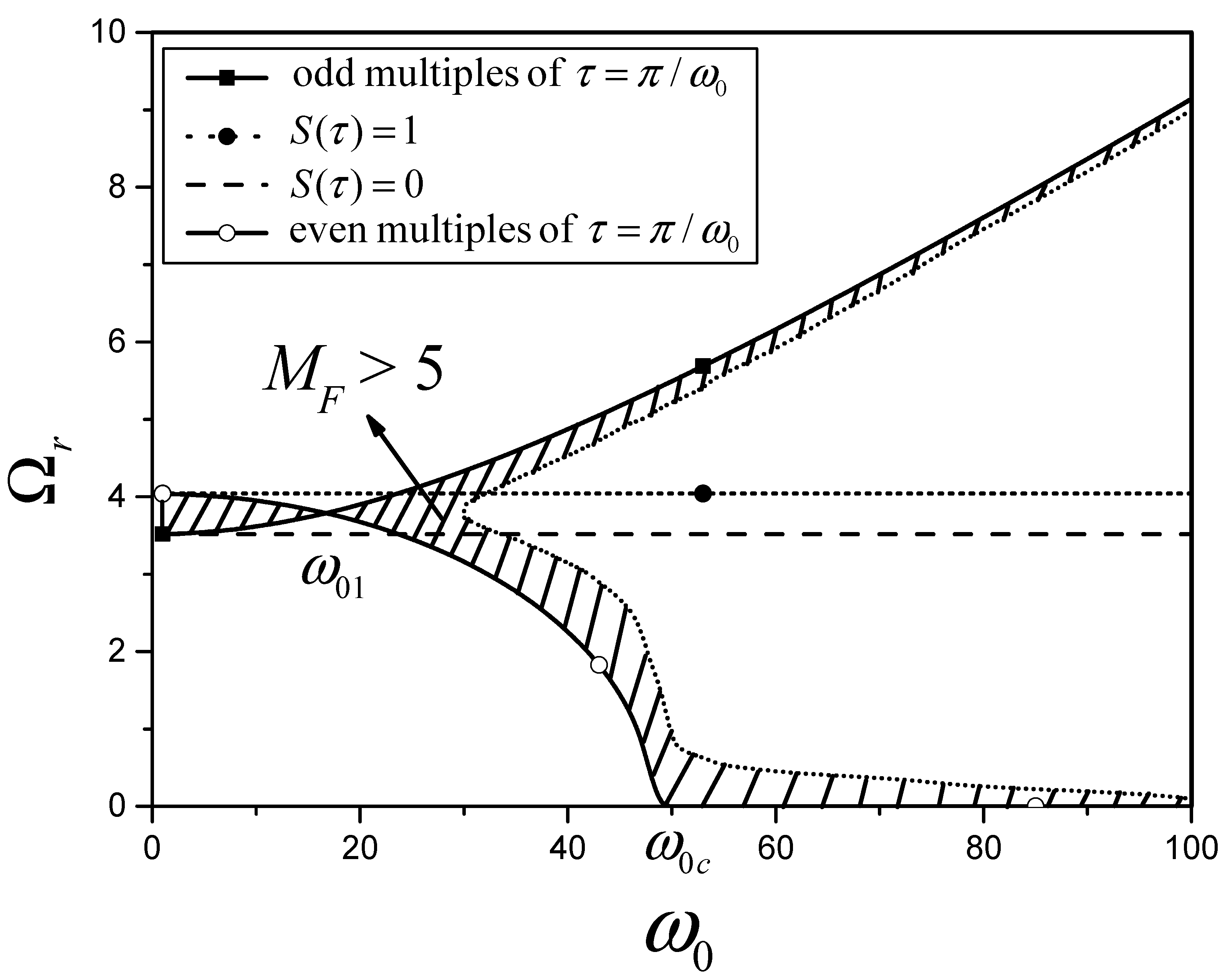
When the magnitude or the frequency of the spring stiffness is greater than a critical value, the divergence instability occurs in the first mode at even multiples of τ = π / ω 0 .
(5)
The important new finding is that the resonance frequency depends significantly on the magnitude and the frequency of the spring-like actuator in the first two modes. The magnitude and/or the frequency of the time-dependent spring stiffness can be adjusted to distribute the first two modes to avoid causing unsafe vibrations or even resonances of the beam system.
The resonance frequencies calculated using the proposed method were verified via a comparison with the exact solutions and with the solutions obtained using the separation of variables method in the extreme cases. However, it is also recommended that future work validate the results via a comparison with numerical and/or experimental data.

Author Contributions

Conceptualization, J.-R.C.; data curation, J.-R.C. and C.-J.H.; formal analysis, J.-R.C.; funding acquisition, J.-R.C.; investigation, J.-R.C., T.-W.T. and C.-J.H.; methodology, J.-R.C. and T.-W.T.; resources, T.-W.T.; software, J.-R.C. and C.-J.H.; supervision, T.-W.T.; validation, J.-R.C. and T.-W.T.; writing—original draft, C.-J.H.; writing—review and editing, J.-R.C. All authors have read and agreed to the published version of the manuscript.

Funding

This research received no external funding. Additionally, the APC was funded by all authors.

Data Availability Statement

Not applicable.

Conflicts of Interest

The authors declare no conflict of interest.

Nomenclature

A Cross-sectional area ( m 2 )
E Young’s modulus ( N / m 2 )
f Auxiliary function
g Shifting function
H n Auxiliary function
I Area moment of inertia ( m 4 )
k A constant spring stiffness magnitude
K Time-dependent spring stiffness ( N / m )
L Length of beam ( m )
M F Magnification factor
p Dimensionless forcing term
q n Time-dependent generalized coordinate
Q n Amplitude of q n
S Time-dependent spring function
tTime variable ( sec )
T n Phase angle of q n
v Transformed function
w Dimensionless flexural displacement of beam
w 0 ,   w ¯ 0 Dimensionless initial displacement and initial velocity
W Flexural displacement of beam
W 0 ,   W ¯ 0 Initial displacement and initial velocity
x Longitudinal coordinate of the beam ( m )

Greek Symbols

α A unit dimensionless time-dependent spring stiffness function
β n Auxiliary function
δ Delta function used in Equation (58)
δ n Auxiliary function
δ m n Kronecker delta
ϕ n Eigenfunction
ϕ n o r Norm of eigenfuction
φ Auxiliary integration variable
γ n , η n , κ n Auxiliary functions
λ n , λ ¯ n Characteristic values
τ Dimensionless time variable
ω 0 Frequency of time-dependent spring stiffness
ω 0 c Critical spring stiffness frequency
Frequency in forcing term
ξ Dimensionless coordinate
ζ n Auxiliary function

References

  1. Jia, X.L.; Ke, L.L.; Feng, C.B.; Yang, J.; Kitipornchai, S. Size effect on the free vibration of geometrically nonlinear functionally graded micro-beams under electrical actuation and temperature change. Compos. Struct. 2015, 133, 1137–1148. [Google Scholar] [CrossRef]
  2. Zhang, B.; Sui, Y.; Bu, Q.; He, X. Remaining useful life estimation for micro switches of railway vehicles. Control Eng. Pract. 2019, 84, 82–91. [Google Scholar] [CrossRef]
  3. Scornec, J.L.; Guiffarda, B.; Sevenoa, R.; Cam, V.L. Frequency tunable, flexible and low cost piezoelectric micro-generator for energy harvesting. Sens. Actuators A Phys. 2020, 312, 112148. [Google Scholar] [CrossRef]
  4. Wang, T.; Zhu, Z.-W. A new type of piezoelectric self-excited vibration energy harvester for micro-actuator’s energy storage. J. Energy Storage 2022, 46, 103519. [Google Scholar] [CrossRef]
  5. Wang, H.; Yamada, S.; Tanaka, S. Moving coil type electromagnetic microactuator using metal/silicon driving springs and parylene connecting beams for pure in-plane large motion in three axes. Sens. Actuators A Phys. 2022, 342, 113606. [Google Scholar] [CrossRef]
  6. Xie, Y.; Lei, J.; Guo, S.; Han, S.; Ruan, J.; He, Y. Size-dependent vibration of multi-scale sandwich micro-beams: An experimental study and theoretical analysis. Thin Walled Struct. 2022, 175, 109115. [Google Scholar] [CrossRef]
  7. Onoda, J.; Watanabe, N. Vibration suppression by variable-stiffness members. AIAA J. 1991, 29, 977–983. [Google Scholar] [CrossRef]
  8. Giirdal, Z.; Olmedo, R. In-plane response of laminates with spatially varying fiber orientations: Variable stiffness concept. AIAA J. 1993, 31, 751–758. [Google Scholar] [CrossRef]
  9. Kuder, I.K.; Arrieta, A.F.; Raither, W.E.; Ermanni, P. Variable stiffness material and structural concepts for morphing applications. Prog. Aerosp. Sci. 2013, 63, 33–55. [Google Scholar] [CrossRef]
  10. Sun, S.; Yang, J.; Li, W.; Deng, H.; Du, H.; Alici, G. Development of a novel variable stiffness and damping magnetorheological fluid damper. Smart Mater. Struct. 2015, 24, 085021. [Google Scholar] [CrossRef]
  11. Kumar, D.; Sarangi, S. Variable stiffness modeling of smart cantilever beam under the electrical loading condition. Procedia Comput. Sci. 2018, 133, 697–702. [Google Scholar] [CrossRef]
  12. Zhao, Y.; Meng, G. A bio-inspired semi-active vibration isolator with variable-stiffness dielectric elastomer: Design and modeling. J. Sound Vib. 2020, 485, 115592. [Google Scholar] [CrossRef]
  13. Baniasadi, M.; Foyouzat, A.; Baghani, M. Multiple shape memory effect for smart helical springs with variable stiffness over time and temperature. Int. J. Mech. Sci. 2020, 182, 105742. [Google Scholar] [CrossRef]
  14. Balachandran, B.; Magrab, E.B. Vibrations; Cambridge University Press: New York, NY, USA, 2018; Chapter 9; pp. 547–565. [Google Scholar]
  15. Meirovitch, L. Analytical Methods in Vibrations; The Macmillan Company: London, UK, 1967; Chapter 7; pp. 300–308. [Google Scholar]
  16. Nothmann, G.A. Vibration of a cantilever beam with prescribed end motion. ASME J. Appl. Mech. 1948, 15, 327–334. [Google Scholar] [CrossRef]
  17. Lee, S.Y.; Yan, Q.Z. An analytical solution for out-of-plane deflection of a curved Timoshenko beam with strong nonlinear boundary conditions. Acta Mech. 2015, 226, 3679–3694. [Google Scholar] [CrossRef]
  18. Yen, T.C.; Kao, S. Vibration of beam-mass systems with time-dependent boundary conditions. ASME J. Appl. Mech. 1959, 26, 353–356. [Google Scholar] [CrossRef]
  19. Mindlin, R.D.; Goodman, L.E. Beam vibrations with time-dependent boundary conditions. ASME J. Appl. Mech. 1950, 17, 377–380. [Google Scholar] [CrossRef]
  20. Edstrom, C.R. The vibrating beam with nonhomogeneous conditions. ASME J. Appl. Mech. 1981, 48, 669–670. [Google Scholar] [CrossRef]
  21. Grant, D.A. Beam vibrations with time-dependent boundary conditions. J. Sound Vib. 1983, 89, 519–522. [Google Scholar] [CrossRef]
  22. Herrmann, G. Forced motions of Timoshenko beam theory. ASME J. Appl. Mech. 1955, 22, 53–56. [Google Scholar] [CrossRef]
  23. Berry, J.G. and Nagdhi, On the vibration of elastic bodies having time-dependent boundary conditions. Q. Appl. Math. 1956, 14, 43–50. [Google Scholar] [CrossRef]
  24. Epstein, H.I. Vibrations with time-dependent internal conditions. J. Sound Vib. 1975, 39, 297–303. [Google Scholar] [CrossRef]
  25. Aravamudan, K.S.; Murthy, P.N. Nonlinear vibration of beams with time-dependent boundary conditions. Int. J. Nonlinear Mech. 1973, 8, 195–212. [Google Scholar] [CrossRef]
  26. Lee, S.Y.; Lin, S.M. Dynamic analysis of nonuniform beams with time-dependent elastic boundary conditions. ASME J. Appl. Mech. 1996, 63, 474–478. [Google Scholar] [CrossRef]
  27. Lee, S.Y.; Lin, S.M. Nonuniform Timoshenko beams with time-dependent elastic boundary conditions. J. Sound Vib. 1998, 217, 223–238. [Google Scholar] [CrossRef]
  28. Lin, S.M.; Lee, S.Y. The forced vibration and boundary control of pretwisted Timoshenko beams with general time-dependent elastic boundary conditions. J. Sound Vib. 2002, 254, 69–90. [Google Scholar] [CrossRef]
  29. Lin, S.M. Pretwisted nonuniform beams with time-dependent elastic boundary conditions. Am. Inst. Aeronaut. Astronaut. J. 1998, 36, 1516–1523. [Google Scholar] [CrossRef]
  30. Lee, S.Y.; Wang, W.R.; Chen, T.Y. A general approach on the mechanical analysis of nonuniform beams with nonhomogeneous elastic boundary conditions. ASME J. Appl. Mech. 1998, 120, 164–169. [Google Scholar] [CrossRef]
  31. Sajjadi, M.; Pishkenari, H.N.; Vossoughi, G. On the nonlinear dynamics of trolling-mode AFM: Analytical solution using multiple time scales method. J. Sound Vib. 2018, 423, 263–286. [Google Scholar] [CrossRef]
  32. Horssen, W.T.V.; Wang, Y.; Cao, G. On solving wave equations on fixed bounded intervals involving Robin boundary conditions with time-dependent coefficients. J. Sound Vib. 2018, 424, 263–271. [Google Scholar] [CrossRef]
  33. Ahmad, M.; Ansari, R.; Darvizeh, M. Free and forced vibrations of atomic force microscope piezoelectric cantilevers considering tip-sample nonlinear interactions. Thin Walled Struct. 2019, 145, 106382. [Google Scholar] [CrossRef]
  34. Wang, J.; Horssen, W.T.V.; Wang, J.-M. On resonances in transversally vibrating strings induced by an external force and a time-dependent coefficient in a Robin boundary condition. J. Sound Vib. 2021, 512, 116356. [Google Scholar] [CrossRef]
  35. Wang, X.; Meng, L.; Yao, Y.; Li, H. A vibration-driven locomotion robot excited by time-varying stiffness. Int. J. Mech. Sci. 2023, 243, 108009. [Google Scholar] [CrossRef]
Figure 1. Vibration of a cantilever beam with a novel spring-like actuator at the free end, subjected to a transverse load.
Axioms 12 00500 g001
Figure 2. Vibration of a cantilever beam with a time-dependent spring support at the free end, subjected to a transverse load.
Axioms 12 00500 g002
Figure 3. The deflection at the free end of a pure cantilever beam ( S ( τ ) = 0 ), a cantilever beam with a constant spring coefficient ( S ( τ ) = 1 ), and a cantilever beam with a time-dependent spring support ( S ( τ ) = ( 1 + cos 2 τ ) / 2 ).
Axioms 12 00500 g003
Figure 4. The deflection at the free end of a cantilever beam with a time-dependent spring support ( S ( τ ) = k α ( τ ) = k ( 1 + cos ω 0 τ 2 ) , ω 0 = 2 ).
Axioms 12 00500 g004
Figure 5. The deflection at the free end of a cantilever beam with a time-dependent spring support ( S ( τ ) = k ( 1 + cos ω 0 τ 2 ) , k = 1 ).
Axioms 12 00500 g005
Figure 6. The magnification factor of the first mode for the resonance frequency at eight different time points. [ k = 1 , ω 0 = 1 ].
Axioms 12 00500 g006
Figure 7. The relationship of the resonance frequency and the spring stiffness frequency for the first four modes at k = 1 .
Axioms 12 00500 g007
Figure 8. The relationship of the resonance frequency and the spring stiffness magnitude for the first four modes at ω 0 = 30 .
Axioms 12 00500 g008
Figure 9. Zoomed-in plot of the resonance frequency versus the spring stiffness frequency for the first mode at k = 1 .
Axioms 12 00500 g009
Figure 10. Zoomed-in plot of the resonance frequency versus the spring stiffness magnitude for the first mode at ω 0 = 30 .
Axioms 12 00500 g010
Table 1. The deflections of the beam at ξ = 1 and various time τ [ w 0 ( ξ ) = ξ 3 + 3 ξ 2 2 ( k + 3 ) , w ¯ 0 ( ξ ) = 0 , S ( τ ) = k = 1 , Ω = 1 ].
τ w   ( 1 ,   τ )
1 Term2 Terms3 Terms4 Terms5 Terms
ABABABABAB
00.23930.24020.24550.24850.24630.24950.24650.24980.24660.2499
10.15070.1480.15720.15250.15770.15310.15780.15320.15780.1533
2−0.1032−0.1030−0.1086−0.1064−0.1089−0.1069−0.1089−0.1070−0.1089−0.1070
3−0.2716−0.2674−0.2780−0.2756−0.2788−0.2767−0.2790−0.2770−0.2791−0.2771
4−0.1508−0.1531−0.1590−0.1586−0.1596−0.1593−0.1598−0.1594−0.1599−0.1595
50.06890.06920.07280.07150.07290.07180.0730.07190.0730.0719
60.2360.23580.24260.24380.24330.24480.24370.24510.24380.2452
70.21270.20860.22010.21480.22090.21560.22110.21580.22120.2159
8−0.0491−0.0469−0.0513−0.0481−0.0512−0.0483−0.0513−0.0483−0.0513−0.0483
9−0.2387−0.2367−0.2455−0.2443−0.2463−0.2453−0.2465−0.2455−0.2466−0.2456
10−0.1997−0.2005−0.2071−0.2075−0.2080−0.2083−0.2082−0.2086−0.2083−0.2087
A: Present solution, Equation (76); B: Separation of variables method, Equation (77).
Table 2. Convergence checks of the solutions of the proposed method in Table 1 under different numbers of expansion terms.
τ | A n + 1 A n A n + 1 |
n = 1 n = 2 n = 3 n = 4
02.53%0.325%0.0811%0.0376%
14.13%0.317%0.0634%0%
24.97%0.275%0%0%
32.30%0.287%0.0717%0.0358%
45.16%0.376%0.125%0.0625%
55.36%0.137%0.137%0%
62.72%0.288%0.164%0.0410%
73.36%0.362%0.0905%0.0452%
84.29%0.195%0.195%0%
92.77%0.325%0.0811%0.0406%
103.57%0.437%0.096%0.0480%
A n : Present solution with n terms expansion; A n + 1 : Present solution with n + 1 terms expansion.
Table 3. The sensitivity of the cantilever deflection with spring stiffness S ( τ ) = k ( 1 + cos ω 0 τ 2 ) for ω 0 = 2.0 , k = 1.0 , 0 τ 10 .
ParameterSensitivity
ω 0 = ω 0 , k = k s | Δ w ( 1 ,   τ ) Δ k | %  a
k s = 0.9 0.0463~13.5%
k s = 1.1 0.0566~13.1%
ω 0 = ω 0 s , k = k | Δ w ( 1 ,   τ ) Δ ω 0 | %  b
ω 0 s = 1.9 0.0~58.0%
ω 0 s = 2.1 0.0~63.9%
a: Δ w ( 1 ,   τ ) = w ( 1 ,   τ ) | ω 0 = ω 0 ,   k = k s w ( 1 ,   τ ) | ω 0 = ω 0 ,   k = k , Δ k = k k . b: Δ w ( 1 ,   τ ) = w ( 1 ,   τ ) | ω 0 = ω 0 s ,   k = k w ( 1 ,   τ ) | ω 0 = ω 0 ,   k = k , Δ ω 0 = ω 0 ω 0 .
Table 4. The resonance frequencies of various spring frequencies at various times for mode I and mode II [ k = 1 ].
ω 0 Mode IMode II
τ = π / ω 0 τ = 2 π / ω 0 τ = π / ω 0 τ = 2 π / ω 0
03.5164.03822.03422.126
(comparison)3.516
(ES a)
4.040
(SVM b)
22.034
(ES a)
22.126
(SVM b)
13.5174.03722.03422.126
23.5204.03522.03422.127
53.5414.01622.03122.130
103.6163.95022.02022.141
153.7373.83822.00122.160
203.9003.67421.97522.186
254.1003.45321.94222.219
304.3303.16121.90122.260
354.5912.77721.85322.308
404.8732.25421.79722.363
455.1741.44821.73422.426
475.2990.89821.70622.453
485.3630.37421.69222.467
a: Exact solution of the clamped-free beam system. b: Solution of the beam with constant spring stiffness by using separation of variables method.
Disclaimer/Publisher’s Note: The statements, opinions and data contained in all publications are solely those of the individual author(s) and contributor(s) and not of MDPI and/or the editor(s). MDPI and/or the editor(s) disclaim responsibility for any injury to people or property resulting from any ideas, methods, instructions or products referred to in the content.

