Article

Quasi-Magical Fermion Numbers and Thermal Many-Body Dynamics

by
Angelo Plastino
1,*,†,
Diana Monteoliva
2,† and
Angel Ricardo Plastino
3,†
1
Instituto de Física La Plata–CCT-CONICET, Universidad Nacional de La Plata, C.C. 727, La Plata 1900, Argentina
2
UNLP-Comisión de Investigaciones Científicas Provincia de Buenos Aires La Plata, La Plata 1900, Argentina
3
CeBio-Departamento de Ciencias Básicas, Universidad Nacional del Noroeste de la Prov. de Buenos Aires (UNNOBA), CONICET, Junin 6000, Argentina
*
Author to whom correspondence should be addressed.
These authors contributed equally to this work.
Axioms 2023, 12(5), 493; https://doi.org/10.3390/axioms12050493
Submission received: 4 April 2023 / Revised: 6 May 2023 / Accepted: 11 May 2023 / Published: 19 May 2023
(This article belongs to the Special Issue Advances in Quantum Theory and Quantum Computing)

Abstract

:
This work scrutinizes, using statistical mechanics indicators, important traits displayed by quantum many-body systems. Our statistical mechanics quantifiers are employed, in the context of Gibbs’ canonical ensemble at temperature T. A new quantifier of this sort is also presented here. The present discussion focuses attention on the role played by the fermion number N in many-fermion dynamics, that is, N is our protagonist. We have discovered discovers particular values of N for which the thermal indicators exhibit unexpected abrupt variations. Such a fact reflects an unanticipated characteristic of fermionic dynamics.

1. Introduction

Many-body quantum mechanics is used to study a wide range of physical systems, including solids, liquids, gases, and plasmas. It is particularly important in condensed matter physics, where it is used to study the behavior of large numbers of interacting electrons, and in nuclear physics, where it is used to study the properties of atomic nuclei.
There are many different approaches to solving the many-body problem, including mean field theory, perturbation theory, and Monte Carlo simulations. Each of these methods has its own strengths and weaknesses, and the choice of method often depends on the particular properties of the system being studied. One of the major challenges in many-body quantum mechanics is the so-called “curse of dimensionality”, which arises when the number of particles in the system becomes large. As the number of particles increases, the number of possible states of the system grows exponentially, making it difficult to solve the Schrödinger equation exactly. As a result, many approximations and numerical methods have been developed to study many-body quantum systems, for example, exactly solvable models, which have been studied here with a concentration on fermions.
In particular, many-fermion dynamics is the study of the behavior of systems consisting of multiple fermions, which are particles that obey the Pauli exclusion principle. Such systems can include atoms, molecules, and solids, as well as more exotic systems such as neutron stars and quark–gluon plasmas. The behavior of many-fermion systems is governed by the laws of quantum mechanics, which describe the probabilistic nature of the behavior of particles on the atomic and subatomic scales. In particular, the behavior of fermions is described by Fermi–Dirac statistics, which specify the probabilities of finding particles in different quantum states. Important tools for studying many-fermion dynamics are of course the many-body problem techniques, which involve calculating the behavior of a system of interacting particles. This problem is notoriously difficult, as it requires solving the Schrödinger equation for a system with a large number of particles. Many-fermion dynamics has important applications in many areas of physics, including condensed matter physics, nuclear physics, and astrophysics. By understanding the behavior of fermions in these systems, physicists can gain insights into the fundamental principles that govern the behavior of matter on the smallest scales.
As stated above, the quantum many-fermion system exhibits multiple features with surprising intricacy. Our study differs from others in the fact that we work at a finite temperature T using statistical mechanics. Thus, we will here try to investigate N-fermion-dependent traits employing the notion of statistical thermal order.
We have learnt a lot about the features of finite, quantum many-body systems thanks to new statistical tools derived from information theory, which have been used to analyze distinct aspects of the physics of (1) atoms, (2) molecules, and (3) atomic nuclei [1,2,3,4,5,6,7,8,9,10,11,12,13,14,15]. Accordingly, we use statistical quantifiers to generate insights into many fermion systems.
Exactly solvable models (ESM) are of great help in shedding light on these systems. In combination with information theoretical tools, ESM can yield useful insights into many body intricacies. We will apply here recent information theory techniques to exactly soluble many-fermion models of the Lipkin kind, a sort of Hubbard model [12]. Information-based works on many-body behavior at a finite temperature have indeed been found to be quite useful [13].
We remind the reader here that singular fermion numbers N s are known to exist in atomic nuclei, where they are called magic numbers. They occur as a consequence of the nuclear shell structure. The properties of a nucleus with nucleon number N s are quite different to those of nuclei with nucleon numbers close but different to N s . In more detail, people speak of some special numbers of protons or neutrons in a full shell as magic numbers N s , with N M = 2, 8, 20, 28, 50, 82, and 126. At these numbers, a shell becomes totally full, with particularly notable properties. Stability is the most important one. Here, we also will find stability not in a nuclear context but in a statistical mechanics context.

2. Statistical Notion of Order

In this paper, we try to link the notion of order to the dynamics of interacting fermions. As we shall see, our fermion systems are indeed endowed with order–disorder properties. These will be studied using Gibbs’ canonical ensemble methodology [16], in which entropy is denoted as S. In this methodology, the pertinent probability distribution (PD) is proportional to exp ( β H ^ ) , where H ^ stands of course for the Hamiltonian, while β stands for the inverse temperature. Maximal statistical disorder is usually associated with a uniform distribution (UD), since in this state, all micro-states are equiprobable. In contrast, maximal order is associated with systems for which just a very small set of micro-states display non vanishing probabilities.
We call disequilibrium, D, the distance (in probability space) between the current probability distribution (PD) and a UD. The quantity D is a statistical quantifier that grows as the degree of order increases, while at the same time the entropy S decreases. The product D S is called the statistical complexity [17]. Thus, a small D indicates disorder and a large D indicates order.

3. SU2-Based Fermion Models

Lipkin-like models can be regarded as non trivial, finite, exactly solvable, and easy to manage many-fermion systems [14,15]. Having such properties, these models are formidable grounds for devising new many-body techniques and testing them, since the new approximate methods can always be compared with the exact solution. Amongst these novel methodologies, we focus attention in this study to those taken from information theory. We try them on the Lipkin model and its relative the AFP model [18,19,20].

3.1. Lipkin Model

The Lipkin model consists of N = 2 Ω fermions distributed among ( 2 Ω )-fold degenerate single-particle (sp) levels. These two energy levels are characterized by an sp energy gap ϵ . We deal with 4 Ω sp micro-states and two degenerate energy levels. Two quantum numbers ( μ and p) are ascribed to a general sp micro-state. The first takes the values μ = 1 (lower level) and μ = + 1 (upper level). The other, called here p, is a quasi-spin or pseudo spin, and it singles out a specific micro-state belonging to the N-fold degeneracy. The couple p , μ is regarded as a “site” that is either occupied (by a fermion) or empty. Thus,
N = 2 J ,
where J is a kind of angular momentum. Lipkin et al. [14] use the so-called quasi-spin operators
J ^ + = p C p , + C p , ,
J ^ = p C p , C p , + ,
J ^ z = p , μ μ C p , μ C p , μ ,
J ^ 2 = J ^ z 2 + 1 2 ( J ^ + J ^ + J ^ J ^ + ) ,
where the eigenvalues of J ^ 2 are of the form J ( J + 1 ) . The Lipkin Hamiltonian reads [15] (V is the coupling constant that play a central role below):
H = ϵ J ^ z + ( V / 4 ) ( J ^ + 2 + J ^ 2 ) .

3.2. The AFP Model

For the AFP model, we have [18,19,20] a similar quasi-spin arrangement, which introduces the operators
G ^ i j = p = 1 2 Ω C p , i C p , j .
As above, we call V the coupling constant of the pertinent two-body interaction and regard it as the control parameter of the system. It plays an important role, the statistical reasoning for which is presented below. The Hamiltonian reads
H ^ A F P = ϵ i N G ^ i i + V ( J ^ x J ^ x 2 ) ,
where J ^ x is the well-known sum [ J ^ + + J ^ ] / 2 .

3.3. Hamiltonian Matrices

For the AFP, one deals (see Equation (6) in [19]) with the Hamiltonian matrix
n | H A F P | n = ( n J ) δ n , n + 1 2 V { 2 ( 2 J 2 + J + n 2 2 J n ) δ n , n + 2 ( 2 J n ) ( n + 1 ) δ n , n + 1 + 2 ( 2 J n + 1 ) n δ n , n 1 ( 2 J n 1 ) ( n + 2 ) ( 2 J n ) ( n + 1 ) δ n , n + 2 ( 2 J n + 2 ) ( n 1 ) ( 2 J n + 1 ) n δ n , n 2 .
For the Lipkin Hamiltonian, one has [15]
n | H L | n = N 2 n + 1 δ n , n V 2 ( N n ) ( N n + 1 ) ( n + 1 ) n δ n , n + 2 V 2 ( N n ) ( N n + 1 ) ( n + 1 ) n δ n , n 2 ,
where n = 0 , 1 , , N for J = N / 2 . Numerical diagonalization yields energy eigenvalues E n ( V , J ) for our two Hamiltonians. These eigenvalues are needed to build the partition function Z [16] in the canonical ensemble Z [16].

4. Statistical Mechanics Indicators

As we use statistical mechanics theory throughout, we need a special formalism that is provided in [21]. Statistical mechanics quantifiers are derived from the partition function Z [16] which one constructs employing probabilities linked to the microscopic states involved, whose energies are E i [16]. Important thermal indicators are (1) the mean energy U, (2) the entropy S, and (3) the free energy F [16]. They, together with Z, are obtained from the so-called canonical probability distributions [16] P n ( v , J β ) , with β being the inverse temperature. Note that J is intimately linked to N. The associated expressions are [16]
P n ( V , J , β ) = 1 Z ( V , J , β ) e β E n ( V , J )
Z ( V , J , β ) = n = 0 N e β E n ( V , J )
U ( V , J , β ) = E = l n Z ( V , J , β ) β = n = 0 N E n ( V , J ) P n ( v , J , β ) = 1 Z ( v , J , β ) n = 0 N E n ( V , J ) e β E n ( V , J )
S ( V , J , β ) = n = 0 N P n ( V , J , β ) ln [ P n ( V , J , β ) ]
F ( V , J , β ) = U ( V , J , β ) T S ( V , J , β ) .

Order Quantifiers

A special form of the order quantifiers was introduced about two and a half decades ago [17,22,23,24,25] (using Equations (11)–(15)). We refer to them here as specialized for the AFP–Lipkin models. We will place a strong emphasis on the so-called disequilibrium D A F P (quantities with sub-index L refer to the Lipkin model). For more details, see [21]. One deals with
D A F P ( v , J , β ) = n = 0 N P n A F P ( V , J , β ) P n u 2
D L ( v , J , β ) = n = 0 N P n L ( V , J , β ) P n u 2 .
Recall that our J-multiplets consist of N + 1 possible micro-states. Thus, the uniform distribution is
P n u = 1 N + 1 n = 0 , 1 , , N + 1 .
D is a Euclidean distance in probability space. Our disequilibrium D is an indicator of statistical order [17,22,23,24,25]. The bigger D is, the more it differs from P u . A value of D = 0 implies full randomization [17].
In addition, we appeal here to a novel thermal quantifier that resembles the one first introduced in [26]. This indicator measures how much work one needs to effect a change in the degree of order by varying N. In this sense, they may be used to assess thermal efficiency [26].
ν N = ( d D / d N ) / ( d F / d N ) ,
although, below, we often simplify ν N to just ν . The temperature T is regarded as fixed. N can take only discrete values. Thus, to give sense to derivatives with respect to N, one analytically extends the pertinent ranges to real values [27]. Here, we employ several interpolations sorts: (1) cubic polynomial interpolation, (2) Hermite polynomials, and (3) cubic splines [27]. In our graphs below, full curves represent interpolations, while dots represent exact results. Our ν s are, approximately, of the form Δ D ( δ N ) / Δ F ( δ N ) . Thus, the sign of ν depends on the interplay between the signs of the accompanying Δ s.
Note that the thermal quantifiers provide much more information than those available with just the quantum resources of zero temperature T. If we take a low enough T (a high enough β ), these indicators give a good idea of what happens when T vanishes. In what follows, we use the values of β = 20 , 30 , which should be high enough to indicate what happens when T vanishes.

5. Singular Values for the Fermion Numbers

We take the coupling constant V = 0.01 with β = 20 and plot F, S, D, and ν N vs. N. Remember that the system is variable, in which Δ F < 0 can occur in a spontaneous fashion. Thus, we pass now to consider the thermal behavior versus N in both Lipkin (Figure 1) and AFP (Figure 2) scenarios. The latter (AFP) results in a surprise. The AFP dynamics seem to abruptly change at N∼50, where F is at a minimum and shortly afterwards ceases to change as N grows. Thus, we might call N∼50 a kind of “singular number”. Starting with a low N, one realizes that the addition of fermions can spontaneously occur in the two models, favored by the F behavior ( F f i n a l F i n i t i a l = Δ F < 0 ). However, in the AFP scenario, the F values stabilize after a singular number is reached and then remain constant. Summing up, in the AFP instance (but not in the Lipkin one), F displays an abrupt behavior change at N∼50, where the system attains maximum stability because the free energy is at an absolute minimum there. To add or remove a fermion in such a situation requires work. Thus, our singular N value is associated with stability, as are the nuclear magic numbers.
Entropy describes information loss. Our next graphs (Figure 3 (AFP) and Figure 4 (Lipkin)) depict, without changing either V or β , the entropic behavior. Thus, one can assess the degree of information loss when N is varied. We see that for small values of N, the entropy is zero, which indicates that our system is represented by a nearly pure state (quantum pure states have zero entropy and maximum information). In the AFP case, this ceases to be true for N∼54, which enables us again to refer to singular numbers. A sudden loss of information occurs there. In the Lipkin case (Figure 4), near purity persists up to N∼100 and is then replaced by a mixed state of finite entropy (remember that for mixed states the entropy is not zero). Information loss can be said to take place for singular numbers near N = 100 . Accordingly, the entropic behavior is more complex in the Lipkin case (Figure 4). To repeat, for the Lipkin model, S vanishes for values smaller than N∼100 and then increases up to a constant finite value. Coming back to the AFP instance, we discover, putting together what happens with F, S, and D (see below), that its singular N value is associated with disordered stability.
We pass now to consider the disequilibrium D, a degree of order indicator. We have 0 D 1 . The larger D is, the larger the order degree. Here, we will find that information loss is associated with disorder growth, as one intuitively would presume. Figure 5 (AFP) and Figure 6 (Lipkin) depict the pertinent details. They are, of course, entirely in accordance with what one would expect after looking at the entropic results. If S is small, D must be large, and vice versa. In the AFP scenario, the order increases with the fermion number (slowly for most Ns) save for an abrupt fall at the singular number, where disorder increases, followed by a corresponding rapid ascent. The Lipkin scenario exhibits a rather more complicated picture. One observes a slow growth in D as N increases, until we reach the singular number (N∼100). Then, an abrupt descent (disorder grows) and stabilization at a much smaller order degree is observed.
Our final concern is related to our novel quantifier ν N ν , which is introduced in this work for the first time ever (we believe), inspired by the work in reference [26]. It measures the amount of work that should be instantiated by the system in order to produce a given order variation when N changes.
In the AFP scenario in Figure 7, ν N is zero until we reach the singular number. These values are obtained in a spontaneous fashion because a large amount of work is received by the system. For larger N values, ν slowly diminishes as N keeps growing.
In the Lipkin scenario in Figure 8, our quantifier ν N is negative for small N values, indicating that the system receives work to make the value of N increase. This entails (according to the definition of our quantifier) that the change in F is smaller than the associated D modification. ν vanishes at N∼25 for a while as N continues to increase, until we reach the singular number. In the pertinent N region, work should be done on the system to modify N, as ν is strongly positive at the singular N value of N∼100. Our indicator descends to zero afterwards as N keeps increasing, and there it indefinitely remains.
We demonstrate the same two graphs above in Figure 9 and Figure 10 for a lower temperature so as to confirm the results in Figure 7 and Figure 8.
Our quantifier ν behaves in a dramatically different fashion in our two SU2 models, which tells us how different the two associated fermion dynamics are.

6. Conclusions

We have investigated two different fermion dynamics generated by distinct exactly solvable Hamiltonians. We were interested in dynamical traits associated with the order–disorder disjunction. As we wanted to investigate situations closely related to those of the ground state, we used very low temperatures, which produced a reasonable approximation to what we wished to describe.
The subjects in which we are interested were clarified by appropriate statistical mechanics indicators. We studied the free energy, the entropy, the disequilibrium, and the disorder energy cost ν and their behavior when the number of fermions changes. The latter is a new quantifier introduced in the present work. These indicators were applied to two well-known fermion models called the AFP and Lipkin models. We ascertained just how the order–disorder disjunction was manifested in the models. The manifestation is of a quite different nature for each of the models. We observed very different dynamics, a fact that is not imaginable by just inspecting the two pertinent Hamiltonians.
A especially surprising result ensued, which was the emergence in the two models of special, singular fermion numbers, somewhat reminiscent of nuclear ones. The AFP singular N value signals stability, but the Lipkin one does not. Additionally, the determined singular number of fermion values indicates disorder growth. Our main point is indeed that the fermion dynamics suffer abrupt and remarkable changes at special N values that we called singular. Since this also happens for nuclei and electrons in atoms, one wonders if the existence of special N values is not a common characteristic of some fermion dynamical systems. More specifically:
  • The larger the value of N, the more stable the system becomes, as indicated by the behavior of the Lipkin free energy.
  • This is not so in the AGFO case, where there is an absolute free energy minimum at a specific “magic” number.
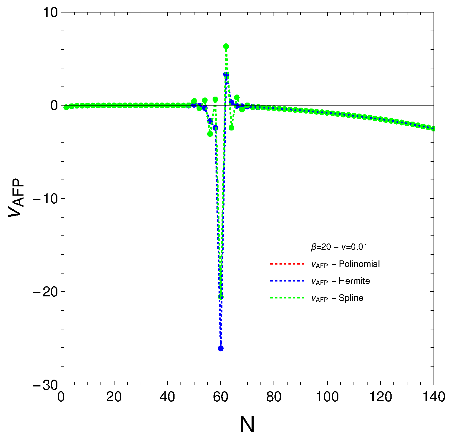
  • The main discovery with respect to the AFP entropy is the singular N value around N∼60 (the same as above). It signals not only stability but a loss of information.
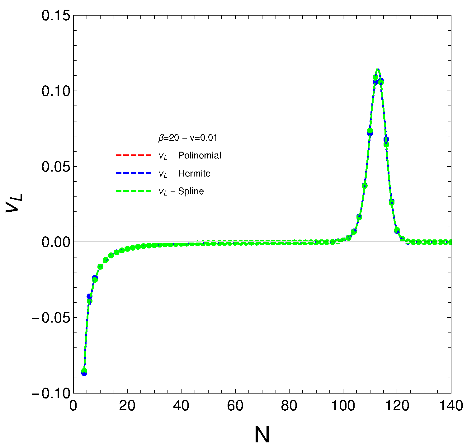
  • As regards Lipkin’s entropy, we have rather a lot to say. For small N numbers, the entropy almost vanishes, indicating a system in a mixed state close to the ground state. Then, and rather suddenly (magic number), as N grows, the system leaves the state described above and passes to a much more mixed state, losing information. The new state, however, remains stable as N continues to increase.
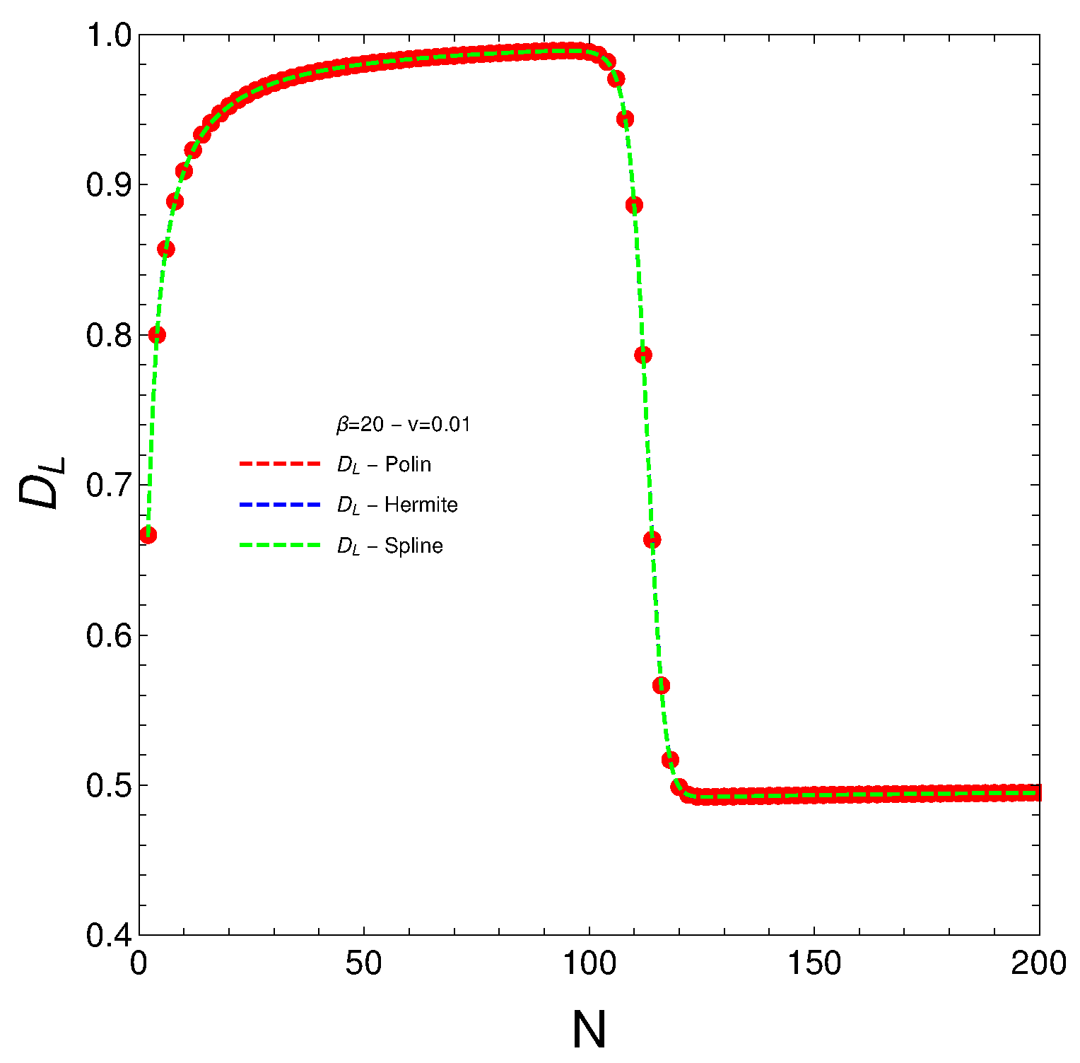
  • AFPs D. The degree of order is large, in general, as the system lies in a state close to the ground state, as we saw above. However, for the same quasi-magic number N as above, the system abandons that state, passing to a much more mixed state and losing “order” as a consequence. This situation reverts back to the original one as N keeps growing.
  • Lipkin’s D. The situation is much more complicated here than it was for the AFP model. For very small N values, this system lies in a disordered state. For moderate N values, a large degree of order is attained. Then, at the quasi-magic N value, the degree of order diminishes and then remains constant as N keeps increasing.

Author Contributions

All three authors participated in equal fashion in the research and planning of this paper. All authors have read and agreed to the published version of the manuscript.

Funding

This research received no external funding.

Data Availability Statement

Everything that might be needed is here.

Acknowledgments

We thank Conicet (Argentine Agency).

Conflicts of Interest

The authors declare no conflict of interest.

References

  1. Frank, R. Quantum criticality and population trapping of fermions by non-equilibrium lattice modulations. New J. Phys. 2013, 15, 123030. [Google Scholar] [CrossRef]
  2. Lubatsch, A.; Frank, R. Evolution of Floquet topological quantum states in driven semiconductors. Eur. Phys. J. B 2019, 92, 215. [Google Scholar] [CrossRef]
  3. Otero, D.; Proto, A.; Plastino, A. Surprisal Approach to Cold Fission Processes. Phys. Lett. 1981, 98, 225. [Google Scholar] [CrossRef]
  4. Satuła, W.; Dobaczewski, J.; Nazarewicz, W. Odd-Even Staggering of Nuclear Masses: Pairing or Shape Effect? Phys. Rev. Lett. 1998, 81, 3599. [Google Scholar] [CrossRef]
  5. Dugett, T.; Bonche, P.; Heenen, P.H.; Meyer, J. Pairing correlations. II. Microscopic analysis of odd-even mass staggering in nuclei. Phys. Rev. 2001, 65, 014311. [Google Scholar] [CrossRef]
  6. Ring, P.; Schuck, P. The Nuclear Many-Body Problem; Springer: Berlin, Germany, 1980. [Google Scholar]
  7. Uys, H.; Miller, H.G.; Khanna, F.C. Generalized statistics and high-Tc superconductivity. Phys. Lett. A 2001, 289, 264. [Google Scholar] [CrossRef]
  8. Kruse, M.K.G.; Miller, H.G.; Plastino, A.R.; Plastino, A.; Fujita, S. Landau-Ginzburg method applied to finite fermion systems: Pairing in nuclei. Eur. J. Phys. 2005, 25, 339. [Google Scholar] [CrossRef]
  9. de Llano, M.; Tolmachev, V.V. Multiple phases in a new statistical boson fermion model of superconductivity. Physical A 2003, 317, 546. [Google Scholar] [CrossRef]
  10. Xu, F.R.; Wyss, R.; Walker, P.M. Mean-field and blocking effects on odd-even mass differences and rotational motion of nuclei. Phys. Rev. C 1999, 60, 051301. [Google Scholar] [CrossRef]
  11. Häkkinen, H.; Kolehmainen, J.; Koskinen, M.; Lipas, P.O.; Manninen, M. Universal Shapes of Small Fermion Clusters. Phys. Rev. Lett. 1997, 78, 1034. [Google Scholar] [CrossRef]
  12. Hubbard, J. Electron Correlations in Narrow Energy Bands. Proc. R. Soc. Lond. 1963, 276, 237. [Google Scholar]
  13. Liu, Y. Exact solutions to nonlinear Schrodinger equation with variable coefficients. Appl. Math. Comput. 2011, 217, 5866. [Google Scholar] [CrossRef]
  14. Lipkin, H.J.; Meshkov, N.; Glick, A.J. Validity of many-body approximation methods for a solvable model: (I). Exact solutions and perturbation theory. Nucl. Phys. 1965, 62, 188. [Google Scholar] [CrossRef]
  15. Co, G.; Leo, S.D. Analytical and numerical analysis of the complete Lipkin–Meshkov–Glick Hamiltonian. Int. J. Mod. Phys. E 2018, 27, 5. [Google Scholar]
  16. Reif, F. Fundamentals of Statistical Theoretic and Thermal Physics; McGraw Hill: New York, NY, USA, 1965. [Google Scholar]
  17. López Ruiz, R.; Mancini, H.L.; Calbet, X. A statistical measure of complexity. Phys. Lett. A 1995, 209, 321. [Google Scholar] [CrossRef]
  18. Arrachea, L.; Canosa, N.; Plastino, A.; Portesi, M.; Rossignol, R. Maximum Entropy Approach Crit. Phenom. Finite Quantum Systems. Phys. Rev. A 1992, 45, 44. [Google Scholar] [CrossRef]
  19. Abecasis, S.M.; Faessler, A.; Plastino, A. Appl. Multi Config. Hartree-Fock Theory A SimpleModel. Z. Phys. 1969, 218, 394. [Google Scholar] [CrossRef]
  20. Feng, D.H.; Gilmore, R.G. Phase transitions in nuclear matter described by pseudospin Hamiltonians. Phys. Rev. C 1992, 26, 1244. [Google Scholar] [CrossRef]
  21. Plastino, A.R.; Monteoliva, D.; Plastino, A. Information-theoretic features of many fermion systems: An exploration based on exactly solvable models. Entropy 2021, 23, 1488. [Google Scholar] [CrossRef]
  22. López-Ruiz, R. A information-theoretic Measure of Complexity. In Concepts and Recent Advances in Generalized Information Measures and Statistics; Kowalski, A., Rossignoli, R., Curado, E.M.C., Eds.; Bentham Science Books: New York, NY, USA, 2013; pp. 147–168. [Google Scholar]
  23. Martin, M.T.; Plastino, A.; Rosso, O.A. Generalized information-theoretic complexity measures: Geometrical and analytical properties. Physica A 2006, 369, 439. [Google Scholar] [CrossRef]
  24. Dehesa, J.S.; López-Rosa, S.; Manzano, D. Configuration complexities of hydrogenic atoms. Eur. Phys. J. D 2009, 55, 539. [Google Scholar] [CrossRef]
  25. Esquivel, R.O.; Molina-Espiritu, M.; Angulo, J.C.J.; Antoín, J.; Flores-Gallegos, N.; Dehesa, J.S. Information-theoretical complexity for the hydrogenic abstraction reaction. Mol. Phys. 2011, 109, 2353. [Google Scholar] [CrossRef]
  26. Nigmatullin, R.; Prokopenko, M. Thermodynamic efficiency of interactions in self-organizing systems. Entropy 2021, 23, 757. [Google Scholar] [CrossRef] [PubMed]
  27. Humpherys, J.; Jarvis, J.T. Interpolation. Foundations of Applied Mathematics Volume 2: Algorithms, Approximation, Optimization; Society for Industrial and Applied Mathematics: Philadelphia, PA, USA, 2020. [Google Scholar]
Figure 1. Lipkin free energy F vs. N for V = 0.01 and β = 20 . V is a dimensionless variable and T is measured in Kelvins. The larger N is, the more stable the system becomes, as a low free energy is a sign of stability [16].
Axioms 12 00493 g001
Figure 2. AFP free energy F vs. N for V = 0.01 and β = 20 . V is a dimensionless variable and T is measured in Kelvins. Notice the minimum at N∼50 indicates maximal stability, as discussed in the text. Note that for the AFP model, things are quite different to the Lipkin case. This seems to show that a simple change in the fermion–fermion interaction form has a great effect on the free energy.
Axioms 12 00493 g002
Figure 3. AFP entropy S versus N for V = 0.01 and β = 20 . V is a dimensionless variable and T is measured in Kelvins. The main discovery here is the singular N value around N∼60. It signals a significant loss of information only for a very specific particle number, which we might call a quasi-magic number.
Axioms 12 00493 g003
Figure 4. Lipkin entropy S vs. N for V = 0.01 and β = 20 . V is a dimensionless variable and T is measured in Kelvins. Note that the precision of the curves is not too high. For small values of N, the entropy almost vanishes, indicating a system in a mixed state close to the ground state. Then, and rather suddenly as N grows, the system leaves the state described above and passes to a much more mixed state, losing information. The new state, however, remains stable as N continues to increase.
Axioms 12 00493 g004
Figure 5. AFP D vs. N for V = 0.01 and β = 20 . V is a dimensionless variable and T is measured in Kelvins. Remember that D measures order. This degree of order is large, in general, as the system lies in a state close to the ground state, as we saw above. However, for a quasi-magic number N, the system abandons that state, passing to a much more mixed one and losing “order” as a consequence. This situation reverts back to the original one as N keeps growing.
Axioms 12 00493 g005
Figure 6. Lipkin D vs. N for V = 0.01 and β = 20 . V is a dimensionless variable and T is measured in Kelvins. The situation is much more complicated here than it was for the AFP model. For very small values of N, this system lies in a disordered state. For moderate values of N, a large degree of order is attained. Then, at a quasi-magic N value, the degree of order diminishes and then remains constant as N keeps increasing.
Axioms 12 00493 g006
Figure 7. AFP ν versus N for V = 0.01 and β = 20 . V is a dimensionless variable and T is measured in Kelvins. Notice that around N = 60 , the energy cost ν abruptly becomes strongly negative, after being almost null for smaller values of N.
Axioms 12 00493 g007
Figure 8. Lipkin ν vs. N for V = 0.01 and β = 20 . V is a dimensionless variable and T is measured in Kelvins. The strong positive peak near N = 110 implies that work is done on the system to make the degree of order decrease.
Axioms 12 00493 g008
Figure 9. AFP ν versus N for V = 0.01 and β = 30 . V is a dimensionless variable and T is measured in Kelvins. Notice that around N = 60 , the energy cost ν abruptly becomes strongly negative, after being almost null for smaller values of N.
Axioms 12 00493 g009
Figure 10. Lipkin ν vs. N for V = 0.01 and β = 30 . V is a dimensionless variable and T is measured in Kelvins. The strong positive peak near N = 110 implies that work is done on the system to make the degree of order decrease.
Axioms 12 00493 g010
Disclaimer/Publisher’s Note: The statements, opinions and data contained in all publications are solely those of the individual author(s) and contributor(s) and not of MDPI and/or the editor(s). MDPI and/or the editor(s) disclaim responsibility for any injury to people or property resulting from any ideas, methods, instructions or products referred to in the content.

