Article

The Influence of White Noise and the Beta Derivative on the Solutions of the BBM Equation

by
Farah M. Al-Askar
1,
Clemente Cesarano
2 and
Wael W. Mohammed
3,4,*
1
Department of Mathematical Science, Collage of Science, Princess Nourah Bint Abdulrahman University, P.O. Box 84428, Riyadh 11671, Saudi Arabia
2
Section of Mathematics, International Telematic University Uninettuno, Corso Vittorio Emanuele II, 39, 00186 Roma, Italy
3
Department of Mathematics, Collage of Science, University of Ha’il, Ha’il 2440, Saudi Arabia
4
Department of Mathematics, Faculty of Science, Mansoura University, Mansoura 35516, Egypt
*
Author to whom correspondence should be addressed.
Axioms 2023, 12(5), 447; https://doi.org/10.3390/axioms12050447
Submission received: 10 April 2023 / Revised: 26 April 2023 / Accepted: 28 April 2023 / Published: 30 April 2023
(This article belongs to the Special Issue Special Topics in Differential Equations with Applications)

Abstract

:
In the current study, we investigate the stochastic Benjamin–Bona–Mahony equation with beta derivative (SBBME-BD). The considered stochastic term is the multiplicative noise in the Itô sense. By combining the F -expansion approach with two separate equations, such as the Riccati and elliptic equations, new hyperbolic, trigonometric, rational, and Jacobi elliptic solutions for SBBME-BD can be generated. The solutions to the Benjamin–Bona–Mahony equation are useful in understanding various scientific phenomena, including Rossby waves in spinning fluids and drift waves in plasma. Our results are presented using MATLAB, with numerous 3D and 2D figures illustrating the impacts of white noise and the beta derivative on the obtained solutions of SBBME-BD.
MSC:
35C08; 35C07; 35C05; 83C15; 35A20

1. Introduction

Nonlinear evolution equations (NEEs) are utilized to explain complex phenomena in many disciplines, including optical fiber communication, chemical kinetics, population dynamics, chaotic systems, photonic, plasma physics, electromagnetism, ocean wave, wave propagation, nuclear physics, fluid mechanics, and solid-state physics. Obtaining traveling wave solutions for NEEs is the most significant physical challenge. There are several effective methods for solving NEEs, including the generalized Kudryashov approach [1], modified decomposition approach [2], Riccati equation expansion [3], sine-Gordon expansion [4], sine-cosine method [5], Exp-function [6], improved tan ( φ / 2 ) -expansion [7], Lie symmetry [8], Jacobi elliptic function [9], and the tanh–sech method [10].
Recently, numerous mathematicians have introduced several fractional derivatives. Some of the most well-known are those presented by Caputo, Riemann-Liouville, Grunwald-Letnikov, Kober, Erdelyi, Marchaud, Hadamard, and Riesz [11,12,13,14]. Most kinds of fractional derivatives do not follow the chain rule, quotient rule, or product rule. In recent years, Atangana et al. [15] produced a new operator derivative called the beta-derivative (BD), which extends the classical derivative. If f : ( 0 , ) R then its beta derivative [15] is defined as:
D x β ϕ ( x ) = d β ϕ d x β = lim h 0 ϕ ( x + h ( x + 1 Γ ( β ) ) 1 β ) ϕ ( x ) h , 0 < β 1 .
Moreover, the BD possesses the following properties [15] for all real numbers a and b:
(1)
D x β f ( y ) = ( x + 1 Γ ( β ) ) 1 β d f d x ,
(2)
D x β ( a f + b g ) = a D x β ( f ) + b D x β ( g ) ,
(3)
D x β ( f g ( x ) ) = ( x + 1 Γ ( β ) ) 1 β g ( x ) f ( g ( x ) ) ,
(4)
D x β ( a ) = 0 .
Moreover, stochastic partial differential equations (SDEs) have a wide range of applications in physics, including molecular dynamics, neurodynamics, climate dynamics, geophysics, biology, physics, chemistry, and other scientific disciplines [16,17,18]. More precisely, SDEs characterize all dynamical equations in which quantum influences are either insignificant or can be accounted for as perturbations. SDEs are an extension of the theory of dynamical systems to models with noise. This is a significant generalization because actual systems cannot be entirely isolated from their surroundings and, as a result, are always subject to external stochastic influence.
As a consequence, obtaining exact solutions to fractional or stochastic differential equations is critical. Many analytical and numerical methods, including the ( G / G ) -expansion method [19], the mapping method [20], the Jacobi elliptic function technique [21], the extended tanh-coth method [22], bifurcation analysis [23,24], and more.
Therefore, it is critical here to look at the stochastic Benjamin–Bona–Mahony equation with beta derivative (SBBME-BD) as follows:
Q t + 6 QD x β Q + D x x x β Q α D x x β Q t = σ ( Q α D x x β Q ) B t ,
where the function Q = Q ( x , t ) is real, σ is the strength of the noise, B = B ( t ) is a white noise that satisfies the following properties: (i) B has continuous trajectories, (ii) B ( 0 ) = 0 , and (iii) B ( t i + 1 ) B ( t i ) has standard normal distribution. If we put σ = 0 , and β = 1 , then we obtain the Benjamin–Bona–Mahony equation as follows:
Q t + 6 QQ x + Q x x x α Q x x t = 0 .
Benjamin, Bona, and Mahony [25] investigated Equation (2) as a modification of the KdV equation. The modified equation was proposed to simulate long surface gravity waves with small amplitudes propagating in a 1 + 1 dimension. Many researchers have acquired the exact solutions of Equation (2) by applying many various methods, such as the generalized ( G / G )-expansion method [26], ( G / G )-expansion method [27], Hirota’s bilinear method [28], the Lie group method [29], the exp-function method [30], the tanh–coth method, and the sn–ns method [31]. The stochastic Benjamin–Bona–Mahony equation with beta derivative has not been considered until now.
The motivation behind this study is to obtain exact stochastic solutions of SBBME-BD (1) using the F -expansion approach combined with two distinct equations, namely the Riccati and elliptic equations. The presence of a stochastic term in the equation makes these solutions particularly useful for physicists in understanding important physical phenomena. Moreover, we present various 2D and 3D graphical representations using the MATLAB program to explore the impact of the Beta derivative and noise on the exact solution of SBBME-BD (1).
The sequence of the paper is as follows: In Section 2, we derive the wave equation for the SBBME-BD (1). In Section 3, the solution of the SBBME-BD (1) may be obtained by using F white noise and the BD on the obtained solutions of SBBME-BD (1). In the end, the conclusions of this paper are introduced.

2. Traveling Wave Equation for SBBME-BD

The wave equation for SBBME-BD (1) is achieved by applying:
Q ( x , t ) = G ( ζ ) e [ σ B ( t ) 1 2 σ 2 t ] , ζ = ζ 1 β ( x + 1 Γ ( β ) ) β + ζ 2 t ,
where G is a deterministic function, and ζ 1 , ζ 2 are unknown constants. We note that
Q t = [ ζ 2 G + σ GB t + 1 2 σ 2 G 1 2 σ 2 G ] e [ σ B ( t ) 1 2 σ 2 t ] = [ ζ 2 G + σ GB t ] e [ σ B ( t ) 1 2 σ 2 t ] ,
and
D x x β Q t = [ ζ 1 2 ζ 2 G + σ ζ 1 2 G B t ] e [ σ B ( t ) 1 2 σ 2 t ]
D x β Q = ζ 1 G e [ σ B ( t ) 1 2 σ 2 t ] , D x x x β Q = ζ 1 3 G e [ σ B ( t ) 1 2 σ 2 t ] .
Inserting Equation (3) into Equation (1) and utilizing (4)–(6), we obtain
ζ 2 G + ( ζ 1 3 α ζ 1 2 ζ 2 ) G + 6 ζ 1 GG e [ σ B ( t ) 1 2 σ 2 t ] = 0 .
Taking the expectations on both sides, we have
ζ 2 G + ( ζ 1 3 α ζ 1 2 ζ 2 ) G + 6 ζ 1 GG e 1 2 σ 2 t E e [ σ B ( t ) ] = 0 .
Since B ( t ) is a Gaussian process, then E ( e σ B ( t ) ) = e 1 2 σ 2 t . Thus, Equation (8) becomes
ζ 2 G + ( ζ 1 3 α ζ 1 2 ζ 2 ) G + 6 ζ 1 GG = 0 .
Integrating Equation (9) once with a zero integration constant yields
G + γ 1 G + γ 2 G 2 = 0 ,
where
γ 1 = ζ 2 ( ζ 1 3 α ζ 1 2 ζ 2 ) and γ 2 = 3 ( ζ 1 2 α ζ 1 ζ 2 ) .

3. Exact Solutions of SBBME-BD

Utilizing the F -expansion method ( F -EM) with two different equations, such as the Riccati equation and elliptic equation, the solutions to Equation (10) are discovered. Afterward, the SBBME-BD solutions (1) can be obtained.

3.1. F -EM with Riccati Equation

Assuming that the solution G of Equation (10) has the form:
G ( ζ ) = 0 + k = 1 J k F k ,
where F is the solution of the Riccati equation:
F = F 2 + ϕ ,
Determining J needs balancing G with G 2 in Equation (10) as
J + 2 = 2 J J = 2 .
Equation (11) becomes
G ( ζ ) = 0 + 1 F + 2 F 2 .
Equation (12) has the following solution:
F ( ζ ) = ϕ tan ( ϕ ζ ) or F ( ζ ) = ϕ cot ( ϕ ζ ) ,
If ϕ > 0 , or
F ( ζ ) = ϕ tanh ( ϕ ζ ) or F ( ζ ) = ϕ coth ( ϕ ζ ) ,
If ϕ < 0 , or
φ ( ζ ) = 1 ζ ,
If ϕ = 0 .
Now, putting Equation (13) into Equation (10), we have
( 6 2 + γ 2 2 2 ) F 4 + ( 2 1 + 2 γ 2 1 2 ) F 3 + ( 8 ϕ 2 + 2 0 2 γ 2 + 1 2 γ 2 + γ 1 2 ) F 2 ( 2 ϕ 1 + γ 1 1 + 2 γ 2 0 1 ) F + ( 2 ϕ 2 2 + γ 1 0 + γ 2 0 2 ) = 0
Putting the coefficients of F to zero:
6 2 + γ 2 2 2 = 0 ,
2 1 + 2 γ 2 1 2 = 0 ,
8 ϕ 2 + 2 0 2 γ 2 + 1 2 γ 2 + γ 1 2 = 0 ,
2 ϕ 1 + γ 1 1 + 2 γ 2 0 1 = 0 ,
and
2 ϕ 2 2 + γ 1 0 + γ 2 0 2 = 0 .
By solving these equations, we obtain the two families of solutions:
First family:
0 = 6 ϕ γ 2 , 1 = 0 , 2 = 6 γ 2 , ζ 2 = 4 ϕ ζ 1 3 1 + 4 α ϕ ζ 1 2 ,
Second family:
0 = 2 ϕ γ 2 , 1 = 0 , 2 = 6 γ 2 , ζ 2 = 4 ϕ ζ 1 3 1 4 α ϕ ζ 1 2 ,
First family: The solution to Equation (10) is as follows:
G ( ζ ) = 6 ϕ γ 2 6 γ 2 F 2 ( ζ ) .
There are three distinct cases for F ( ζ ) :
Case 1: If ϕ > 0 , then with (14), we have
G ( ζ ) = 6 ϕ γ 2 6 ϕ γ 2 tan 2 ( ϕ ζ ) = 6 ϕ γ 2 sec 2 ( ϕ ζ ) ,
and
G ( ζ ) = 6 ϕ γ 2 6 ϕ γ 2 cot 2 ( ϕ ζ ) = 6 ϕ γ 2 csc 2 ( ϕ ζ ) .
Consequently, the solution of SBBME-BD (1) is
Q ( x , t ) = 6 ϕ γ 2 sec 2 ( ϕ ζ ) e ( σ B ( t ) 1 2 σ 2 t ) ,
and
Q ( x , t ) = 6 ϕ γ 2 csc 2 ( ϕ ζ ) e ( σ B ( t ) 1 2 σ 2 t ) ,
where ζ = ζ 1 β ( x + 1 Γ ( β ) ) β + 4 ϕ ζ 1 3 1 + 4 α ϕ ζ 1 2 t .
Case 2: If ϕ < 0 , then by using (15), we have
G ( ζ ) = 6 ϕ γ 2 + 6 ϕ γ 2 tanh 2 ( ϕ ζ ) = 6 ϕ γ 2 sec h 2 ( ϕ ζ ) ,
and
G ( ζ ) = 6 ϕ γ 2 + 6 ϕ γ 2 coth 2 ( ϕ ζ ) = 6 ϕ γ 2 csc h 2 ( ϕ ζ ) .
Consequently, the solution of SBBME-BD (1) is
Q ( x , t ) = 6 ϕ γ 2 sec h 2 ( ϕ ζ ) e ( σ B ( t ) 1 2 σ 2 t ) ,
and
Q ( x , t ) = 6 ϕ γ 2 csc h 2 ( ϕ ζ ) e ( σ B ( t ) 1 2 σ 2 t ) .
Case 3: If ϕ = 0 , then by using (16), we have
G ( ζ ) = 6 γ 2 1 ζ 2 .
Consequently, the solution of SBBME-BD (1) is
Q ( x , t ) = [ 6 γ 2 1 ζ 2 ] e ( σ B ( t ) 1 2 σ 2 t ) ,
where ζ = ζ 1 β ( x + 1 Γ ( β ) ) β + 4 ϕ ζ 1 3 1 + 4 α ϕ ζ 1 2 t .
Second family: Equation (10) has the solution
G ( ζ ) = 2 ϕ γ 2 6 γ 2 F 2 ( ζ )
There are three distinct cases for F ( ζ ) :
Case 1: If ϕ > 0 , then by using (14), we have
G ( ζ ) = 2 ϕ γ 2 6 ϕ γ 2 tan 2 ( ϕ ζ ) ,
and
G ( ζ ) = 2 ϕ γ 2 6 ϕ γ 2 cot 2 ( ϕ ζ ) .
Consequently, the solution of SBBME-BD (1) is
Q ( x , t ) = [ 2 ϕ γ 2 6 ϕ γ 2 tan 2 ( ϕ ζ ) ] e ( σ B ( t ) 1 2 σ 2 t ) ,
and
Q ( x , t ) = [ 2 ϕ γ 2 6 ϕ γ 2 cot 2 ( ϕ ζ ) ] e ( σ B ( t ) 1 2 σ 2 t ) ,
where ζ = ζ 1 β ( x + 1 Γ ( β ) ) β 4 ϕ ζ 1 3 1 4 α ϕ ζ 1 2 t .
Case 2: If ϕ < 0 , then by using (15), we have
G ( ζ ) = 2 ϕ γ 2 + 6 ϕ γ 2 tanh 2 ( ϕ ζ ) ,
and
G ( ζ ) = 2 ϕ γ 2 + 6 ϕ γ 2 coth 2 ( ϕ ζ ) .
Consequently, the solution of SBBME-BD (1) is
Q ( x , t ) = [ 2 ϕ γ 2 + 6 ϕ γ 2 tanh 2 ( ϕ ζ ) ] e ( σ B ( t ) 1 2 σ 2 t ) ,
and
Q ( x , t ) = [ 2 ϕ γ 2 + 6 ϕ γ 2 coth 2 ( ϕ ζ ) ] e ( σ B ( t ) 1 2 σ 2 t ) ,
where ζ = ζ 1 β ( x + 1 Γ ( β ) ) β 4 ϕ ζ 1 3 1 4 α ϕ ζ 1 2 t .
Case 3: If ϕ = 0 , then by using (16), we have
G ( ζ ) = 6 γ 2 1 ζ 2 .
Consequently, the solution of SBBME-BD (1) is
Q ( x , t ) = 6 γ 2 1 ζ 2 e ( σ B ( t ) 1 2 σ 2 t ) ,
where ζ = ζ 1 β ( x + 1 Γ ( β ) ) β 4 ϕ ζ 1 3 1 4 α ϕ ζ 1 2 t .

3.2. F -EM with Elliptic Equation

Suppose that the solution of Equation (10) has the form (13). However, at this time, F solves the following elliptic equation:
F = R + K F 2 + P F 4 ,
where R , K , and P are constants. Differentiating Equation (13) twice and using (29), we have
G = 1 ( K F + 2 P F 3 ) + 2 2 ( R + 2 K F 2 + 3 P F 4 ) .
Setting Equations (13) and (30) into Equation (10), we have
( 6 2 P + γ 2 2 2 ) F 4 + ( 2 P 1 + 2 1 2 γ 2 ) F 3 + ( 4 2 K + 2 γ 2 0 2 + 1 2
+ 2 γ 1 ) F 2 + ( 1 K + 2 γ 2 0 1 + γ 1 1 ) F + ( 2 R 2 + γ 1 0 + γ 2 0 2 ) = 0 .
If we assign each coefficient of F k to 0, we will have a system of equations. Here are the two families we obtain when we solve this system for K 2 3 R P > 0 :
First family:
0 = 2 ( K + ( K 2 3 R P ) γ 2 ) , 1 = 0 , 2 = 6 P γ 2 , ζ 2 = 4 ( K 2 3 R P ) ζ 1 3 1 + 4 α ( K 2 3 R P ) ζ 1 2 .
Second family:
0 = 2 ( K ( K 2 3 R P ) γ 2 ) , 1 = 0 , 2 = 6 P γ 2 , ζ 2 = 4 ( K 2 3 R P ) ζ 1 3 1 4 α ( K 2 3 R P ) ζ 1 2 .
In both families, the solution of Equation (10) takes the form:
G ( ζ ) = 0 + 2 F 2 ( ζ ) .
There are many cases for F depending on P , K and R such that K 2 3 R P > 0 as follows:
CasePKR F ( ζ )
1 ρ 2 ( 1 + ρ 2 ) 1 s n ( ζ )
21 2 ρ 2 1 ρ 2 ( 1 ρ 2 ) d s ( ζ )
31 2 ρ 2 ( 1 ρ 2 ) c s ( ζ )
4 ρ 2 2 ρ 2 1 ( 1 ρ 2 ) c n ( ζ )
5 1 2 ρ 2 ( ρ 2 1 ) d n ( ζ )
6 ρ 2 4 ( ρ 2 2 ) 2 1 4 ( or ρ 2 4 ) s n ( ζ ) 1 ± d n ( ζ )
7 1 4 ( ρ 2 + 1 ) 2 ( 1 ρ 2 ) 2 4 ρ c n ( ζ ) ± d n ( ζ )
8 ρ 2 1 4 ( ρ 2 + 1 ) 2 ( ρ 2 1 ) 4 d n ( ζ ) 1 ± s n ( ζ )
9 1 ρ 2 4 ( 1 ρ 2 ) 2 ( 1 ρ 2 ) 4 c n ( ζ ) 1 ± s n ( ζ )
For the first family: the solutions of SBBME-BD (1) are
Q 1 ( x , t ) = [ 2 ( 1 + ρ 2 ) 2 ρ 4 ρ 2 + 1 γ 2 6 ρ 2 γ 2 s n 2 ( ζ ) ] e [ σ B ( t ) 1 2 σ 2 t ] ,
Q 2 ( x , t ) = [ ( 2 4 ρ 2 ) 2 ρ 4 ρ 2 + 1 γ 2 6 γ 2 d s 2 ( ζ ) ] e [ σ B ( t ) 1 2 σ 2 t ] ,
Q 3 ( x , t ) = [ ( 2 ρ 2 4 ) 2 ρ 4 + ρ 2 + 1 γ 2 6 γ 2 c s 2 ( ζ ) ] e [ σ B ( t ) 1 2 σ 2 t ] ,
Q 4 ( x , t ) = [ ( 2 4 ρ 2 ) 2 ρ 4 ρ 2 + 1 γ 2 + 6 ρ 2 γ 2 d s 2 ( ζ ) ] e [ σ B ( t ) 1 2 σ 2 t ] .
Q 5 ( x , t ) = [ ( 2 ρ 2 4 ) 2 ρ 4 ρ 2 + 1 γ 2 + 6 γ 2 d n 2 ( ζ ) ] e [ σ B ( t ) 1 2 σ 2 t ] .
Q 6 ( x , t ) = [ ( 4 2 ρ 2 ) 4 ρ 4 19 ρ 2 + 16 2 γ 2 3 ρ 2 2 γ 2 s n 2 ( ζ ) ( 1 ± d n ( ζ ) ) 2 ] e [ σ B ( t ) 1 2 σ 2 t ] .
Q 7 ( x , t ) = [ ( 2 ρ 2 + 2 ) ρ 4 + 14 ρ 2 + 1 2 γ 2 + 3 2 γ 2 ( ρ c n ( ζ ) ± d n ( ζ ) ) 2 ] e [ σ B ( t ) 1 2 σ 2 t ] .
Q 8 ( x , t ) = [ ( 2 ρ 2 + 2 ) ρ 4 + 14 ρ 2 + 1 2 γ 2 3 ( ρ 2 1 ) 2 γ 2 d n 2 ( ζ ) [ 1 ± s n ( ζ ) ] 2 ] e [ σ B ( t ) 1 2 σ 2 t ] .
Q 9 ( x , t ) = [ ( 2 ρ 2 2 ) ρ 4 2 ρ 2 + 1 2 γ 2 3 ( 1 ρ 2 ) 2 γ 2 c n 2 ( ζ ) [ 1 ± s n ( ζ ) ] 2 ] e [ σ B ( t ) 1 2 σ 2 t ] .
If ρ 1 in Equations (32)–(40), then we attain the soliton solutions for SBBME-BD (1) as:
Q ( x , t ) = [ 2 γ 2 6 γ 2 tanh 2 ( ζ ) ] e [ σ B ( t ) 1 2 σ 2 t ] .
Q ( x , t ) = [ 4 γ 2 6 γ 2 csc h 2 ( ζ ) ] e [ σ B ( t ) 1 2 σ 2 t ] .
Q ( x , t ) = [ 4 γ 2 + 6 γ 2 sec h 2 ( ζ ) ] e [ σ B ( t ) 1 2 σ 2 t ] .
Q ( x , t ) = [ 1 2 γ 2 3 2 γ 2 tanh 2 ( ζ ) ( 1 ± sec h ( ζ ) ) 2 ] e [ σ B ( t ) 1 2 σ 2 t ] .
Q ( x , t ) = [ 1 2 γ 2 3 2 γ 2 ( coth ( ζ ) csc h ( ζ ) ) 2 ] e [ σ B ( t ) 1 2 σ 2 t ] .
If ρ 0 in Equations (32)–(40), then we acquire the triangular periodic solutions for SBBME-BD (1) as:
Q ( x , t ) = 6 γ 2 csc 2 ( ζ ) ] e [ σ B ( t ) 1 2 σ 2 t ] .
Q ( x , t ) = [ 6 γ 2 6 γ 2 cot 2 ( ζ ) ] e [ σ B ( t ) 1 2 σ 2 t ] = 6 γ 2 csc 2 ( ζ ) e [ σ B ( t ) 1 2 σ 2 t ] .
Q ( x , t ) = 3 2 γ 2 [ 1 1 [ 1 ± sin ( ζ ) ] 2 ] e [ σ B ( t ) 1 2 σ 2 t ] .
Q ( x , t ) = 3 2 γ 2 [ 1 + cos 2 ( ζ ) [ 1 ± sin ( ζ ) ] 2 ] e [ σ B ( t ) 1 2 σ 2 t ] .
Second Family: By following the same steps as the first family, the same solutions may be found with various coefficients.

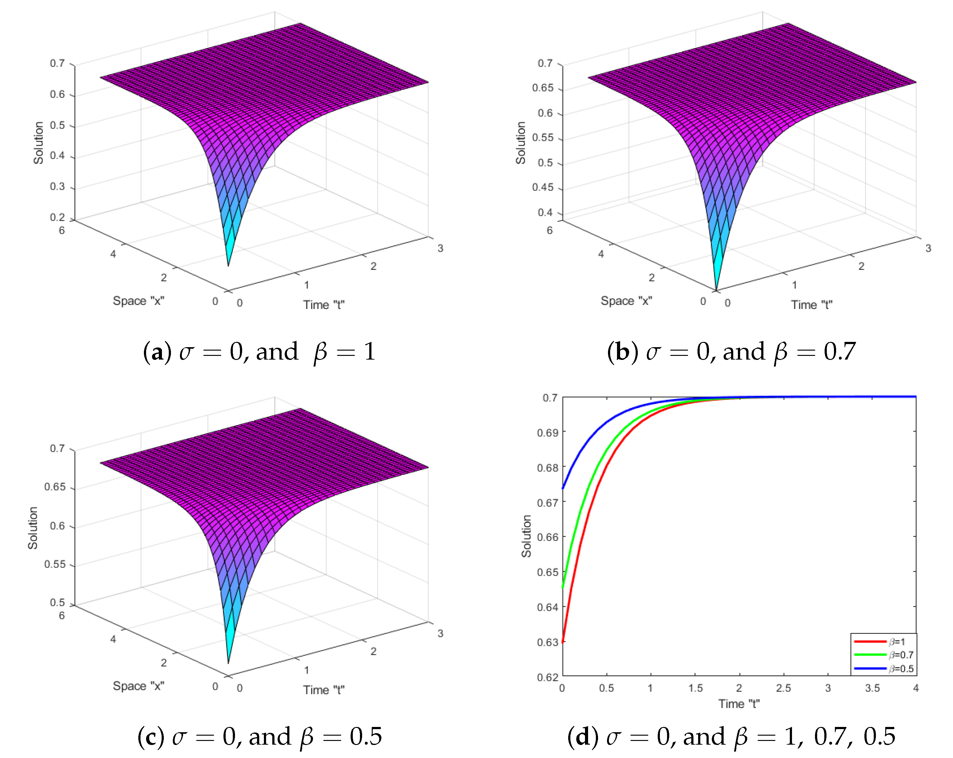
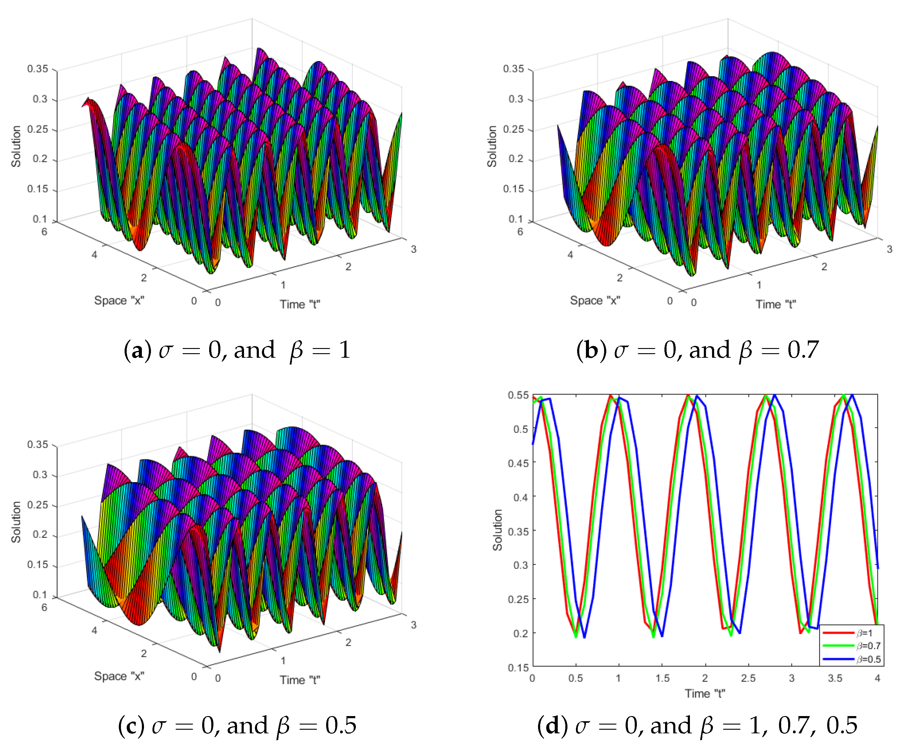
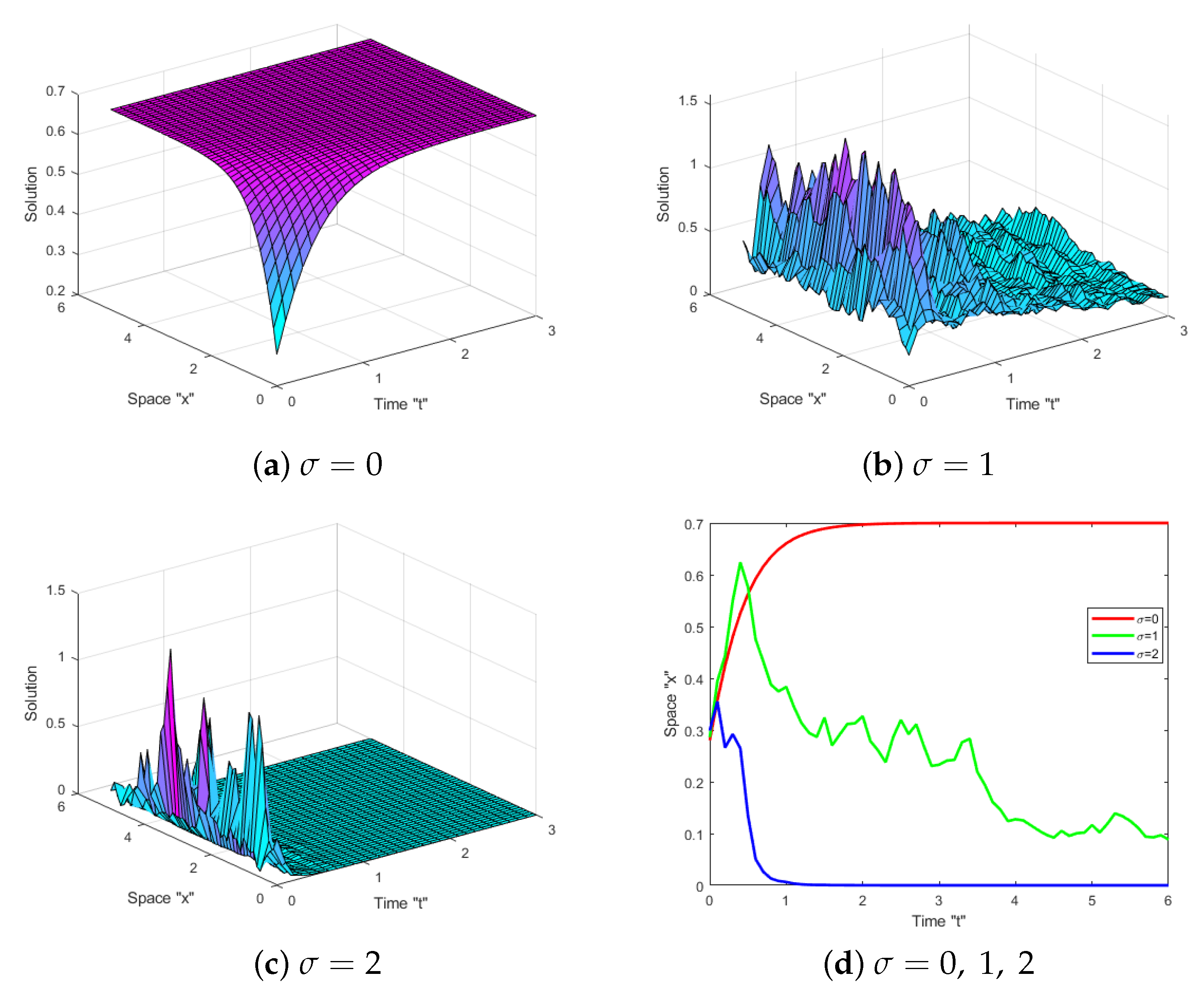
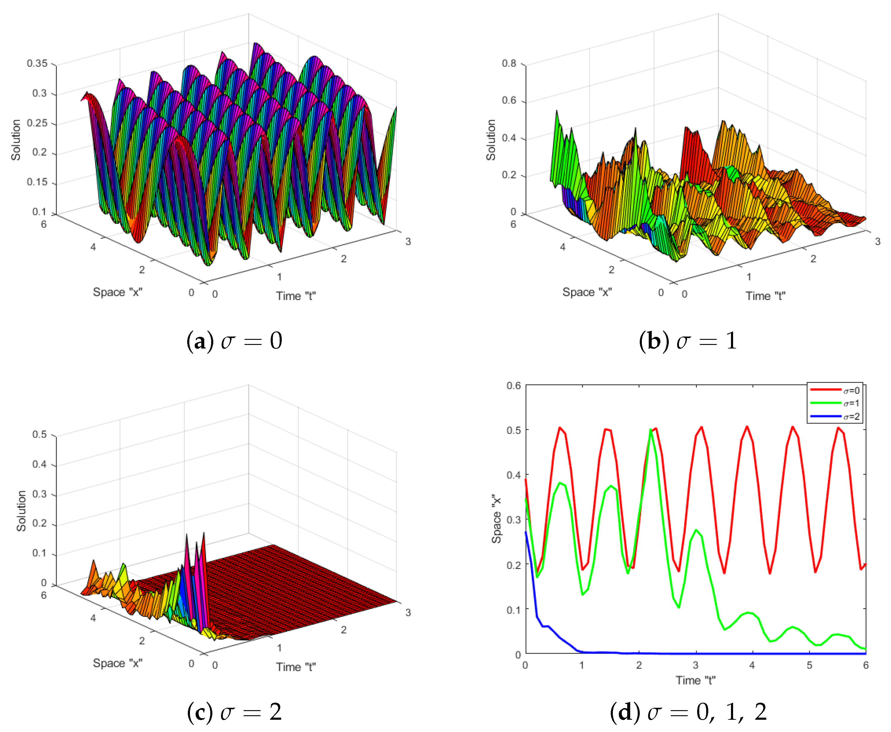
4. Impacts of the Beta Derivative and Noise on SBBME-BD Solutions

We discuss the impact of the BD and white noise on the exact solutions of the SBBME-BD (1). To demonstrate the behavior of these solutions, we provide various graphs. For a different σ (noise intensity), we run some simulations for acquired solutions, including Equations (26) and (32). Let us first fix the parameters ζ 1 = 1 , ϕ = 1 , α = 1 2 and ρ = 0.5 . Moreover, let x [ 0 , 6 ] and t [ 0 , 3 ] .
Effects of the beta derivative: When β decreases, we can observe in Figure 1 and Figure 2 that the form of the graph is compressed:
As we can see in Figure 1 and Figure 2, the solution curves do not intersect. Additionally, the curves shift to the right when the order of the beta derivative increases.
Impacts of white noise: The impact of noise on the solutions is seen in Figure 3 and Figure 4 as follows:
From Figure 3 and Figure 4, we can conclude that there are distinct types of solutions, such as hyperbolic, trigonometric, rational, and Jacobi elliptic solutions, when the noise is ignored (i.e., at σ = 0 ). Adding noise with a strength of σ = 1 , 2 causes the surface to become much flatter following tiny transit patterns, as verified by the 2D graph. This demonstrates that the solutions of SBBME-BD (1) tend to converge around zero when white noise is present.

5. Conclusions

We looked at the stochastic Benjamin–Bona–Mahony Equation (1) with beta derivative (SBBME-BD). The solutions to the Benjamin–Bona–Mahony equation are helpful in understanding several exciting scientific phenomena, such as Rossby waves in rotating fluids and drift waves in plasma. New hyperbolic, trigonometric, rational, and Jacobi elliptic solutions for SBBME-BD were obtained by combining the F -expansion approach with two separate equations, namely the Riccati and elliptic equations. Numerous fascinating and difficult physical occurrences may only be understood with these solutions. The MATLAB program was utilized to investigate the impact of the Gaussian process and beta derivative on the solutions of SBBME-BD (1). It was observed that the white noise component kept the solutions centered around zero. It was concluded that reducing the derivative order resulted in an enlargement of the surface. In future work, we can address Equation (1) with additive noise.

Author Contributions

Data curation, F.M.A.-A. and W.W.M.; formal analysis, W.W.M., F.M.A.-A. and C.C.; funding acquisition, F.M.A.-A.; methodology, C.C.; project administration, W.W.M.; software, W.W.M.; supervision, C.C.; visualization, F.M.A.-A.; writing—original draft, F.M.A.-A.; writing—review and editing, W.W.M. and C.C. All authors have read and agreed to the published version of the manuscript.

Funding

This research received no external funding.

Data Availability Statement

Not applicable.

Acknowledgments

Princess Nourah bint Abdulrahman University Researcher Supporting Project number (PNURSP2023R 273), Princess Nourah bint Abdulrahman University, Riyadh, Saudi Arabia.

Conflicts of Interest

The authors declare no conflict of interest.

References

  1. Zhou, Q.; Ekici, M.; Sonmezoglu, A.; Manafian, J.; Khaleghizadeh, S.; Mirzazadeh, M. Exact solitary wave solutions to the generalized Fisher equation. Optik 2016, 127, 12085–12092. [Google Scholar] [CrossRef]
  2. Alshammari, M.; Iqbal, N.; Mohammed, W.W.; Botmart, T. The solution of fractional-order system of KdV equations with exponential-decay kernel. Results Phys. 2022, 38, 105615. [Google Scholar] [CrossRef]
  3. Zhou, Q.; Zhu, Q. Optical solitons in medium with parabolic law nonlinearity and higher order dispersion. Waves Random Complex Media 2015, 25, 52–59. [Google Scholar] [CrossRef]
  4. Baskonus, H.M.; Bulut, H. New wave behaviors of the system of equations for the ion sound and Langmuir. Waves Waves Random Complex Media 2016, 26, 613–625. [Google Scholar] [CrossRef]
  5. Al-Askar, F.M.; Mohammed, W.W.; Albalahi, A.M.; El-Morshedy, M. The influence of noise on the solutions of fractional stochastic bogoyavlenskii equation. Fractal Fract. 2022, 6, 156. [Google Scholar] [CrossRef]
  6. Manafian, J.; Lakestani, M. Optical solitons with Biswas-Milovic equation for Kerr law nonlinearity. Eur. Phys. J. Plus 2015, 130, 61. [Google Scholar] [CrossRef]
  7. Manafian, J. Optical soliton solutions for Schrodinger type nonlinear evolution equations by the tan(φ/2)-expansion method. Optik 2016, 127, 4222–4245. [Google Scholar] [CrossRef]
  8. Tchier, F.; Yusuf, A.; Aliyu, A.I.; Inc, M. Soliton solutions and conservation laws for lossy nonlinear transmission line equation. Superlattices Microstruct. 2017, 107, 320–336. [Google Scholar] [CrossRef]
  9. Yan, Z.L. Abunbant families of Jacobi elliptic function solutions of the dimensional integrable Davey-Stewartson-type equation via a new method. Chaos Solitons Fractals 2003, 18, 299–309. [Google Scholar] [CrossRef]
  10. Malfliet, W.; Hereman, W. The tanh method. I. Exact solutions of nonlinear evolution and wave equations. Phys. Scr. 1996, 54, 563–568. [Google Scholar] [CrossRef]
  11. Katugampola, U.N. New approach to a generalized fractional integral. Appl. Math. Comput. 2011, 218, 860–865. [Google Scholar] [CrossRef]
  12. Katugampola, U.N. New approach to generalized fractional derivatives. Bull. Math. Anal. Appl. 2014, 6, 1–15. [Google Scholar]
  13. Kilbas, A.A.; Srivastava, H.M.; Trujillo, J.J. Theory and Applications of Fractional Differential Equations; Elsevier: Amsterdam, The Netherlands, 2016. [Google Scholar]
  14. Samko, S.G.; Kilbas, A.A.; Marichev, O.I. Fractional Integrals and Derivatives, Theory and Applications; Gordon and Breach: Yverdon, Switzerland, 1993. [Google Scholar]
  15. Atangana, A.; Baleanu, D.; Alsaedi, A. Analysis of time-fractional Hunter-Saxton equation: A model of neumatic liquid crystal. Open Phys. 2016, 14, 145–149. [Google Scholar] [CrossRef]
  16. Mohammed, W.W. Stochastic amplitude equation for the stochastic generalized Swift–Hohenberg equation. J. Egypt. Math. Soc. 2015, 23, 482–489. [Google Scholar] [CrossRef]
  17. Imkeller, P.; Monahan, A.H. Conceptual stochastic climate models. Stoch. Dynam. 2002, 2, 311–326. [Google Scholar] [CrossRef]
  18. Mohammed, W.W.; Blömker, D. Fast-diffusion limit for reaction-diffusion equations with multiplicative noise. Stoch. Anal. Appl. 2016, 34, 961–978. [Google Scholar] [CrossRef]
  19. Al-Askar, F.M.; Cesarano, C.; Mohammed, W.W. The analytical solutions of stochastic-fractional Drinfel’d-Sokolov-Wilson equations via (G’/G)-expansion method. Symmetry 2022, 14, 2105. [Google Scholar] [CrossRef]
  20. Mohammed, W.W.; Al-Askar, F.M.; Cesarano, C. The analytical solutions of the stochastic mKdV equation via the mapping method. Mathematics 2022, 10, 4212. [Google Scholar] [CrossRef]
  21. Al-Askar, F.M.; Mohammed, W.W. The Analytical Solutions of the Stochastic Fractional RKL Equation via Jacobi Elliptic Function Method. Adv. Math. Phys. 2022, 2022, 1534067. [Google Scholar] [CrossRef]
  22. Mohammed, W.W.; Cesarano, C. The soliton solutions for the (4+1)-dimensional stochastic Fokas equation. Math. Methods Appl. Sci. 2023, 46, 7589–7597. [Google Scholar] [CrossRef]
  23. Alhamud, M.; M Elbrolosy, M.; Elmandouh, A. New Analytical Solutions for Time-Fractional Stochastic (3+ 1)-Dimensional Equations for Fluids with Gas Bubbles and Hydrodynamics. Fractal Fract. 2023, 7, 16. [Google Scholar] [CrossRef]
  24. Elmandouh, A.; Fadhal, E. Bifurcation of Exact Solutions for the Space-Fractional Stochastic Modified Benjamin–Bona–Mahony Equation. Fractal Fract. 2022, 6, 718. [Google Scholar] [CrossRef]
  25. Benjamin, T.B.; Bona, J.L.; Mahony, J.J. Model Equations for Long Waves in Nonlinear Dispersive Systems. Philos. Trans. R. Soc. Lond. Ser. Math. Phys. Sci. 1972, 272, 47–78. [Google Scholar]
  26. Manafianheris, J. Exact solutions of the BBM and MBBM equations by the generalized (G/G)-expansion method equations. Int. J. Genet. Eng. 2012, 2, 28–32. [Google Scholar] [CrossRef]
  27. Das, A.; Ganguly, A. A variation of (G/G)-expansion method: Travelling wave solutions to nonlinear equations. Int. J. Nonlinear Sci. 2014, 17, 268–280. [Google Scholar]
  28. Alsayyed, O.; Jaradat, H.M.; Jaradatd, M.M.; Mustafad, Z.; Shatate, F. Multi-soliton solutions of the BBM equation arisen in shallow water. J. Nonlinear Sci. Appl. 2016, 9, 1807–1814. [Google Scholar] [CrossRef]
  29. Singh, K.; Gupta, R.K.; Kumar, S. Benjamin–Bona–Mahony (BBM) equation with variable coefficients: Similarity reductions and Painlevé analysis. Appl. Math. Comput. 2011, 217, 7021–7027. [Google Scholar] [CrossRef]
  30. Jahania, M.; Manafian, J. Improvement of the exp-function method for solving the BBM equation with time-dependent coefficients. Eur. Phys. J. Plus 2016, 131, 54. [Google Scholar] [CrossRef]
  31. Gündogdu, H.; Gözükizil, O.F. Solving Benjamin-Bona-Mahony equation by using the sn–ns method and the tanh-coth method. Math. Moravica 2017, 21, 95–103. [Google Scholar] [CrossRef]
Figure 1. (ac) show the 3D shapes of Equation (26) with σ = 0 and different values of β = 1 , 0.7 , 0.5 (d) Depicts a graph in two dimensions for these values of β .
Axioms 12 00447 g001
Figure 2. (ac) show the 3D shapes of Equation (32) with σ = 0 and various values of β = 1 , 0.7 , 0.5 (d) Depicts a graph in two dimensions for these values of β .
Axioms 12 00447 g002
Figure 3. (ac) show the 3D shapes of the solution Q ( x , t ) to Equation (26) for various values of σ = 0 , 1 , 2 (d) Depicts a graph in two dimensions for these values of σ .
Axioms 12 00447 g003
Figure 4. (ac) show the 3D shapes of the solution Q ( x , t ) to Equation (32) for various values of σ = 0 , 1 , 2 (d) Depicts a graph in two dimensions for these values of σ .
Axioms 12 00447 g004
Disclaimer/Publisher’s Note: The statements, opinions and data contained in all publications are solely those of the individual author(s) and contributor(s) and not of MDPI and/or the editor(s). MDPI and/or the editor(s) disclaim responsibility for any injury to people or property resulting from any ideas, methods, instructions or products referred to in the content.

