Article

Density-Distance Outlier Detection Algorithm Based on Natural Neighborhood

School of Mathematics and Statistics, Xidian University, Xi’an 710126, China
*
Author to whom correspondence should be addressed.
Axioms 2023, 12(5), 425; https://doi.org/10.3390/axioms12050425
Submission received: 2 March 2023 / Revised: 20 April 2023 / Accepted: 25 April 2023 / Published: 26 April 2023
(This article belongs to the Special Issue Combinatorial Optimization & Applications)

Abstract

:
Outlier detection is of great significance in the domain of data mining. Its task is to find those target points that are not identical to most of the object generation mechanisms. The existing algorithms are mainly divided into density-based algorithms and distance-based algorithms. However, both approaches have some drawbacks. The former struggles to handle low-density modes, while the latter cannot detect local outliers. Moreover, the outlier detection algorithm is very sensitive to parameter settings. This paper proposes a new two-parameter outlier detection (TPOD) algorithm. The method proposed in this paper does not need to manually define the number of neighbors, and the introduction of relative distance can also solve the problem of low density and further accurately detect outliers. This is a combinatorial optimization problem. Firstly, the number of natural neighbors is iteratively calculated, and then the local density of the target object is calculated by adaptive kernel density estimation. Secondly, the relative distance of the target points is computed through natural neighbors. Finally, these two parameters are combined to obtain the outlier factor. This eliminates the influence of parameters that require users to determine the number of outliers themselves, namely, the top-n effect. Two synthetic datasets and 17 real datasets were used to test the effectiveness of this method; a comparison with another five algorithms is also provided. The AUC value and F1 score on multiple datasets are higher than other algorithms, indicating that outliers can be found accurately, which proves that the algorithm is effective.

1. Introduction

With the advance of information science, more data are being collected into databases, storing a large amount of information for science, governments, businesses, and society [1]. Most scientific research focuses on constructing a general pattern map for most data. However, abnormal data are often more valuable than normal data because they often represent a small number of the most specific features. Outlier detection is a significant, emerging, and promising research direction [2]. As a part of data mining, it is the highest priority in many domains; for example, intrusion detection, bank fraud [3], credit analysis, and wireless sensor abnormality detection [4]. It is also a method of preprocessing data in data mining, or can be used as a standalone tool for discovering certain, specific, and implicit pieces of information in a data sample. Its task is to find data whose characteristics are completely different from most of the data features, which are called “outliers”.
In recent decades, outliers were not valued by researchers, but were treated as “by-products” or “noise” of data mining methods. In 1980, Hawkins [5] defined an outlier in his classic book “Identification of Outliers”: outliers behave relatively differently from most data objects in a dataset, so it is suspected that the object is caused by other mechanisms. In recent years, many scholars have been working on finding more efficient and reliable outlier-detection algorithms. In general, three major categories of outliers can be detected [6]: supervised outlier detection, semi-supervised outlier detection and unsupervised outlier detection. In supervised and semi-supervised modes, the model is built from the training dataset and it takes both time and labor to label the dataset. Conversely, unsupervised modes do not need training datasets and can be divided into global and local detection algorithms [7]. Therefore, this paper mainly studies unsupervised outlier detection methods.
In recent years, researchers have proposed various unsupervised outlier detection algorithms, including statistics-based, distance-based [8,9,10], clustering-based [11], and density-based algorithms [3,12]. However, the most common detection methods are based on distance or density.
The study of outliers began with statistical learning models, especially in the field of statistical learning methods. If a data object deviates too much from the standard distribution, it is considered an outlier [13]. Outlier detection methods based on statistical learning are relatively simple to use, and the application of the model does not require much change; however, there are high requirements regarding the users’ knowledge of the dataset. Therefore, this method is not suitable for datasets with unknown conditions.
The distance-based method does not need to assume the distribution of any data. Most methods use existing distance measurement methods to calculate the distance between all data objects, and identify anomaly values according to the distance relationship. The D B ( ε , π ) -outliers approach proposed by Knorr and Ng [14] is a classical distance-based method, and K-nearest neighbor (KNN) distance is used to calculate outlier scores [15]. These methods have relatively intuitive concepts and are easier to understand, but cannot detect outliers in areas of different densities. Meanwhile, it is difficult to determine the threshold of the distance, which is critical for detection performance. Clustering-based methods will find some outliers that do not pertain to any cluster in the process of clustering, and these points called outliers [16,17].
In the density-based method, if the density of the calculated target point is lower than its nearest neighbor’s density, it is called an outlier. The earliest algorithm is the local outlier factor (LOF) [18]. The following research [19] shows that LOF judges outliers according to the score of each point. Next, several extensions of the LOF model appeared, such as the connection-based outlier (COF) [19]. This approach is very similar to LOF; the only difference is the way the density estimate is calculated. The weakness of this approach is that the data distribution is indirectly assumed, which will lead to poor density estimation. The local density factor (LDF) [20] has a certain robustness, which is a further improvement to the LOF algorithm. With regard to kernel density estimation, several new methods have also been introduced recently. An outlier score based on relative density (RDOS) [21] is proposed to measure the local outliers of the target point. Meanwhile, the extended nearest neighbors of the object are considered, and these neighbors are used to further use the local kernel density estimation. The adaptive-kernel density [22] approach is assigned an outlier score to show local differences, and uses an adaptive kernel to improve the recognition ability. In 2018, a relative kernel density [23] not only calculated the local density of the data points, but also calculated the density fluctuations between the fixed point and the adjacent points to further improve the accuracy. Next, Wahid et al. [24] adopted the weighted kernel density estimation (WKDE) method. This not only uses self-adaptation, but also adds weight to the density, and uses extended nearest neighbor to calculate the score of outliers. Local-gravitation outlier detection (LGOD) [25] introduces the concept of inter-sample gravity, which determines the extent of the anomalies by calculating the change in the gravity of a sample’s nearest neighbours. The average divergence difference (ADD) [26] algorithm introduces the concept of average divergence difference to improve the accuracy of local outlier detection. Although the density of clusters in the datasets used varies greatly, the proposed methods have certain effects. However, if there are low-density patterns in the provided data, these methods will not accurately determine the outliers, and the effect will be degraded [19]. Density-based methods tend to be insensitive to global outliers.
In this study, we propose a new method to further calculate local density and relative distance based on natural neighborhood, where natural neighborhoods are neighbors to each other, and there is no need to manually determine neighborhood parameters. Combinatorial optimization is mainly to find optimal object from a limited set of objects. To find outliers through the combination of density and distance, through the fusion of these two measures, this method can be applied to low-density modes without setting the number of neighbors. First, an adaptive kernel density estimation method is proposed to compute the density of the target point. After the density of each target point is determined, the relative distance is introduced. The relative distance is mainly used to judge the proximity between the target object and the object in its own natural neighborhood set, which is mainly composed of the average distance from the target point to its natural neighbors and the distance between natural neighbors. Combining density and distance, a comprehensive outlier factor is obtained to more accurately detect outliers in the dataset. Compared with the current single-parameter outlier detection algorithm, this paper introduces the outlier factor of a two-parameter combination to judge the outlier. The main innovations of the article are summarized as below:
(1)
The natural neighborhood is introduced into outlier detection, and iteration is used to determine the number of neighbors.
(2)
A calculation method of adaptively setting kernel width is proposed to improve the discrimination ability of outlier detection.
(3)
The density and distance are combined to form a new outlier factor.
(4)
We set a suitable threshold as the boundary value to determine whether the object is abnormal, so that the final result does not consider the top-n problem.
The remainder of this article is outlined below. Section 2 presents the preparatory work used to develop the improved method. Section 3 presents the improvement method put forward in this paper. Section 4 contains the comparison and analysis of the experimental results of some outlier detection methods and the improved methods. Finally, Section 5 contains the conclusion and future work directions.

2. Related Work

2.1. Parzen Window for Outlier Detection

Parzen window evaluation, known as the kernel density estimate (KDE), studies the distribution properties from the data samples themselves. There is no need to add any prior knowledge, and there is no additional assumption for the data scatter. Therefore, this is highly valued in the field of statistical theory and application. There are several kernel functions, and the Gaussian kernel is commonly used. The Gaussian kernel is a classical robust radial-basis kernel, which can resist the influence of noise in datasets.
To detect abnormal values in datasets, we can use kernel density estimation to obtain the density of all samples in the set and only compare the density with the threshold to establish the outliers. Although this nonparametric approach does not require any assumptions, it tends to perform poorly for real-world datasets with multiple clusters of significantly different densities, as demonstrated by the example in Figure 1.
In Figure 1, a red point near the dense cluster and away from the scattered cluster is a local outlier. If we use the density estimation method mentioned above, the density of red points in Figure 1 is higher than that of most points in sparse clustering. Thus, if the threshold is set too small, the local outlier cannot be found; however, if the threshold is too large, the points in the scattered cluster will be regarded as outliers and thus have a high error rate. Therefore, it lacks the ability to identify local density in this case.

2.2. Local Outlier Factor

Local outlier factor (LOF) [18] is a density-based outlier detection algorithm that introduces, for the first time, the idea of local outliers that are significant to many algorithms. For every target point, LOF calculates the ratio of its density to the density of adjacent points, yielding its local outlier factor to indicate the extent of the outlier. The parameter k is very important for determining the outlier factor in LOF. The function of parameter k is to obtain the k points that are closest to the target point, also known as k-nearest neighbors, to determine the distance between the k-th nearest neighbor point and the target point, known as the k-distance. Some simple definitions of LOF are as follows:
Definition 1 
([18]). The reachability distance of point p w.r.t. point q is defined as:
r e a c h - d i s t ( p , q ) = max k - distance ( q ) , d i s t ( p , q )
An example of Formula (1) is shown in Figure 2. For different points p 1 and p 2 , their reachable distances are different. For point p 1 , because p 1 is in the k-neighborhood of o ( k = 4 ), its reachable distance is k -distance(o), which is equal to the radius of the circle; and for point p 2 , it is clear that p 2 is not in the k-neighborhood of o, so its reachable distance is their actual distance.
Definition 2 
([18]). The local reachability density (LRD) of point p is the inverse of the average reachability distance of the k near neighbors of point p, which can be defined by:
L R D p = q k n n p r e a c h - d i s t p , q N k p 1
where N k p represents the number of points in the k-th distance of point p.
Definition 3 
([18]). The local outlier factor(LOF) of point p is defined by:
L O F p = q k n n p L R D q L R D p N k p
The outlier factor score for the object p reflects the extent to which we call p outliers. It is determined by the ratio of p to p’s neighbor density. Obviously, if the value of the outlier factor at the p point is greater than 1, p is more likely to be an outlier.

3. Proposed Method

The density-distance outlier detection algorithm based on natural neighborhood does not need to manually define the number of neighbors. If only density is used as the measurement condition, the boundary points will often be mistaken for outliers, and will increase with the increase in parameters. Therefore, we introduce the relative distance to eliminate the interference of boundary points and increase the difference between boundary points and outliers. Through the fusion of density and distance, a comprehensive outlier factor is obtained for evaluation.

3.1. Natural Neighbor

Natural neighbor is an extended concept of a neighbor, which has a stable structure. The understanding of objective reality gave birth to this concept. The number of real friends a person has should be the number of people who mutually regard him or her as their friend. For a data instance, if x thinks that y is a neighbor, and y also acknowledges that x is a neighbor, then object y is one of the natural neighbors of object x. The whole calculation process of natural neighbors can be completed automatically without any parameters. Therefore, the natural neighborhood stability structure formula of the data object is as follows:
x p x q k N x p x q x q K N N k x p x p K N N k x q
where K N N k x p is the k nearest neighbors of object x p .
The k-nearest neighbor of object x p refers to the collection of all points in the dataset whose distance from x p is not greater than that between x p and its k-th neighbor. The formation process of the stable structure of natural neighbors is as follows: the search of neighbor range is expanding, from 1 to λ ( λ as natural neighbor eigenvalue (NaNE)). The NaNE refers to the minimum k value when the algorithm termination condition is satisfied. In each search, the number of reverse neighbors of each instance in the dataset is calculated and the following conditions are judged: (1) all instances have reverse neighbors; (2) the number of instances without reverse neighbors remains unchanged. The reverse neighbor of a target object refers to an object that treats the target object as one of its k-nearest neighbors. When any of the above conditions is satisfied, the stable structure of natural neighbors has been formed. Then our NaNE value is equal to the k value used in the search. λ is obtained by the following formula.
λ = min k | p = 1 n f n b k x p = 0 or p = 1 n f n b k x p = p = 1 n f n b k 1 x p
where n b k x p is the number of reverse nearest neighbors of x p in iteration k. f x is defined as follows:
f x = 1 if x = 0 0 otherwise
Definition 4 
(natural neighbors). The natural neighbor of x p is the neighbor when k iterates to the natural neighbor eigenvalue, which is defined as follows:
N a N x p = K N N λ x p
Algorithm 1 shows the search algorithm process of natural neighbors.
Algorithm 1: Natural Neighbor Search Algorithm
    Axioms 12 00425 i001

3.2. Local Density Estimation

Generally speaking, density is a measure of how close a data object is to its neighborhood objects, and which method to use to estimate the density is also crucial. We adopted adaptive Gaussian kernel density estimation, which greatly reduces the dependence of kernel function on required parameters.
For a present dataset X = x 1 , x 2 , , x n , where X i R d for i = 1 , 2 , , m , the distribution density can be computed as:
ρ ( x ) = 1 n i = 1 n h i d K x x i h i
where K · indicates the kernel function and h i is the width that controls the smoothness of the kernel density function. 1 / n and h d standardize the density estimation and make it integral to 1 in the range of x. Kernel functions satisfy the following expression [27]. The distribution estimate in Formula (8) provides a lot of good features, such as being nonparametric, continuous, and differentiable [28].
K x d x = 1 , x K x d x = 0 , a n d x 2 K x d x > 0
In the classical density problem, estimated previously using the Parzen window, all points use a fixed width parameter h. However, the estimation results of the kernel function are different for the width. Against the background of anomaly detection, the favorable setting of kernel width is the exact opposite of density evaluation. In areas with a high density, we tend not to care about these interesting structures, because they do not provide any value for the determination of outliers. Larger widths may lead to over-smoothing and structure cleaning, but in the low-density region, smaller widths may lead to noise estimation. Therefore, the best choice of width may depend on its specific location in the data space.
Below is a concrete example: consider a 1D dataset 1 , 2 , 3 , 4 , 5 , 10 . The last one is suspected to an exception. Suppose we can correctly apply the above ideas; then, the dataset can be converted to 2.8 , 2.9 , 3 , 3.1 , 3.2 , 20 . Finally, we can more clearly see that the last one is an anomaly.

3.3. Adaptive Kernel Width

At present, we further consider the adaptive setting of the width h i in the Formula (10). Considering the effect of kernel width, we strictly limit this to numbers greater than 0. Considering the ith point, the average distance to its natural neighbor is expressed by d λ x i ; i.e., d λ x i = 1 / λ j N a N ( x i ) d x i , x j . Then, we let d λ max and d λ min show the maximum and minimum quantity in the set d λ x i , respectively. Similar to Silverman’s rule [29], the rough estimation of point density can be expressed by d λ x i , and then the negative correlation among width h i and d λ x i is constructed. Through the above demands, the adaptive width is defined by the following formula:
h i = c d λ max + d λ min + ε d λ x i
where scaling factor c ( c > 0 ) controls smoothing result, ε is a very small number used to ensure that the core width is not 0 (e.g., 10 5 ). This method of setting the core width has two advantages: (a) it improves the discriminative power of the outlier metric; (b) it smoothes the difference between normal samples’ difference. The term d λ max + d λ min was introduced for two reasons. Firstly, the calculated width must be positive. Secondly, even if there is no scale factor c, the denominator width and numerator in the index of Formula (11) will be in the same proportion.
With the adaptive width, the local density of the target point can be expressed as ρ x i . We can see that the measure of local density in our proposed method is not necessarily probability density. Therefore, it is not necessary to normalize the formula. The most common Gaussian kernel is used as the kernel function; then, the local density of ith point is as follows:
ρ x i = 1 n 1 j 1 , 2 , , n \ i exp x i x j h i 2
The right side of Formula (11) does not include the contribution of the target point itself ( exp x i x i 2 / h i 2 = 1 ). The relative difference in density can be reflected (for example, the quantity 0.2 / 0.5 is much smaller than the quantity 1.2 / 1.5 ).

3.4. Relative Distance

In previous density outlier detection methods, outliers can be determined only by kernel density estimation. However, in order to detect outliers more accurately and overcome the problem that local density cannot be used to detect low-density patterns, this paper also considers the influence of the relative distance of the target points.
The relative distance mainly examines the closeness of the object to the object in its own natural neighborhood set, which is composed of natural neighborhood distance and internal neighborhood distance. First, the formula for the natural neighborhood distance is shown in Formula (12).
d ¯ x p = 1 λ x i N a N x p d i s t x i , x p
where d ¯ x p is the natural neighborhood distance of the object x p , x i is an object in the natural neighbor set of object x p , and d i s t x i , x p is the Euclidean distance between object x i and object  x p .
The natural neighborhood distance is actually an average distance, which is the average of the sum of the distances from each object in the candidate set to each object in its own natural neighbor set. Next, the internal neighborhood distance is determined, the formula is as follows:
D ¯ x p = 1 λ λ 1 x i , x j N a N x p , i j d i s t x i , x j
where D ¯ x p is the internal neighborhood distance of the object x p , d i s t x i , x j is the Euclidean distance between object x i and object x j .
The internal neighborhood distance is the average sum of the two distances of all natural neighbor objects using object x p . After calculating the natural neighborhood distance and internal neighborhood distance of all points in the set, the relative distance of the objects can be obtained, as shown in Formula (14).
R D x p = d ¯ x p D ¯ x p

3.5. Density-Distance Outlier Detection Algorithm Based on Natural Neighborhood

It is difficult to raise the accuracy of the algorithm by using a single outlier factor as the key factor for judging outliers. Therefore, the combinatorial optimization problem of combining multiple factors to judge outlier gradually appears. Through the above-mentioned arguments, the algorithm steps are as follows:
(1)
Compute the natural neighborhood of the target object;
(2)
Compute the local density of the target object;
(3)
Compute the relative distance of the target object;
(4)
The calculation formula of the comprehensive outlier factor is obtained.
After evaluating the local density and relative distance of each point, the outlier factor of the object x p can be determined, and a new algorithm, TPOD, is proposed, as defined below:
T P O D ( x p ) = R D x p ρ x p
Density focuses on the degree of correlation between objects, while distance focuses on the degree of deviation between objects. Combining the characteristics of density and distance outlier detection methods, a new algorithm, TPOD, is proposed. The ratio of distance to density is used to determine the calculation of a new outlier factor. Using different outlier factors is important for outlier detection results. Algorithm 2 shows the pseudo-code of this method.

3.6. Threshold

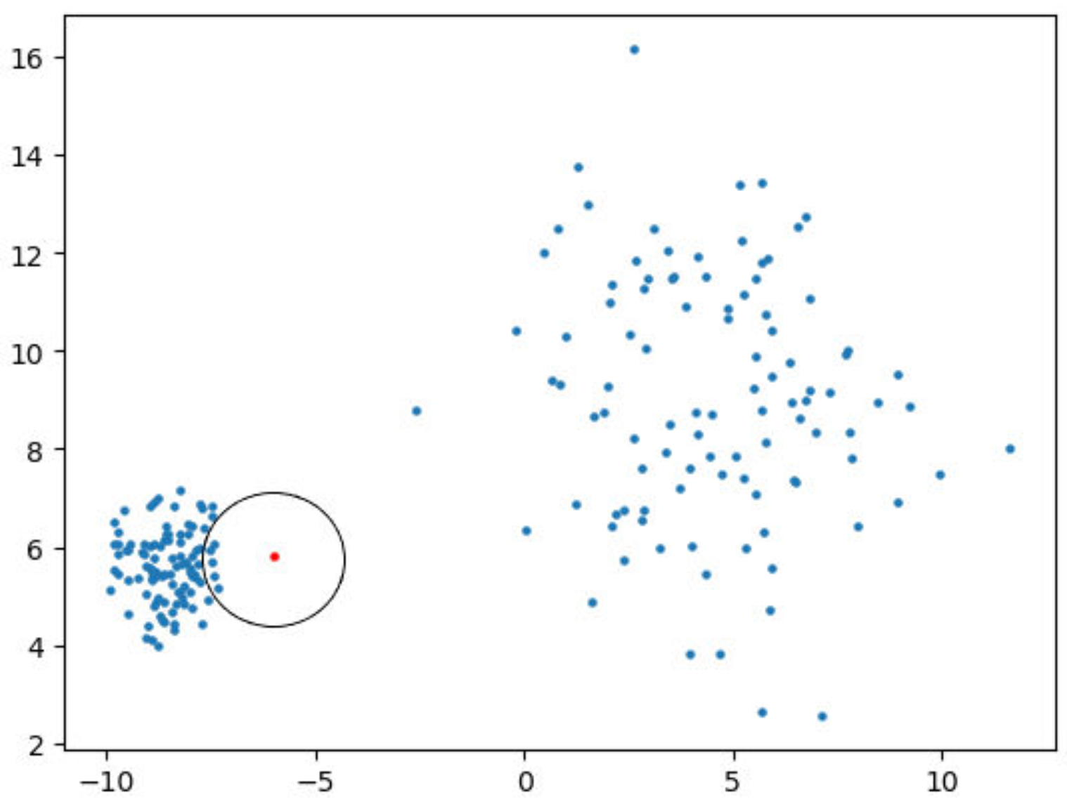
The outlier score of data points in sparse areas is much higher than that in dense areas. In other words, we can set the threshold as the boundary to divide normal points and abnormal points. Therefore, we provide a new method for setting suitable thresholds, as shown below:
σ = η i = 1 n T P O D ( x i ) n
where T P O D ( x i ) refers to the TPOD value of the data point x i , and η is a coefficient, determined by experience. After experimental verification, η is usually 0.2 on synthetic datasets and 0.01 on real datasets. In general, if the TPOD value of the data point is smaller than the preset threshold σ , then the data point is part of the normal range. Conversely, it will be deemed an abnormal value.
Algorithm 2: A Density-Distance Approach for Outlier Detection
    Axioms 12 00425 i002

3.7. Time Complexity Analysis

In this section, we analyzed the time complexity of the algorithm, as follows: In the first stage of the process of searching for natural neighbors, the KD tree was used to search for neighbor information, and its computational time complexity was O n log n , where n refers to the number of datasets. For the formation of a stable structure of natural neighbors, we conducted a λ -step iteration, and the time complexity of this search process was O λ n . The second step is to calculate the local density and relative distance of each point, using its natural neighbor information, so its time complexity is O λ n . Finally, we relied on these two values to obtain the final TPOD score, with a time complexity of O 1 . In summary, we finally obtained that the complexity of our proposed algorithm is O n log n .

4. Experimental and Results Analysis

4.1. Experimental Dataset

The dataset used in the experiment was divided into two parts: an artificial synthetic dataset and real dataset, and the effectiveness of the algorithm was verified from two directions.
(1)
Artificial synthetic datasets
The first dataset contained three clusters, and the cluster centers were (−7, −7), (−3, 9), and (5, 2). There was a total of 239 sample points, of which 14 were outliers. The points in the second dataset were distributed near the cosine curve. There was a total of 194 sample points, of which 5 were outliers. In Figure 3, we show the distribution of points in these synthetic datasets.
(2)
Real-life datasets
In the outlier detection algorithm, the preprocessing operation of the dataset is very important. The selection of a suitable dataset occured pre-operation, and the preprocessing of the dataset occured post-operation. Our outlier detection experiments were also evaluated on real datasets to assess the effect of various outlier detection algorithms. These datasets were all from the datasets or variants of the UCI standard [30], and have been applied by many previous studies. The datasets used in this paper were the same version as the datasets used in the literature. A description of the dataset is shown in Table 1. In [31], we obtained two types of dataset: the previously frequently used outlier detection datasets and some semantic outlier datasets. At the same time, preprocessing was carried out before reusing these datasets. The specific processing process is as follows:
a.
1-of-n encoding: This can convert non-numeric data in the dataset into numeric data. A categorical attribute with n possible values in a 1-of-n encoding maps to n binary attributes, where 1 indicates that the value of the relevant attribute exists, while 0 indicates that it does not exist.
b.
Normalization: The values of all numerical attributes are all normalized to the range of [ 0 , 1 ] .
In Table 1, we present basic information of the 17 datasets used, which are commonly used to evaluate classification methods. In the field of anomaly detection, a few categories in the classified data are regarded as outliers. We also analyzed the background knowledge of some datasets to explain the difference between the distribution of normal data and outlier data in the datasets. The 17 datasets we used contain 148–9868 data, and the dimensions ranged from 7 to 57. In the HeartDisease dataset data on heart health are collected, in which infected people are called outliers, while healthy people are normal. In addition, the spambase dataset and the mail collection show that 1813 spam messages are abnormal, and the rest are normal.

4.2. Experimental Setup

The experiments in this section were carried out on a computer with the Intel core i7-6700 processor platform, 3.40-GHz frequency, 8-GB memory. The operating system is Windows 10. The experiments were performed in Python 3.8.
There are many indicators to assess the performance of outlier detection, for instance accuracy, precision, and F 1 score [32]. However, since many datasets related to anomaly detection are unbalanced, some indicators are not suitable for application in this paper. The main evaluation indicators we adopted were AUC and F 1 score [12]. F 1 score is a comprehensive evaluation index combining precision and recall. Its calculation formula is shown in Formula (17). False positive rate ( F P R ) and true positive rate ( T P R ) are used in the ROC curve. The formula is shown in Formulas (18) and (19).
F 1 = 2 p r e c i s i o n r e c a l l p r e c i s i o n + r e c a l l
F P R = F P F P + T N
T P R = T P T P + F N
The descriptions of these indicators are shown in Table 2. The accuracy rate refers to how many of the samples that we predicted were correct, and the recall rate refers to how many of the samples that were actually correct were selected by us. When evaluating a model, we hope that the accuracy rate and recall rate are both high, but we cannot have both. Therefore, the F 1 score considers the factors of precision and recall, and reconciles the two, which can evaluate the quality of the model. The greater the F 1 score, the better the effect of the model.

4.3. Experimental Results Analysis

Firstly, we tested the performance of the TPOD method on the two synthetic datasets. The first composite dataset consists of three clusters centered on (−7, −7), (−3, 9) and (5, 2), respectively. In our new method, TPOD, we made use of c = 0.9 in kernel functions. The calculated TPOD scores were ranked, and the first 14 of the Gaussian dataset are listed in Table 3.
The top five TPOD values of the cosine dataset are shown in Table 4. This shows that the effectiveness of our algorithm can accurately distinguish outliers in the dataset.
From the Table 3, we can see that the top 14 pieces of data are all the data points shown in Figure 4a, where the blue points represent inlines, and the red points indicates the abnormal values that were found. From the Table 4, we can see that the top five pieces of data are all the data points shown in Figure 4b, where the cyan points represent inlines, and the red points indicate the abnormal values that were found.
Then, in the real dataset, the comparison algorithms used in the experiment were as follows: LOF [18], COF [19], local distance outlier detection(LDOF) [33], angle based outlier detection(ABOD) [34], and a relative density-based outlier score(RDOS) [21]. The five algorithms in the experiment performed outlier detection on 17 datasets. A large number of experiments showed that the value of the parameter c can be selected from the range [ 0.5 , 1 ] . The selection of the k parameter in the comparison method can be performed using the nearest neighbor search method in the literature [35].
For algorithm comparison, we ran six outlier detection algorithms on the dataset in Table 1. After using these methods to calculate outliers, we present the best effects of these methods in Figure 5 and Figure 6. Lines with different colors represent different outlier detection methods. The specific AUC result values are shown in Table 5, and the best results are shown in bold. For example, on the cardiotocography dataset, the optimal AUC value of other comparison methods was 0.5932, and our method TPOD obtained the optimal AUC value of 0.6700. The AUC of the algorithm is 12.9% higher than that of the last ranked algorithm. Meanwhile, for the lymphography dataset, the AUC result obtained by our proposed method can reach 0.9988. Each method achieved low AUC scores on the WPBC dataset. The reason for this is that the class distributions are not very different, so it is difficult to distinguish outliers when using the nearest neighbor concept. Our proposed TPOD method is still the best, indicating that our method can also obtain good results for low-density patterns.
In general, from the above results, we can see that our proposed approach of TPOD has a better performance than the widely used outlier detection algorithm. Of the datasets in Table 1, TPOD showed the best performance. For PenDigits dataset, the AUC score obtained by the TPOD experiment with our method is 0.9792, where the parameter λ = 70 and c = 0.5 . In particular, the TPOD approach achieved the best results for 14 datasets, including Lymphography, WDBC, WPBC, GLASS, Ionosphere, Waveform, Cardiotocography, PageBlocks, Stamps, PenDigits, letter, concrete, Pima, and breastcancer. In the remaining three datasets, HeartDisease, SpamBase and breastcancer, the performance of TPOD was lower than the ABOD, RDOS, and LOF outlier detection methods, respectively. However, in the HeartDisease dataset, the optimal AUC result of TPOD at λ = 12 , c = 0.9 is 0.6261, which is slightly behind the optimal result of the ABOD method at k = 5 ; in the SpamBase dataset, TPOD is at λ = 33 , with the optimal AUC result obtained when c = 0.6 is 0.5216, which is slightly behind the optimal result of the LOF method when k = 68 . Compared to other algorithms, our algorithm considers more comprehensive factors and can more comprehensively reflect the data information. After introducing density, relative distance is further introduced to more accurately detect outliers. For parameters, natural neighbors provide a stable neighborhood structure.
To further affirm the performance of our proposed algorithm, we also calculated the F1 scores on these datasets. As shown in Table 6, the results in bold are the best, and the second best results are expressed by *. For example, in the lymphography dataset, the optimal F1 score result of TPOD at λ = 12 , c = 1 is 0.85, which is greater than the maximum value of 0.83 in our compared methods. Among the 16 datasets in our experiments, our algorithm TPOD performed the best in 9 datasets and the second best in 4 datasets. In general, our algorithm performs well in most datasets.

5. Conclusions

In our daily life, we should not underestimate abnormal situations. For example, the discovery of a rare disease would be a major breakthrough. Focusing on the problem that distance-based outlier detection methods cannot detect local outliers and density-based outlier detection methods cannot handle low-density patterns, we introduce two parameters to combinatorial optimization to overcome these shortcomings. Firstly, the natural neighborhood of the target point was found through iteration, and then adaptive kernel density estimation was used to calculate the local density of the point. Secondly, we computed the relative distance of the target point. Finally, by fusing the density and distance values of the target points to calculate the comprehensive outlier, the outliers could be identified more accurately. We also provided a threshold to determine the final outlier, eliminating the impact of top-n. The experimental results on 2 artificial datasets and 17 UCI real-life datasets show that the effect of this method is the best compared with 5 typical outlier detection methods.
In future work, we plan to extend the outlier detection problem to high-dimensional space. For datasets with a small proportion of outliers, we can further reduce the size of the dataset and remove some outliers that are unlikely to be outliers. In addition, outlier detection methods can be applied in practical applications.

Author Contributions

Conceptualization, J.Z. and Y.Y.; methodology, J.Z.; software, J.Z.; validation, J.Z.; formal analysis, J.Z.; investigation, J.Z.; resources, J.Z.; data curation, J.Z.; writing—original draft preparation, J.Z.; writing—review and editing, J.Z. and Y.Y.; visualization, J.Z.; supervision, Y.Y.; project administration, J.Z.; funding acquisition, Y.Y. All authors have read and agreed to the published version of the manuscript.

Funding

This work was funded by National Natural Science Foundation of China (61573266), Natural Science Basic Research Program of Shaanxi (Program No. 2021JM-133).

Data Availability Statement

https://archive.ics.uci.edu/ml/index.php (accessed on 1 March 2023).

Conflicts of Interest

This authors declare no conflict of interest regarding the publication for this paper.

References

  1. Han, J.; Kamber, M.; Pei, J. Data Mining: Concepts and Techniques Third Edition. Morgan Kaufmann Ser. Data Manag. Syst. 2011, 5, 83–124. [Google Scholar]
  2. Wang, H.; Bah, M.J.; Hammad, M. Progress in outlier detection techniques: A survey. IEEE Access 2019, 7, 107964–108000. [Google Scholar] [CrossRef]
  3. Domingues, R.; Filippone, M.; Michiardi, P.; Zouaoui, J. A comparative evaluation of outlier detection algorithms: Experiments and analyses. Pattern Recognit. 2018, 74, 406–421. [Google Scholar] [CrossRef]
  4. Safaei, M.; Asadi, S.; Driss, M.; Boulila, W.; Safaei, M. A systematic literature review on outlier detection in wireless sensor networks. Symmetry 2020, 12, 328. [Google Scholar] [CrossRef] [Green Version]
  5. Hawkins, D.M. Identification of Outliers; Springer: Berlin/Heidelberg, Germany, 1980. [Google Scholar]
  6. Boukerche, A.; Zheng, L.; Alfandi, O. Outlier detection: Methods, models, and classification. ACM Comput. Surv. 2020, 53, 1–37. [Google Scholar] [CrossRef]
  7. Yang, J.; Rahardja, S.; Fränti, P. Mean-shift outlier detection and filtering. Pattern Recognit. 2021, 115, 107874. [Google Scholar] [CrossRef]
  8. Angiulli, F.; Basta, S.; Lodi, S.; Sartori, C. GPU Strategies for Distance-Based Outlier Detection. IEEE Trans. Parallel Distrib. Syst. 2016, 27, 3256–3268. [Google Scholar] [CrossRef]
  9. Fan, H.; Zaane, O.R.; Foss, A.; Wu, J. Resolution-based outlier factor: Detecting the top-n most outlying data points in engineering data. Knowl. Inf. Syst. 2009, 19, 31–51. [Google Scholar] [CrossRef]
  10. Kontaki, M.; Gounaris, A.; Papadopoulos, A.N.; Tsichlas, K.; Manolopoulos, Y. Efficient and flexible algorithms for monitoring distance-based outliers over data streams. Inf. Syst. 2016, 55, 37–53. [Google Scholar] [CrossRef]
  11. Huang, J.; Zhu, Q.; Yang, L.; Cheng, D.D.; Wu, Q. A novel outlier cluster detection algorithm without top-n parameter. Knowl.-Based Syst. 2017, 121, 32–40. [Google Scholar] [CrossRef]
  12. Hautamäki, V.; Kärkkäinen, I.; Fränti, P. Outlier detection using k-nearest neighbour graph. In Proceedings of the 17th International Conference on Pattern Recognition, Cambridge, UK, 26 August 2004; pp. 430–433. [Google Scholar]
  13. Barnett, V.; Lewis, T. Outliers in Statistical Data; Wiley: New York, NY, USA, 1994. [Google Scholar]
  14. Knorr, E.M.; Ng, R. Algorithms for mining distancebased outliers in large datasets. In Proceedings of the International Conference on Very Large Data Bases, New York, NY, USA, 24–27 August 1998; pp. 392–403. [Google Scholar]
  15. Zhang, Y.; Cao, G.; Wang, B.; Li, X. A novel ensemble method for k-nearest neighbor. Pattern Recognit. 2019, 85, 13–25. [Google Scholar] [CrossRef]
  16. Moshtaghi, M.; Bezdek, J.C.; Havens, T.C.; Leckie, C.; Palaniswami, M. Streaming analysis in wireless sensor networks. Wirel. Commun. Mob. Comput. 2014, 14, 905–921. [Google Scholar] [CrossRef]
  17. Rizk, H.; Elgokhy, S.; Sarhan, A. A hybrid outlier detection algorithm based on partitioning clustering and density measures. In Proceedings of the 2015 Tenth International Conference on Computer Engineering & Systems, Cairo, Egypt, 23–24 December 2015; pp. 175–181. [Google Scholar]
  18. Breunig, M.M.; Kriegel, H.P.; Ng, R.T.; Sander, J. LOF: Identifying density-based local outliers. In Proceedings of the 2000 ACM SIGMOD International Conference on Management of Data, Dallas, TX, USA, 16–18 May 2000; pp. 93–104. [Google Scholar]
  19. Tang, J.; Chen, Z.; Fu, A.; Cheung, D. Enhancing effectiveness of outlier detections for low density patterns. In Proceedings of the Pacific-Asia Conference on Knowledge Discovery and Data Mining, Taipei, Taiwan, 6–8 May 2002; pp. 535–548. [Google Scholar]
  20. Latecki, L.J.; Lazarevic, A.M.; Pokrajac, D.M. Outlier detection with kernel density functions. In Proceedings of the Machine Learning and Data Mining in Pattern Recognition, Leipzig, Germany, 18–20 July 2007; pp. 61–75. [Google Scholar]
  21. Tang, B.; He, H. A Local Density-Based Approach for Outlier Detection. Neurocomputing 2017, 241, 171–180. [Google Scholar] [CrossRef] [Green Version]
  22. Zhang, L.; Jing, L.; Karim, R. Adaptive kernel density-based anomaly detection for nonlinear systems. Knowl.-Based Syst. 2018, 139, 50–63. [Google Scholar] [CrossRef] [Green Version]
  23. Wahid, A.; Sekhar, C.; Deb, K. A relative kernel-density based outlier detection algorithm. In Proceedings of the 12th International Conference on Software, Knowledge, Information Management and Applications, Phnom Penh, Cambodia, 3–5 December 2018; pp. 1–7. [Google Scholar]
  24. Wahid, A.; Sekhar, C. Rkdos: A relative kernel density-based outlier score. IETE Tech. Rev. 2020, 37, 441–452. [Google Scholar] [CrossRef]
  25. Xie, J.; Xiong, Z.; Dai, Q.; Wang, X.; Zhang, Y. A local-gravitation-based method for the detection of outliers and boundary points. Knowl.-Based Syst. 2020, 192, 105331. [Google Scholar] [CrossRef]
  26. Xiong, Z.Y.; Gao, Q.Q.; Gao, Q.; Zhang, Y.F.; Li, L.T.; Zhang, M. ADD: A new average divergence difference-based outlier detection method with skewed distribution of data objects. Appl. Intell. 2022, 52, 5100–5124. [Google Scholar] [CrossRef]
  27. Murphy, K.P. Machine Learning: A Probabilistic Perspective; MIT Press: Cambridge, MA, USA, 2012. [Google Scholar]
  28. Tang, B.; He, H. KernelADASYN: Kernel based adaptive synthetic data generation for imbalanced learning. In Proceedings of the Evolutionary Computation, Sendai, Japan, 25–28 May 2015; pp. 664–671. [Google Scholar]
  29. Zhu, M.; Su, W.; Chipman, H.A. LAGO: A computationally efficient approach for statistical detection. Technometrics 2006, 48, 193–205. [Google Scholar] [CrossRef] [Green Version]
  30. Bache, K.; Lichman, M. UCI machine learning repository. Sch. Inf. Comput. Sci. 2013. [Google Scholar]
  31. Campos, G.O.; Zimek, A.; Schubert, E. On the evaluation of unsupervised outlier detection: Measures, datasets, and an empirical study. Data Min. Knowl. Discov. 2016, 30, 891–927. [Google Scholar] [CrossRef]
  32. Thennadil, S.N.; Dewar, M.; Herdsman, C.; Nordon, A.; Becker, E. Automated weighted outlier detection technique for multivariate data. Control. Eng. Pract. 2018, 70, 40–49. [Google Scholar] [CrossRef] [Green Version]
  33. Zhang, K.; Hutter, M.; Jin, H. A new local distance-based outlier detection approach for scattered real-world data. In Proceedings of the Pacific-Asia Conference on Knowledge Discovery and Data Mining, Bangkok, Thailand, 27–30 April 2009; pp. 813–822. [Google Scholar]
  34. Kriegel, H.P.; Schubert, M.; Zimek, A. Angle-based outlier detection in high-dimensional data. In Proceedings of the 14th ACM SIGKDD International Conference on Knowledge Discovery and Data Mining, Las Vegas, NV, USA, 24–27 August 2008; pp. 444–452. [Google Scholar]
  35. Ning, J.; Chen, L.; Zhou, C.; Wen, Y. Parameter k search strategy in outlier detection. Pattern Recognit. Lett. 2018, 112, 56–62. [Google Scholar] [CrossRef]
Figure 1. Global measurement cannot detect red local outliers.
Axioms 12 00425 g001
Figure 2. Example of reachable distance.
Axioms 12 00425 g002
Figure 3. Artificial dataset distribution. (a) Gaussian synthetic datasets. (b) Cosine synthetic datasets.
Axioms 12 00425 g003
Figure 4. Distribution of outliers identified. (a) Gaussian synthetic datasets. (b) Cosine synthetic datasets.
Axioms 12 00425 g004
Figure 5. AUC values of six methods on nine datasets. (a) Lymphography. (b) WDBC. (c) WPBC. (d) glass. (e) Ionosphere. (f) Waveform. (g) Cardiotocography. (h) HeartDisease. (i) PageBlocks.
Axioms 12 00425 g005
Figure 6. AUC values of six methods on eight datasets. (a) Stamps. (b) Pima. (c) SpamBase. (d) breastcancer. (e) letter. (f) concrete. (g) satellite. (h) PenDigits.
Axioms 12 00425 g006
Table 1. Summarizes the details of each dataset.
Datasetof Featuresof Outliersof Data
Lymphography176148
WDBC3010367
WPBC3347198
GLASS79214
Ionosphere32126351
Waveform211003443
PenDigits16209868
Cardiotocography214712126
HeartDisease13120270
PageBlocks105605473
Pima8268768
SpamBase5718134601
Stamps931340
breastcancer3010357
letter321001600
satellite36755100
concrete85151030
Table 2. Indicator description (P: Positive, N: Negative).
PredictionActualFinal
PPTP
PNFP
NPFN
NNTN
Table 3. The 14 largest TPOD data samples in the Gaussian composite dataset.
DataTPODRank
(−8.5, 10)9.021
(6, −7.5)4.312
(2, 10)3.513
(−6, 2.5)3.114
(0, −6)3.015
(−3.8, 5)2.776
(4, −5)2.497
(3, 8)2.378
(1, 5.2)1.649
(−4, 0)1.6010
(2, −5)1.4711
(−2, 1.9)1.3112
(−3, −8)1.1013
(−2, 0)1.0914
Table 4. The five largest TPOD data samples in the Cosine composite dataset.
DataTPODRank
(0, −1)6.241
(2, 1)5.082
(6, −0.5)4.923
(3, 0)3.264
(8, −1)1.175
Table 5. AUC score of 6 outlier detection methods over 17 datasets.
DatasetsLOFCOFABODLDOFRDOSTPOD
Lymphography0.97300.97070.99650.94250.9965 0.9988
WDBC0.90200.87790.89890.83890.8824 0.9255
WPBC0.51710.46910.51610.69380.8038 0.8688
Ionosphere0.90310.91080.92710.89610.8503 0.9320
Waveform0.76090.74930.70350.69570.7534 0.7849
Cardiotocography0.59320.56790.50970.56340.5933 0.6700
HeartDisease0.54940.5298 0.6391 0.56910.53330.6261
PageBlocks0.81800.76420.70200.82080.6108 0.9113
Stamps0.68830.59530.78680.66260.7254 0.8450
Pima0.61920.60440.70530.56930.6246 0.7271
SpamBase0.47400.49930.41090.4797 0.5337 0.5216
breastcancer 0.9807 0.96270.95320.96470.9437 0.9807
letter0.90730.88210.90630.86580.9229 0.9238
concrete0.65990.67580.68480.59060.6713 0.6960
satellite 0.9701 0.95160.96630.88360.96630.9656
PenDigits0.91670.94720.97110.71330.9719 0.9792
Table 6. F1 score of 6 outlier detection methods over 16 datasets. Note: The second best result is represented by *.
DatasetsLOFCOFABODLDOFRDOSTPOD
Lymphography0.720.660.83 *0.300.49 0.85
WDBC 0.58 0.330.350.310.100.57 *
WPBC0.180.210.280.250.36 * 0.38
GLASS0.30 * 0.33 0.200.170.240.20
Ionosphere0.810.83 0.88 0.710.700.84 *
Waveform0.20 0.26 0.070.120.080.23 *
Cardiotocography0.320.290.330.290.35 * 0.38
HeartDisease0.490.460.54 *0.430.52 0.63
PageBlocks 0.51 0.47 *0.370.450.380.45
Pima0.450.450.500.51 * 0.53 0.53
SpamBase0.310.320.360.430.45 * 0.56
Stamps0.200.190.220.220.27 * 0.35
breastcancer 0.77 0.57 *0.400.210.110.20
letter 0.54 0.500.450.380.220.51 *
satellite0.60 *0.270.460.150.10 0.62
concrete0.610.630.67 *0.67 *0.65 0.69
Disclaimer/Publisher’s Note: The statements, opinions and data contained in all publications are solely those of the individual author(s) and contributor(s) and not of MDPI and/or the editor(s). MDPI and/or the editor(s) disclaim responsibility for any injury to people or property resulting from any ideas, methods, instructions or products referred to in the content.

