1. Introduction
Warrantors and warrantees are the two main types of bodies responsible for managing the through-life reliabilities of products. In the case of dividing a through-life cycle into early and late stages, i.e., its warranty and post-warranty periods, the former main body uses warranty models to manage product reliability during the early stage of the through-life cycle, and the latter main body manages the product reliability during the late stage of the through-life cycle by means of self-maintenance actions.
To efficaciously manage a product’s reliability during the early stage of its through-life cycle, some practitioners have constructed plentiful warranty models on different categories of maintenance models. In the case of classifying exiting maintenance models, warranty models can be divided into three categories. The first category of models could be called traditional warranty models because their basic forms are traditional maintenance models in which the time to the first failure is modeled as a lifetime-distribution function. For example, Chen et al. [
1], Wang et al. [
2], Wang and Ye. [
3], Wang et al. [
4] and Ye et al. [
5] have integrated traditional minimal repair actions into the warranty period or coverage area and constructed repair free warranty (FRW) models. Peng et al. [
6], Wang et al. [
7] and Ruan et al. [
8] have constructed preventive maintenance warranty (PMW) models by integrating traditional preventive maintenance actions into the warranty period or coverage area.; Liu et al. [
9], Qiao et al. [
10] and Wang et al. [
11] have constructed renewing replacement warranty (RRW) models by incorporating traditional replacement actions into the warranty period or coverage area.
The second category of models is called condition-based warranty models because they are based on condition-based maintenance models in Wang et al. [
12,
13], Zhu et al. [
14], Qiu et al. [
15,
16], Zhao et al. [
17], Zhang et al. [
18], Chen et al. [
19] and Yang et al. [
20] wherein the product degradation is measured as any stochastic degradation process according to Zhao et al. [
21,
22], Ye and Xie [
23], Yang et al. [
24]; Qiu et al. [
25,
26,
27,
28,
29] and Zhang et al. [
30]. For example, Zhang et al. [
31] have constructed a renewing free replacement model of a two-component series system by means of a condition-based maintenance model, and Shang et al. [
32] have constructed a condition-based RRW model by integrating condition-based maintenance into the warranty period. The last category of models consists of random warranty models built on the basis of random maintenance models wherein monitored task/working/project/mission cycles are modeled as random variables with an identical distribution function. For example, in the case of assuming working cycles as random variables with an identical distribution function, Shang et al. [
33] modeled a two-dimensional free repair warranty first and a two-dimensional free repair warranty last. As far as we know, in existing warranty models, there rarely exist warranty models that are designed by screening the differences in product reliabilities to control the warranty costs of the products with the different reliabilities.
Considering the management of product reliabilities during the late stage of the through-life cycle as a key factor, warrantees’ self-maintenance models have been widely researched by some practitioners, which are similarly concentrated upon the following three types. ① By means of preventive maintenance actions, Park et al. [
34] and Park and Pham [
35] have researched preventive maintenance models for managing product reliabilities during the late stage of the through-life cycle, which will be hereafter called product reliabilities after the warranty expiration; ② building on the basis of condition-based maintenance, Shang et al. [
32] have presented a condition-based maintenance model to manage product reliabilities after the warranty expiration; and ③ by modeling working cycles as random variables, Shang et al. [
36,
37,
38,
39] have constructed random maintenance models to manage product reliabilities after the warranty expiration. Although Shang et al. [
36] have provided random maintenance models to manage product reliabilities after the warranty expiration, their focuses are limited to the differences in the reliabilities at all expiries of warranty limits, which have been characterized as the different reliability functions of the same product. From the perspective of reliability theory, the differences in the reliabilities of new identical products, e.g., the length of the arrival time to the first failure, have a more significant effect on modeling maintenance policies and controlling maintenance costs. However, as far as we know, in existing maintenance models to manage product reliabilities after their warranty expirations, it is rare to customize the random maintenance model based on the differences in the reliabilities of new identical products in order to control maintenance costs and lengthen service life.
Summing up the above, focusing on products with task cycles, this paper introduces a pre-specified time threshold to the early stage of the through-life cycle for screening the differences in the reliabilities of new identical products. Based on whether the arrival time to the first failure is larger than the pre-specified time threshold, a random warranty model and a random maintenance model are devised to manage the through-life reliabilities of new identical products that survive the burn-in test. Two services with different coverage areas are conditionally used to continue to manage product reliabilities. One service with a larger coverage area is used to manage the reliability of a product in which no failure occurs until the pre-specified time threshold, and another service with a smaller coverage area is used to manage the reliability of a product in which first failure occurs before the pre-specified time threshold. All failures in each coverage area are removed with minimal repair, and the different occurrence cases of the arrival time to the first failure triggers the service with the different coverage areas, and thus this warranty model is a flexible warranty model known as a flexible random free repair warranty (FRFRW) model. Similar to the design of the FRFRW model, the random maintenance model for managing product reliabilities after warranty expiration is customized by a different relationship between the length of the arrival time to the first failure and the pre-specified time threshold. Two random replacements with smaller and larger replacement ranges, respectively, are designed for controlling maintenance costs after the FRFRW expiration. In view of these, such a type of replacement model is called a customized random replacement (CRR) model. Each of the above two random models is characterized from the mathematical perspective, and some related derivatives are provided to model other maintenance problems.
The key novelties of this study are listed as follows: by comparing the arrival time to the first failure and the pre-specified time threshold, a flexible warranty model is designed to warrant new identical products with different reliabilities, which have rarely occurred in the published works. In the case of different relationships between the length of the arrival time to the first failure and the pre-specified time threshold, a random replacement model is customized to manage product reliabilities after the warranty expiration, which is different from published works in which the differences in product reliabilities have been differed by means of reliability functions at all expiries of warranty limits.
The structure of this study is as follows. In
Section 2, the FRFRW is designed by comparing the arrival time to the first failure and the pre-specified time threshold, and the related measures are evaluated from the mathematical perspective. In
Section 3, the CRR model is customized by differing the relationships between the length of the arrival time to the first failure and the pre-specified time threshold, and some of the derivative models are provided to mathematically measure other maintenance problems. In
Section 4, a numerical analysis is performed to dissect unexplored characteristics. In
Section 5, conclusions are presented.
2. Random Warranty Design
The assumptions of this study are listed as follows: all identical products surviving the burn-in test implement tasks at cycles called task cycles, and the task cycles of the () task are independent and identically distributed random variables with a memoryless distribution function given by ; the distribution function of the time to first failure is given by with the failure rate function , wherein () and () are two parameters; and the time to repair/replacement is negligible.
2.1. Random Warranty Definition
Let and be two natural numbers and , and be a time threshold and two extended time spans where . Using such notations, the definition of random warranty is depicted below:
- ◆
If no failure occurs until the time threshold , then such a product will continue to undergo minimal repair at all failures until the extended time span ;
- ◆
If the first failure occurs before the time threshold , then such a failure is removed with minimal repair and the related product will continue to undergo minimal repair at all failures until the task cycle completes or at the extended time span , whichever occurs first.
Notably, no failure occurring until the time threshold
signals that the reliability of the related product is higher than the reliability of the product under the first failure occurring before the time threshold
. These indicate that comparing the relationship between the arrival time to the first failure and the time threshold
is one of the key methods used to screen differences in the reliabilities of new identical products. Furthermore, on the basis of screening results, controlling future warranty costs is more practical for warrantors. From the viewpoint of the measure of coverage area, in the case of
, the coverage area consisting of the extended time span
is greater than the coverage area consisting of the
task cycle completing or at the extended time span
(whichever occurs first), which has been equivalently presented by Shang et al. [
37]. Therefore, when no failure occurs until the time threshold
, performing the service with the coverage area consisting of the extended time span
will have the following advantages: ① warrantors will benefit by being potentially able to undertake lower warranty costs in the future; ② warrantors will be responsible for reducing more future potential failures, which is a benefit for warrantees. Additionally, when the first failure occurs before the time threshold
, performing the service with the coverage area consisting of the
task cycle completing or at the extended time span
, whichever occurs first, aims at reducing lower future warranty costs.
Obviously, in this warranty model, the occurrence cases of the first failure trigger two services with different coverage areas so that it is flexible enough to control warranty costs by means of the results obtained by screening product reliabilities. That is to say, this warranty model is designed to be able to flexibly control warranty costs by differing reliabilities of new identical products that survive the burn-in test. In light of these considerations, this warranty model is called a flexible random free repair warranty (FRFRW).
2.2. The Measures of the FRFRW
This section derives two measures of the FRFRW, which are the warranty cost and service time of the FRFRW, as shown below.
For the product whose first failure occurs before the time threshold
, the related failure rate function is
. The FRFRW requires that the corresponding product undergo minimal repair at all failures until the extended time span
. Thus, the total repair cost
produced by this term occurring is given by
where
is the repair cost of each minimal repair.
In the FRFRW model, the cases requiring going through the second term include: the product goes through the second term at the extended time span
before the
task cycle completes and the product goes through the second term when the
task cycle completes before the extended time span
. When the
task cycle completes earlier, the real operating time, i.e., the warranty service time, is
, thus satisfying
. According to reliability theory, the distribution and reliability functions of
are expressed as
and
. Therefore, the probability
of the former case occurring can be given by
; the probability
of the latter case occurring can be given by
. For the product whose first failure occurs before the time threshold
, the related failure rate function is
where
. Then, the total repair cost
produced by the
task cycle completing or at the extended time span
, whichever occurs first, can be computed by
Because the probabilities of the first failure occurring after and before the time threshold
are
and
, the warranty cost
of the FRFRW can be computed as
When the
task cycle completes before the extended time span
, the related product has operated for a period of
. When the extended time span
is reached before the
task cycle completes, the related product has operated for a period of
. Using
and
, the service time
produced before the
task cycle completes or at the extended time span
, whichever occurs first, can be obtained by
For the product through the extended time span
, its service time
equates to
. In the case in which the probabilities of the first failure occurring after and before the time threshold
are
and
, the warranty service time
of the FRFRW can be computed as
2.3. Derivative Models of the FRFRW
By setting parameter values, derivative models of the FRFRW can be offered as follows.
Specific case 1: when
, the warranty cost of the FRFRW is simplified as
where
makes
and
. These imply that the service consisting of the
task cycle completing or at the extended time span
, whichever occurs first, never occurs; the service consisting of the extended time span
must occur. Therefore,
makes the FRFRW model simplified as a FRW model whose warranty cost is given by (6). By calculating the limit, the warranty service time of the FRW can be given by
Specific case 2: when
, the warranty cost of the FRFRW is simplified as
where
makes
and
. These imply that the service consisting of the extended time span
is removed and the service consisting of the
task cycle completing or at the extended time span
(whichever occurs first) still exists. Therefore,
makes the FRFRW simplified as a two-stage FRW model with the warranty cost given by (8), wherein the first stage expires at the first failure occurring and the second stage expires until the
task cycle completes or at the extended time span
, whichever occurs first. Furthermore, the warranty service time of the two-stage FRW is given by
Specific case 3: when
, the warranty cost of the FRFRW is simplified as
where
implies that the limit, i.e., the
task cycle completing, never occurs, and the limit, i.e., the extended time span
, becomes the unique warranty limit of the product with a higher reliability. Therefore,
makes the FRFRW simplified as a flexible FRW (FFRW), wherein the extended time span
is used as the warranty limit of the product with a lower reliability and the extended time span
is used as the warranty limit of the product with a higher reliability. Furthermore, the warranty service time of the FFRW is given by
Specific case 4: when
, the warranty cost of the FRFRW model is simplified as
where
implies that the limit, i.e., the extended time span
, never occurs, and the limit, i.e., the
task cycle completing, becomes the unique warranty limit of the product with a lower reliability. Therefore,
makes the FRFRW simplified as a flexible FRW (FFRW), wherein the
task cycle completing is used as the warranty limit of the product with a lower reliability and the extended time span
is used as the warranty limit of the product with a higher reliability. Furthermore, the warranty service time of the FFRW is given by
3. Customization of a Random Maintenance after the FRFRW Expiration
The warranty model is a type of tool used to manage product reliability during the early stage of the through-life cycle. For product reliabilities during the late stage of the through-life cycle, there are three types of methods to manage them, which include the third-party maintenance services, warrantors’/manufacturers’ extended services and warrantees’/consumers’ self-maintenance actions. Here, confining our focus to the third type, a random maintenance model is customized to manage the product reliabilities after the FRFRW expiration.
3.1. The Customization of the Random Maintenance Model
We denote variables and with an operating time and a natural number, and we denote the constant with a limited natural number, i.e., . On the basis of the product reliability differences, a random maintenance model is customized for managing the product reliabilities during the late stage of the through-life cycle, as shown below.
- ◆
For the product through the FRFRW when the task cycle completes or at the extended time span , it will be replaced at the first failure, the operating time or when the task cycle completes, whichever occurs earliest;
- ◆
For the product through the FRFRW at the extended time span , it will be replaced at the first failure, the operating time or when the task cycle completes, whichever occurs earliest.
Notably, the representation in
Section 2.1 can indicate indirectly that, for the product through the FRFRW when the
task cycle completes or at the extended time span
, its reliability is lower, in which case, the future failure frequency is higher. Therefore, its replacement is more practical than minimal repair for largely reducing future maintenance costs. Likewise, for the product through the FRFRW at the extended time span
, its reliability is higher, in which case, the future failure frequency is lower. Therefore, from the perspectives of lengthening the service life during the late stage of the through-life cycle, performing the replacement when the
task cycle completes is more practical than performing the replacement when the
task cycle completes. That is to say, the above maintenance model is customized for flexibly, based on the different perspectives, managing the product reliabilities after the FRFRW expiration. In light of these considerations, this maintenance model is called a customized random replacement (CRR) model.
3.2. The Objective Function of the CRR Model
Luo et al. [
40] and Vinod et al. [
41] have used the theory of resetting processes to solve some resetting problems. The replacements in this study belong accurately to renewal problems, which are not the same as resetting problems. On the basis of the renewal process in reliability theory, a time span including the enablement of a new product sold with the FRFRW to replace it with another new identical product sold with an FRFRW is comprises the renewing cycle, which is equal to the through-life cycle. In the reliability field, there exist two types of objective functions, which are the expected cost rate model (see Qiu et al. [
42,
43], Yang et al. [
44] and Wang et al. [
45]) and availability model (see Qiu et al. [
46,
47,
48,
49,
50,
51,
52]). Here, by means of such a renewing cycle, we only use the expected cost rate model as the objective function of the CRR model.
3.2.1. The Expected Length of the Renewing Cycle
Until the product goes through the FRFRW when the
task cycle completes or at the extended time span
, the product ages are
and
. The related failure rate functions are
and
where
. Respective distribution functions are
and
. For the product through the FRFRW when the
task cycle completes, the probability
that preventive replacement occurs when the
task cycle completes before the operating time
is calculated as
where
is the time to the first failure during the later stage of the through-life cycle and is subject to
.
For the product through the FRFRW when the
task cycle completes, the probability
that preventive replacement occurs at the operating time
before the
task cycle completes is calculated as
For the product through the FRFRW when the
task cycle completes, the probability
that corrective replacement occurs before the operating time
or the
task cycle completes, whichever occurs first, is calculated as
The expected replacement time
for the product through the FRFRW when the
task cycle completes can be given by
Similar to obtaining the expression in (17), the expected replacement time
for the product through the FRFRW at the extended time span
can be given by
where
.
By means of
and
, the expected replacement time
of the product through the FRFRW when the
task cycle completes or at the extended time span
, whichever occurs first, can be expressed by
When the product goes through the FRFRW at the extended time span
, its age is
. The related failure rate function is
. The corresponding distribution and reliability functions are
and
. Similarly, the expected replacement time
for the product through the FRFRW at the extended time span
can be given by
where
.
In the case in which the probabilities of the first failure occurring after and before the time threshold
are
and
, the expected service time
of the CRR can be computed as
By summing up the expressions in (5) and (21), the expected length
of the renewing cycle can be given by
3.2.2. The Expected Total Cost during the Renewing Cycle
Let
and
be the preventive and corrective replacement costs. For the product through the FRFRW when the
task cycle completes, the service cost
of the CRR can be obtained as
For the product through the FRFRW at the extended time span
, the service cost
of the CRR can be obtained as
For the product through the FRFRW at the extended time span
, the service cost
of the CRR can be obtained as
Similar to obtaining the expression in (22), the expected service cost
of the CRR can be given by
By summing up all costs during the renewing cycle, the total service cost
of the renewing cycle can be given by
where the first term represents the total failure costs of the FRFRW and
is the failure cost produced by unit failure.
3.2.3. The Expected Cost Rate Model
By means of the expressions in (21) and (27), the expected cost rate
can be given by
where
and
.
The conditions of optimal solution can be presented by discussing the first-order derivative of the objective function. Here, we no longer present them, and all optimal results will be illustrated hereafter.
3.3. Derivative Models of the Expected Cost Rate
Similar to
Section 2.3, by setting parameter values, derivative models of the expected cost rate
are be offered below.
Model A: when
, the expected cost rate
is simplified as
where
.
makes the FRFRW simplified as an FRW model in (6) and makes the first term in the CRR removed. Therefore, the mathematical equation in (29) is the expected cost rate formed by FRW model and the second term in the CRR.
Model B: when
, the expected cost rate
is simplified as
makes the CRR simplified as a random age replacement first (RARF) model in Shang et al. [
39]. Therefore, the mathematical equation in (30) is the expected cost rate formed by FRFRW and RARF models.
Model C: when
, the expected cost rate
is simplified as
makes the FRFRW simplified as a two-stage FRW model in (8). Therefore, the mathematical equation in (31) is the expected cost rate formed by the two-stage FRW and FRFRW models.
Model D: when
and
, the expected cost rate
is simplified as
makes the FRFRW simplified as a FFRW model in (10). Therefore, the mathematical equation in (32) is the expected cost rate formed by the FFRW model in (10) and CRR model with a decision variable .
Model E:
,
and
simplify
as:
Based on the above cases, the mathematical equation in (33) is the expected cost rate formed by the FFRW in (10) and the RARF.
4. Numerical Experiment
In this study, five warranty models and six maintenance models have been presented to manage the product reliability from the perspective of the through-life cycle. Here, we perform numerical analysis on the first warranty model in
Section 2.1 (i.e., FRFRW) and the fifth maintenance model in (32) in order to dissect the properties of both, and other models are no longer illustrated because the method to dissect them is the same.
The kitchen hood of X company, which is integrated with digital technologies, can deliver all usage data to warrantors and warrantees by means of digital technologies. The time duration between turning on and turning off the hood can be defined as the task cycle. In view of this, here, we use the kitchen hood integrated with digital technologies as a case study for illustrating models. Assume that all task cycles during the through-life cycle are independent and identically distributed random variables with a memoryless distribution function given by , where . Some of parameters are assigned as , and , whereas other parameters not including decision variables will be assigned wherever applied.
4.1. Illustration of the FRFRW Properties
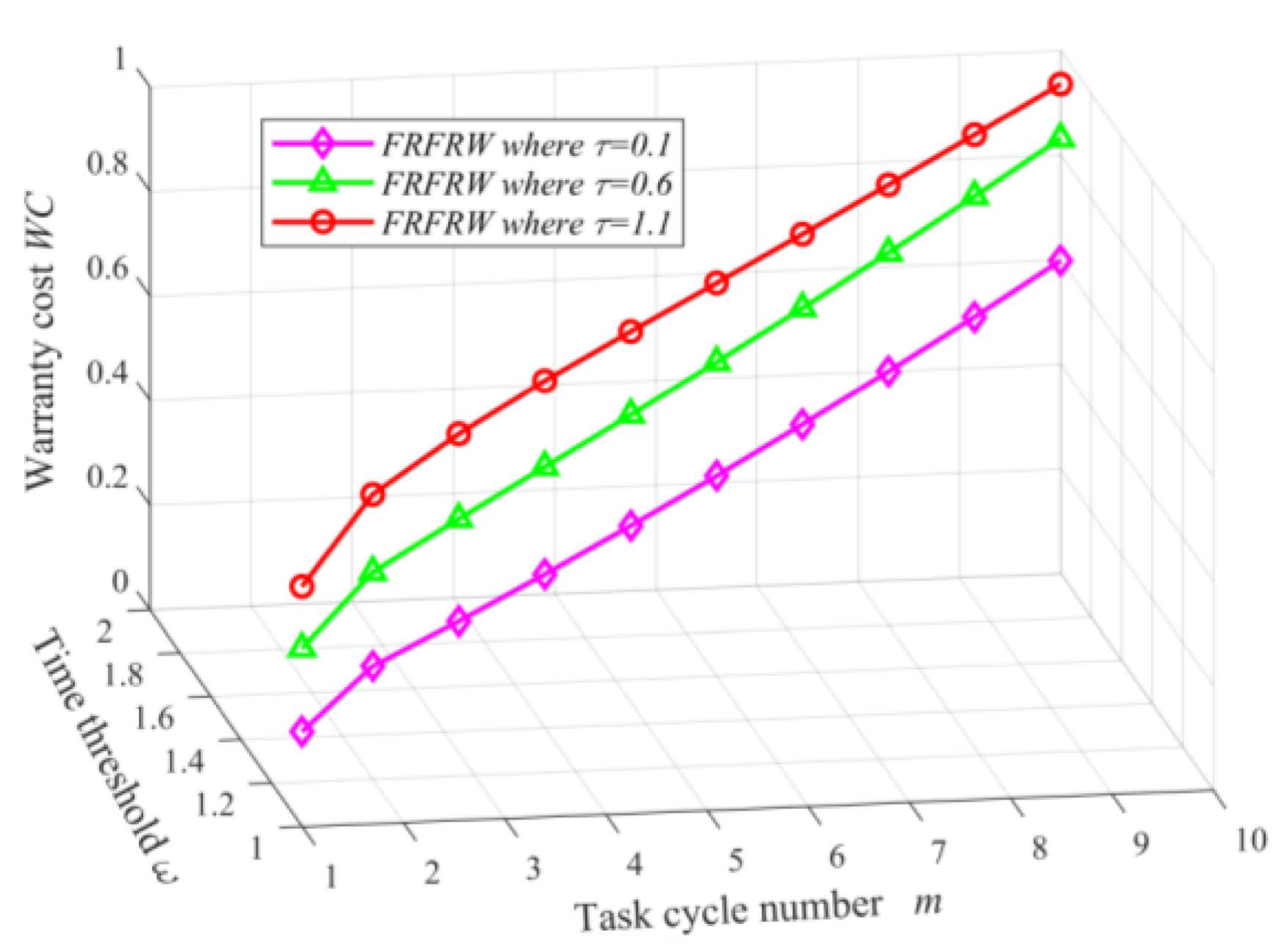
By means of
,
,
and
,
Figure 1 has been plotted to show how the time threshold
affects the warranty cost of the FRFRW. As shown in
Figure 1, given the task cycle number
and the extended time span
, the increase in the time threshold
can increase the warranty cost of the FRFRW; given the time threshold
, the increases in the extended time span
and the task cycle number
can increase the warranty cost of the FRFRW. The cause of the former is that the increase in the time threshold
can actualize the potential of triggering the service consisting of the
task cycle completing and the extended time span
; the cause of the latter is that the increases in the task cycle number
and the extended time span
extend the coverage area, which can enlarge failure frequency.
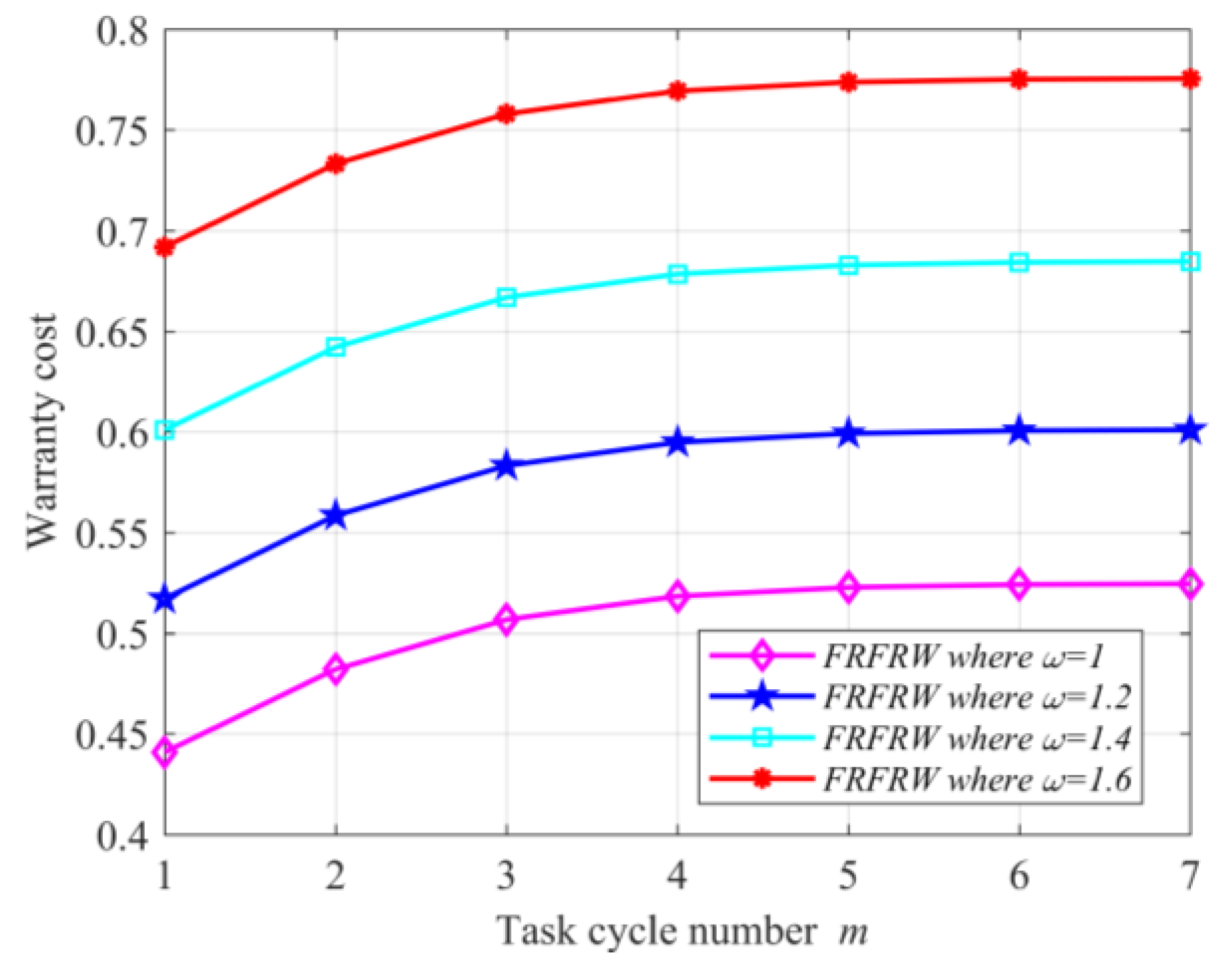
Using
,
,
and
,
Figure 2 has been offered to describe how warranty limits, i.e., the
task cycle completing or at the extended time span
, affect the warranty cost of the FRFRW. As shown in
Figure 2, the increase in the task cycle number
makes the warranty cost of the FRFRW increased to a constant, which is the warranty of the FFRW in (10); the related causes have been mentioned in the text of (10). The increase in the extended time span
increases the warranty cost of the FRFRW, and this is caused by the fact that the increase in the extended time span
must enlarge the coverage area, which can push up failure frequency.
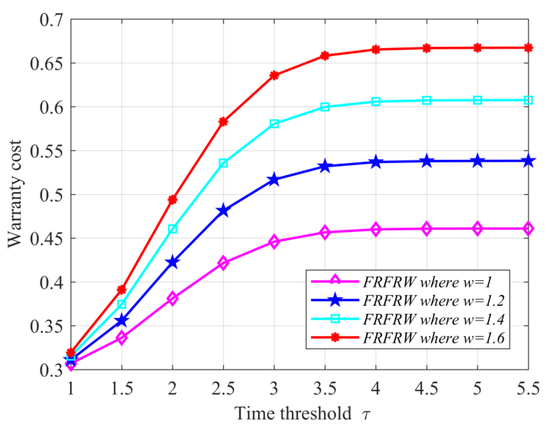
Using
,
,
and
,
Figure 3 has been offered to present how warranty limits, i.e., the time threshold
and the extended time span
, affect the warranty cost of the FRFRW. As shown in
Figure 3, the increase in the time threshold
increases the warranty cost of the FRFRW to a constant, which is the warranty cost of (8); the increase the extended time span
makes the warranty cost of the FRFRW increase, whose cause is similar to that of
in
Figure 2.
4.2. Illustration of the CRR Properties
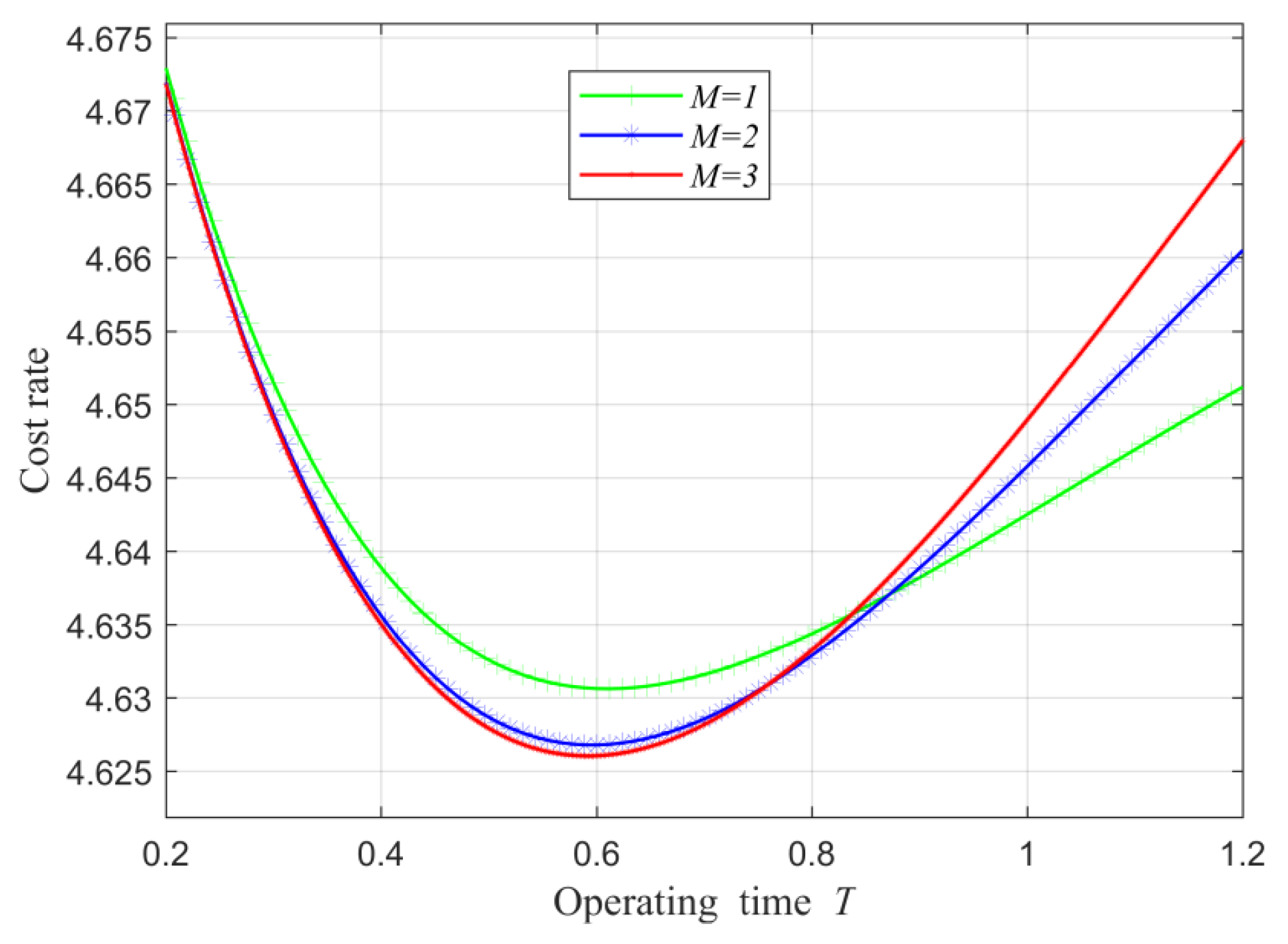
To test whether the optimal CRR exists,
Figure 4 has been offered using
,
,
,
,
,
and
.
Figure 4 shows that the optimal CRR exists uniquely when
is given, and the increase in
can decrease the minimum cost rate
and shorten the optimal operating time
. These signal that the variation in
has a homogeneous effect on both the minimum cost rate
and the optimal operating time
.
By means of
,
,
,
,
,
and
,
Table 1 has been offered to describe how the extended time span
affects the optimal CRR.
Table 1 shows that the increase in the extended time span
can decline the minimum cost rate
and reduce the optimal operating time
. These mean that the larger coverage area for warranty models must reduce the minimum cost rate
, but cannot lengthen the service life during the late stage of the through-life cycle.
By means of
,
,
,
,
,
and
,
Table 2 has been offered to describe how the extended time span
affects the optimal CRR.
Table 2 shows that the increase in the extended time span
makes the minimum cost rate
decline and the optimal operating time
shorten, which are similar to that of
Table 1 and similarly mean that the greater coverage area for warranty models must reduce the minimum cost rate
, but cannot lengthen the service life time during the late stage of the through-life cycle.
Defining
,
,
,
,
,
and
,
Table 3 has been provided to express how the extended time span
affects the optimal CRR.
Table 3 shows that the increase in the extended time span
can likewise reduce the minimum cost rate
and shorten the optimal operating time
, which are similar to that of
Table 1 and
Table 2.
Setting
,
,
,
,
and
,
Table 4 has been offered to explore how the corrective replacement cost
and the preventive replacement cost
affect the optimal CRR.
Table 4 shows that the increase in the preventive replacement cost
can increase the minimum cost rate
and lengthen the optimal operating time
; the increase in the corrective replacement cost
can enhance the minimum cost rate
and reduce the optimal operating time
.
4.3. Illustration of the CRR Performance
In
Figure 4, it has been shown that the increase in
can increase the minimum cost rate
and lengthen the optimal operating time
. These cannot illustrate the CRR performance because there exists the same transformation law for both. To illustrate the CRR performance, we present a numerical method by unifying the dimensions of the cost and time according to the same dimension, as shown below.
Let and be cycle lengths of RARF and CRR; then, the numerical method includes the following two steps:
- ①
Computing and ; where and are the denominators of (32, 32), and as well as are the numerators of (33, 32);
- ②
CRR should be selected if ; any of both can be selected if ; RARF should be selected if .
Table 5 has been offered to illustrate the CRR performance by means of
,
,
,
,
,
and
.
Table 5 shows that the cycle length with
is larger than the cycle length with
, i.e.,
. This relationship signals that the performance of the CRR is better than the performance of the RARF.
5. Conclusions
Considering that there exist differences among reliabilities of new identical products that survive the burn-in test, this study designed two random models, which can be performed one after the other to manage reliabilities during the through-life cycle from the perspectives of warrantors and warrantees. Comparing the relationship between the arrival time to the first failure and the pre-specified time threshold is used as one of the key methods to screen the differences in the reliabilities of new identical products. Based on screening results, two types of services with different coverage areas are further triggered to manage the product reliabilities during the early stage of the through-life cycle in order for warranty costs to be flexibly controlled. Due to both flexibility existence and considering minimal repair, the warranty model designed in this study was called a flexible random free repair warranty (FRFRW) model. From the perspective of reliability theory, the measures and derivatives of the FRFRW were presented to mathematically characterize all models. Similarly, a random replacement model was customized based on the relationship between the arrival time to the first failure and the pre-specified time threshold for controlling maintenance costs and lengthening service life, which was called a customized random replacement (CRR) model. The objective functions of both CRR and related derivatives are mathematically modeled to characterize them. The characteristics of some models are dissected by means of numerical analysis, which has shown that the CRR is more advantageous compared to the random age replacement first model in the published works.
In this study, two random models are designed to manage the through-life reliability by differing the reliabilities among new identical products. From the perspectives of the consumers’ usage data, product task cycles among the different consumers are heterogeneous. Therefore, a novel topic involves screening heterogeneities of task cycles to design random models that are suited to the different usage categories of task cycles. This topic is currently being investigated by authors.


