On the Simulations of Second-Order Oscillatory Problems with Applications to Physical Systems

Abstract

Second-order oscillatory problems have been found to be applicable in studying various phenomena in science and engineering; this is because these problems have the capabilities of replicating different aspects of the real world. In this research, a new hybrid method shall be formulated for the simulations of second-order oscillatory problems with applications to physical systems. The proposed method shall be formulated using the procedure of interpolation and collocation by adopting power series as basis function. In formulating the method, off-step points were introduced within the interval of integration in order to bypass the Dahlquist barrier, improve the accuracy of the method and also upgrade the order of consistence of the method. The paper further validated the some properties of the hybrid method derived and from the results obtained; the new method was found to be consistent, convergent and stable. The simulation results generated as a result of the application of the new method on some second-order oscillatory differential equations also showed that the new hybrid method is computationally reliable.

1. Introduction

Over the years, second-order differential equations with oscillatory or periodic solutions have attracted the attention of researchers. In this research, a new hybrid method is formulated for the simulations of second-order oscillatory problems (with applications to physical systems) of the form,

$$\left.\begin{array}{l}{y}^{″}(t)=\psi \left(t,y(t),y^{\prime }(t)\right)\\ y(t_0)=y_0, y^{\prime }(t_0)=y^{\prime }{}_0\end{array}\right\}$$

(1)

where $\psi :\Re \times {\Re }^{2n}\to \Re$ is a sufficiently differentiable function satisfying Theorem 1. Equations of the form (1) have been known to exhibit special properties like damping, stiffness and chaos, which make them tedious to solve [1]. In fact, some of such problems do not have closed form solution(s), thus, numerical methods have to be developed in order to approximate their solutions or at least simulate their behaviors and nature.

Theorem 1.

Ref. [2]

“Let,

$$y^{(n)}(t)=\psi \left(t, y(t), y^{\prime }(t),\dots , y^{(n-1)}(t)\right), y^{(k)}(t_0)=y_k$$

(2)

where $k=0,1,2,\dots ,(n-1)$, $y^{(0)}=y$, $y(t)$ and $\psi$ are functions defined on ${\Re }^n$, ${\Re }^n$ being a region defined by the inequalities $t_0\le t\le t_0+a, \left|s_k-y_k\right|\le b_k, k=0,1,\dots ,n-1$, where $y_k\ge 0$ for $k>0$. Let the function $\psi (t,s_0,s_1,\dots ,s_{n-1})$ in (1) be continuous, non-decreasing and non-negative in $t$, and non-decreasing and continuous in $s_k$ for $k=0,1,\dots ,n-1$ in ${\Re }^n$. Furthermore, if $\psi (t,y_0,y_1,\dots ,y_{n-1})\ne 0$ in ${\Re }^n$ for $t>t_0$, then problem (1) has at most one solution in ${\Re }^n$”.

According to [3], the influence upon or within an oscillating system that reduces, restricts or prevents its oscillation is called damping. On the other hand, simulation is the recreation of a scenario, often repeatedly, with the aid of a mathematical model, so that the likelihood of various outcomes can be more accurately estimated.

Second-order oscillatory problems have been found to be applicable in modeling physical systems in different areas of human endeavor. These areas include weak signal detection [4], projectile motion with aerodynamic drag and half cylinder rolling on a horizontal plane [5], vibrations [6,7], theory of stiffness [8], contractions [9], damping [10,11,12], phase-lags [13,14] and theory of oscillations [15,16]. Other areas of applications include special domains [17,18,19], quadrotor flight control [20], rings [21], dynamical systems [22] and epidemic models [23].

Some scholars proposed methods for the solutions and simulations of second order oscillatory problems. These methods among others are Laplace decomposition algorithm [24], Adomian decomposition method [25], Taylor matrix method [26], differential transform method [27,28], variational iteration method [29,30,31], Runge-Kutta method [32] and hybrid block methods [33,34,35,36,37,38,39,40]. The authors in [41] for instance, developed hybrid method for solving second order problems while [42] proposed an accuracy-preserving algorithm of order six, for integrating second order oscillatory problems. Suffice to mention that some of these methods have some disadvantages like low rate of convergence, large number of function evaluation per step, low order of accuracy, non-flexibility in terms of step size change, among others.

It is in view of the setbacks highlighted above, that a continuous hybrid method with fewer function evaluations, higher order of accuracy and high rate of convergence is proposed in this research. The proposed method is also easy to program and is efficient with respect to economy of computer time.

Definition 1.

(Hybrid Method)

“A linear multistep method is called hybrid if off-grid point(s) is/are incorporated between conventional points within integration interval.”

2. Main Method

2.1. Derivation of the Method

The derivation of a new method for simulations of oscillatory second-order problems is carried out in this section. The method which shall be derived is of the form,

$$A^{(0)}{Y}_m^{(i)}={\displaystyle \sum _{i=0}^{1-i}{h}^i{e}_i{y}_n^{(i)}}+h^{\mu -i}\left[d_{i}f(y_n)+b_{i}f(Y_m)\right]$$

(3)

where

$$\begin{gathered} Y_m^{(i)}={\left[y_{n+i}^{(i)} y_{n+j}^{(i)} \dots y_{n+1}^{(i)}\right]}^T, f(Y_m)={\left[f_{n+i} f_{n+j} \dots f_{n+1}\right]}^T \\ {y}_n^{(i)}={\left[y_{n-i}^{(i)} y_{n-j}^{(i)} \dots y_n^{(i)}\right]}^T, f(y_n)={\left[f_{n-i} f_{n-j} \dots f_n\right]}^T \end{gathered}$$

$A^{(0)}=(\omega -1)\times (\omega -1)$ is an identity matrix, $\mu$ is the differential equation’s order, and $(i)$ is the power of derivative of the method. Note that $h$ is the step-size calculated as $h=t_{n+1}-t_n$, $n=0,1,2,\dots ,N$. The oscillatory problem (1) is solved in the $N$ non-overlapping blocks.

At $i=0$, the $(\omega -1)\times (\omega -1)$ matrices $e_0,e_1,d_0$ and $b_0$ are evaluated and at $i=1$ (the first derivative), the $(\omega -1)\times (\omega -1)$ matrices $e_1,d_1$ and $b_1$ are evaluated. Let the computed solution of the oscillatory problem (1) be approximated by the power series

$$y(t)={\displaystyle \sum _{j=0}^{\omega +\tau -1}{\upsilon }_j{t}^j}$$

(4)

The condition $\omega +\tau$ (where $\omega$ is the number of collocation points and $\tau$ is the number of interpolation points) is then imposed on Equation (4), which gives the polynomials of degree $m=\omega +\tau -1$ (at most) as follows

$$y(t_{n+{\tau }_1})=y_{n+{\tau }_1}={\displaystyle \sum _{j=0}^{\omega +\tau -1}{\upsilon }_j{t}_{n+{\tau }_1}^j}$$

(5)

$$y(t_{n+{\tau }_2})=y_{n+{\tau }_2}={\displaystyle \sum _{j=0}^{\omega +\tau -1}{\upsilon }_j{t}_{n+{\tau }_2}^j}$$

(6)

$$y^{″}(t_{n+\kappa })=f_{n+\kappa }={\displaystyle \sum _{j=0}^{\omega +\tau -1}j(j-1){\upsilon }_j{t}_{n+\kappa }^{j-2}}$$

(7)

where $\kappa =\left(0,p,q,r,s,u,w,1\right)=\left(0,1/7, 2/7, 3/7, 4/7, 5/7, 6/7, 1\right)$ and $\left[{\tau }_1,{\tau }_2\right]=\left[\frac{5}{7},\frac{6}{7}\right]$. This leads to a system of $\omega +\tau$ equations each of degree at most $m$ which is written compactly in matrix form as

$$TV=U$$

(8)

where

$$\begin{gathered} V=\left[{\upsilon }_0 {\upsilon }_1 {\upsilon }_2 \dots {\upsilon }_9 \right] \\ U={\left[y_{n+{\tau }_1} y_{n+{\tau }_2} f_n f_{n+p} f_{n+q} f_{n+r} f_{n+s} f_{n+u} f_{n+w} f_{n+1}\right]}^T \end{gathered}$$

and

$$T=\left[\begin{array}{llllllllll}1& t_{n+{\tau }_1}& t_{n+{\tau }_1}^2& t_{n+{\tau }_1}^3& t_{n+{\tau }_1}^4& t_{n+{\tau }_1}^5& t_{n+{\tau }_1}^6& t_{n+{\tau }_1}^7& t_{n+{\tau }_1}^8& t_{n+{\tau }_1}^9\\ 1& t_{n+{\tau }_2}& t_{n+{\tau }_2}^2& t_{n+{\tau }_2}^3& t_{n+{\tau }_2}^4& t_{n+{\tau }_2}^5& t_{n+{\tau }_2}^6& t_{n+{\tau }_2}^7& t_{n+{\tau }_2}^8& t_{n+{\tau }_2}^9\\ 0& 0& 2& 6t_n& 12t_n^2& 20t_n^3& 30t_n^4& 42t_n^5& 56t_n^6& 72t_n^7 \\ 0& 0& 2& 6t_{n+p}& 12t_{n+p}^2& 20t_{n+p}^3& 30t_{n+p}^4& 42t_{n+p}^5& 56t_{n+p}^6& 72t_{n+p}^7 \\ 0& 0& 2& 6t_{n+q}& 12t_{n+q}^2& 20t_{n+q}^3& 30t_{n+q}^4& 42t_{n+q}^5& 56t_{n+q}^6& 72t_{n+q}^7 \\ 0& 0& 2& 6t_{n+r}& 12t_{n+r}^2& 20t_{n+r}^3& 30t_{n+r}^4& 42t_{n+r}^5& 56t_{n+r}^6& 72t_{n+r}^7\\ 0& 0& 2& 6t_{n+s}& 12t_{n+s}^2& 20t_{n+s}^3& 30t_{n+s}^4& 42t_{n+s}^5& 56t_{n+s}^6& 72t_{n+s}^7\\ 0& 0& 2& 6t_{n+u}& 12t_{n+u}^2& 20t_{n+u}^3& 30t_{n+u}^4& 42t_{n+u}^5& 56t_{n+u}^6& 72t_{n+u}^7\\ 0& 0& 2& 6t_{n+w}& 12t_{n+w}^2& 20t_{n+w}^3& 30t_{n+w}^4& 42t_{n+w}^5& 56t_{n+w}^6& 72t_{n+w}^7\\ 0& 0& 2& 6t_{n+1}& 12t_{n+1}^2& 20t_{n+1}^3& 3 0t_{n+1}^4& 42t_{n+1}^5& 56t_{n+1}^6& 72t_{n+1}^7\end{array}\right]$$

Equation (8) is then solved using the Gaussian elimination method for all the ${\upsilon }_j{}^{\prime }s$ which are parameters to be determined. These parameters are inputted into Equation (4) to give the continuous hybrid method

$$y(t)={\displaystyle \sum _{\tau ={\tau }_1,{\tau }_2}{\alpha }_{\tau }(t)y_{n+\tau }}+h^2\left({\displaystyle \sum _{j=0}^1{\beta }_j(t)f_{n+j}+{\beta }_{\kappa }(t)f_{n+\kappa }}\right), \kappa =p,q,r,s,u,w$$

(9)

where

$$\left.\begin{array}{l}{\alpha }_{{\tau }_1}(x)=6-7x\\ {\alpha }_{{\tau }_2}(x)=7x-5\\ \begin{array}{l}{\beta }_0(x)=-\frac{1}{88905600}\left(\begin{array}{l}201768035x^9-1037664180x^8+2272978680x^7\\ -2767104480x^6+2047798494x^5-945897960x^4\\ +268939440x^3-44452800x^2+3739561x-110490\end{array}\right)\\ {\beta }_p(x)=\frac{1}{88905600}\left(\begin{array}{l}1412376245x^9-7004233215x^8+14576711100x^7\\ -16454389140x^6+10808648928x^5-4047797880x^4\\ +726062400x^3-19424888x+1999920\end{array}\right)\\ {\beta }_q(x)=-\frac{1}{29635200}\left(\begin{array}{l}1412376245x^9-6744817170x^8+13341396600x^7\\ -14033172720x^6+8320372578x^5-2659203540x^4\\ +363031200x^3+1034257x-1073130\end{array}\right)\\ {\beta }_r(x)=\frac{1}{17781120}\left(\begin{array}{l}1412376245x^9-6485401125x^8+12204907260x^7\\ -12046787004x^6+6590226384x^5-1913981160x^4\\ +242020800x^3-4634042x+1203780\end{array}\right)\\ {\beta }_s(x)=-\frac{1}{17781120}\left(\begin{array}{l}1412376245x^9-6225985080x^8+11167243080x^7\\ -10435936896x^6+5389500690x^5-1488427920x^4\\ +181515600x^3+979363x-1352670\end{array}\right)\\ {\beta }_u(x)=\frac{1}{29635200}\left(\begin{array}{l}1412376245x^9-5966569035x^8+10228404060x^7\\ -9141327300x^6+4540310208x^5-1216154520x^4\\ +145212480x^3-5101628x+2786520\end{array}\right)\\ {\beta }_w(x)=-\frac{1}{88905600}\left(\begin{array}{l}1412376245x^9-5707152990x^8+9388390200x^7\\ -8103663120x^6+3915594018x^5-1027579980x^4\\ +121010400x^3+130837x-765330\end{array}\right)\\ {\beta }_1(x)=\frac{1}{88905600}\left(\begin{array}{l}201768035x^9-778248135x^8+1235314500x^7\\ -1037664180x^6+491302224x^5-127060920x^4\\ +14817600x^3-84434x-20940\end{array}\right)\end{array}\end{array}\right\}$$

(10)

 and $x$ is given by the expression

$$x=\frac{t-t_n}{h}$$

(11)

Equation (9) is solved for the independent solution at $f_{n+j}$ and $f_{n+\kappa }$ to obtain the continuous hybrid method

$$Y_{n+j}={\displaystyle \sum _{i=0}^1\frac{{(jh)}^i}{i !}{y}_n^{(i)}+h^2\left({\displaystyle \sum _{j=0}^1{\sigma }_j(t)f_{n+j}+{\sigma }_{\kappa }(t)f_{n+\kappa }}\right), \kappa =p,q,r,s,u,w}$$

(12)

where $f_{n+j}$ and $f_{n+\kappa }$ have the following coefficients,

$$\left.\begin{array}{l}{\sigma }_0(x)=-\frac{1}{17280}\left(\begin{array}{l}352947x^8-1613472x^7+3092488x^6-3226944x^5\\ +1990086x^4-735392x^3+156816x^2-17280x\end{array}\right)\\ {\sigma }_p(x)=\frac{49}{17280}\left(\begin{array}{l}50421x^8-222264x^7+404740x^6-391608x^5\\ +214368x^4-64224x^3+8640x^2\end{array}\right)\\ {\sigma }_q(x)=-\frac{49}{1920}\left(\begin{array}{l}16807x^8-71344x^7+123480x^6-111328x^5\\ +55006x^4-14064x^3+1440x^2\end{array}\right)\\ {\sigma }_r(x)=\frac{49}{17280}\left(\begin{array}{l}252105x^8-1029000x^7+1694420x^6-1433544x^5\\ +653520x^4-151840x^3+14400x^2\end{array}\right)\\ {\sigma }_s(x)=-\frac{49}{17280}\left(\begin{array}{l}252105x^8-987840x^7+1550360x^6-1241856x^5\\ +534450x^4-118080x^3+10800x^2\end{array}\right)\\ {\sigma }_u(x)=\frac{49}{1920}\left(\begin{array}{l}16807x^8-63112x^7+94668x^6-72520x^5\\ +30016x^4-6432x^3+576x^2\end{array}\right)\\ {\sigma }_w(x)=-\frac{49}{17280}\left(\begin{array}{l}50421x^8-181104x^7+260680x^6-192864x^5\\ +77658x^4-16304x^3+1440x^2\end{array}\right)\\ {\sigma }_1(x)=\frac{1}{17280}\left(\begin{array}{l}352947x^8-1210104x^7+1680700x^6-1210104x^5\\ +477456x^4-98784x^3+8640x^2\end{array}\right)\end{array}\right\}$$

(13)

Evaluating (12) at $t=p,q,r,s,u,w,1$ produces discrete hybrid scheme of the form (3) where

$$\begin{gathered} Y_m^{(i)}={\left[y_{n+\frac{1}{7}}^{(i)} y_{n+\frac{2}{7}}^{(i)} y_{n+\frac{3}{7}}^{(i)} y_{n+\frac{4}{7}}^{(i)} y_{n+\frac{5}{7}}^{(i)} y_{n+\frac{6}{7}}^{(i)} y_1^{(i)}\right]}^T \\ {y}_n^{(i)}={\left[y_{n-\frac{1}{7}}^{(i)} y_{n-\frac{2}{7}}^{(i)} y_{n-\frac{3}{7}}^{(i)} y_{n-\frac{4}{7}}^{(i)} y_{n-\frac{5}{7}}^{(i)} y_{n-\frac{6}{7}}^{(i)} y_n^{(i)}\right]}^T \\ F(Y_m)={\left[f_{n+\frac{1}{7}} f_{n+\frac{2}{7}} f_{n+\frac{3}{7}} f_{n+\frac{4}{7}} f_{n+\frac{5}{7}} f_{n+\frac{6}{7}} f_1\right]}^T \\ f(y_n)={\left[f_{n-\frac{1}{7}} f_{n-\frac{2}{7}} f_{n-\frac{3}{7}} f_{n-\frac{4}{7}} f_{n-\frac{5}{7}} f_{n-\frac{6}{7}} f_n\right]}^T \end{gathered}$$

$A^{(0)}$ is an identity matrix of dimension $7\times 7$ given by

$$A^{(0)}=\left[\begin{array}{l}1 0 0 0 0 0 0\\ 0 1 0 0 0 0 0\\ 0 0 1 0 0 0 0\\ 0 0 0 1 0 0 0\\ 0 0 0 0 1 0 0\\ 0 0 0 0 0 1 0\\ 0 0 0 0 0 0 1\end{array}\right]$$

At $i=0$, we obtain

$$\begin{gathered} e_0=\left[\begin{array}{l}0 0 0 0 0 0 1\\ 0 0 0 0 0 0 1\\ 0 0 0 0 0 0 1\\ 0 0 0 0 0 0 1\\ 0 0 0 0 0 0 1\\ 0 0 0 0 0 0 1\\ 0 0 0 0 0 0 1\end{array}\right], e_1=\left[\begin{array}{l}0 0 0 0 0 0 \frac{1}{7}\\ 0 0 0 0 0 0 \frac{2}{7}\\ 0 0 0 0 0 0 \frac{3}{7}\\ 0 0 0 0 0 0 \frac{4}{7}\\ 0 0 0 0 0 0 \frac{5}{7}\\ 0 0 0 0 0 0 \frac{6}{7}\\ 0 0 0 0 0 0 1\end{array}\right] \\ {d}_0=\left[\begin{array}{l}0 0 0 0 0 0 \frac{416173}{88905600}\\ 0 0 0 0 0 0 \frac{14939}{1389150}\\ 0 0 0 0 0 0 \frac{18399}{1097600}\\ 0 0 0 0 0 0 \frac{15824}{694575}\\ 0 0 0 0 0 0 \frac{102425}{3556224}\\ 0 0 0 0 0 0 \frac{597}{17150}\\ 0 0 0 0 0 0 \frac{10597}{259200}\end{array}\right] \end{gathered}$$

$$b_0=\left[\begin{array}{lllllll}\frac{33953}{3175200}& -\frac{341699}{29635200}& \frac{105943}{8890560}& -\frac{153761}{17781120}& \frac{943}{231525}& -\frac{99359}{88905600}& \frac{6031}{44452800}\\ \frac{27821}{694575}& -\frac{17}{675}& \frac{799}{27783}& -\frac{5881}{277830}& \frac{2321}{231525}& -\frac{1916}{694575}& \frac{233}{694575}\\ \frac{39141}{548800}& -\frac{24111}{1097600}& \frac{369}{7840}& -\frac{7299}{219520}& \frac{8613}{548800}& -\frac{4737}{1097600}& \frac{9}{17150}\\ \frac{71152}{694575}& -\frac{3832}{231525}& \frac{11344}{138915}& -\frac{856}{19845}& \frac{4912}{231525}& -\frac{4072}{694575}& \frac{496}{694575}\\ \frac{59375}{444528}& -\frac{13375}{1185408}& \frac{210625}{1778112}& -\frac{130625}{3556224}& \frac{25}{864}& -\frac{26875}{3556224}& \frac{1625}{1778112}\\ \frac{1413}{8575}& -\frac{54}{8575}& \frac{267}{1715}& -\frac{99}{3430}& \frac{459}{8575}& -\frac{9}{1225}& \frac{9}{8575}\\ \frac{25333}{129600}& \frac{49}{86400}& \frac{245}{1296}& -\frac{833}{51840}& \frac{3283}{43200}& \frac{2989}{259200}& \frac{167}{64800}\end{array}\right]$$

At $i=1$, we obtain

$$e_1=\left[\begin{array}{l}0 0 0 0 0 0 1\\ 0 0 0 0 0 0 1\\ 0 0 0 0 0 0 1\\ 0 0 0 0 0 0 1\\ 0 0 0 0 0 0 1\\ 0 0 0 0 0 0 1\\ 0 0 0 0 0 0 1\end{array}\right], d_1=\left[\begin{array}{l}0 0 0 0 0 0 \frac{751}{17280}\\ 0 0 0 0 0 0 \frac{41}{980} \\ 0 0 0 0 0 0 \frac{265}{6272} \\ 0 0 0 0 0 0 \frac{278}{6615} \\ 0 0 0 0 0 0 \frac{265}{6272}\\ 0 0 0 0 0 0 \frac{41}{980}\\ 0 0 0 0 0 0 \frac{751}{17280}\end{array}\right]$$

$$b_1=\left[\begin{array}{lllllll}\frac{139849}{846720}& -\frac{4511}{31360}& \frac{123133}{846720}& -\frac{88547}{846720}& \frac{1537}{31360}& -\frac{11351}{846720}& \frac{275}{169344}\\ \frac{1466}{6615}& -\frac{71}{2940}& \frac{68}{735}& -\frac{1927}{26460}& \frac{26}{735}& -\frac{29}{2940}& \frac{8}{6615}\\ \frac{1359}{6272}& \frac{1377}{31360}& \frac{5927}{31360}& -\frac{3033}{31360}& \frac{1377}{31360}& -\frac{373}{31360}& \frac{9}{6272}\\ \frac{1448}{6615}& \frac{8}{245}& \frac{1784}{6615}& -\frac{106}{6615}& \frac{8}{245}& -\frac{64}{6615}& \frac{8}{6615}\\ \frac{36725}{169344}& \frac{775}{18816}& \frac{4625}{18816}& \frac{13625}{169344}& \frac{1895}{18816}& -\frac{275}{18816}& \frac{275}{169344}\\ \frac{54}{245}& \frac{27}{980}& \frac{68}{245}& \frac{27}{980}& \frac{54}{245}& \frac{41}{980}& 0\\ \frac{3577}{17280}& \frac{49}{640}& \frac{2989}{17280}& \frac{2989}{17280}& \frac{49}{640}& \frac{3577}{17280}& \frac{751}{17280}\end{array}\right]$$

The proposed hybrid method is thus given by,

$$\left.\begin{array}{l}{y}_{n+\frac{1}{7}}=y_n+\frac{1}{7}h{y}_n^{\prime }+h^2\left(\begin{array}{l}\frac{416173}{88905600}{f}_n+\frac{33953}{3175200}{f}_{n+\frac{1}{7}}-\frac{341699}{29635200}{f}_{n+\frac{2}{7}}+\frac{105943}{8890560}{f}_{n+\frac{3}{7}}\\ -\frac{153761}{17781120}{f}_{n+\frac{4}{7}}+\frac{943}{231525}{f}_{n+\frac{5}{7}}-\frac{99359}{88905600}{f}_{n+\frac{6}{7}}+\frac{6031}{44452800}{f}_{n+1}\end{array}\right)\\ y_{n+\frac{2}{7}}=y_n+\frac{2}{7}h{y}_n^{\prime }+h^2\left(\begin{array}{l}\frac{14939}{1389150}{f}_n+\frac{27821}{694575}{f}_{n+\frac{1}{7}}-\frac{17}{675}{f}_{n+\frac{2}{7}}+\frac{799}{27783}{f}_{n+\frac{3}{7}}\\ -\frac{5881}{277830}{f}_{n+\frac{4}{7}}+\frac{2321}{231525}{f}_{n+\frac{5}{7}}-\frac{1916}{694575}{f}_{n+\frac{6}{7}}+\frac{233}{694575}{f}_{n+1}\end{array}\right)\\ y_{n+\frac{3}{7}}=y_n+\frac{3}{7}h{y}_n^{\prime }+h^2\left(\begin{array}{l}\frac{18399}{1097600}{f}_n+\frac{39141}{54880}{f}_{n+\frac{1}{7}}-\frac{24111}{1097600}{f}_{n+\frac{2}{7}}+\frac{369}{7840}{f}_{n+\frac{3}{7}}\\ -\frac{7299}{219520}{f}_{n+\frac{4}{7}}+\frac{8613}{548800}{f}_{n+\frac{5}{7}}-\frac{4737}{1097600}{f}_{n+\frac{6}{7}}+\frac{9}{17150}{f}_{n+1}\end{array}\right)\\ y_{n+\frac{4}{7}}=y_n+\frac{4}{7}h{y}_n^{\prime }+h^2\left(\begin{array}{l}\frac{15824}{694575}{f}_n+\frac{71152}{694575}{f}_{n+\frac{1}{7}}-\frac{3832}{231525}{f}_{n+\frac{2}{7}}+\frac{11344}{138915}{f}_{n+\frac{3}{7}}\\ -\frac{856}{19845}{f}_{n+\frac{4}{7}}+\frac{4912}{231525}{f}_{n+\frac{5}{7}}-\frac{4072}{694575}{f}_{n+\frac{6}{7}}+\frac{496}{694575}{f}_{n+1}\end{array}\right)\\ y_{n+\frac{5}{7}}=y_n+\frac{5}{7}h{y}_n^{\prime }+h^2\left(\begin{array}{l}\frac{102425}{3556224}{f}_n+\frac{59375}{444528}{f}_{n+\frac{1}{7}}-\frac{13375}{1185408}{f}_{n+\frac{2}{7}}+\frac{210625}{1778112}{f}_{n+\frac{3}{7}}\\ -\frac{130625}{3556224}{f}_{n+\frac{4}{7}}+\frac{25}{864}{f}_{n+\frac{5}{7}}-\frac{26875}{3556224}{f}_{n+\frac{6}{7}}+\frac{1625}{1778112}{f}_{n+1}\end{array}\right)\\ y_{n+\frac{6}{7}}=y_n+\frac{6}{7}h{y}_n^{\prime }+h^2\left(\begin{array}{l}\frac{597}{17150}{f}_n+\frac{1413}{8575}{f}_{n+\frac{1}{7}}-\frac{54}{8575}{f}_{n+\frac{2}{7}}+\frac{267}{1715}{f}_{n+\frac{3}{7}}\\ -\frac{99}{3430}{f}_{n+\frac{4}{7}}+\frac{459}{8575}{f}_{n+\frac{5}{7}}-\frac{9}{1225}{f}_{n+\frac{6}{7}}+\frac{9}{8575}{f}_{n+1}\end{array}\right)\\ y_{n+1}=y_n+h{y}_n^{\prime }+h^2\left(\begin{array}{l}\frac{10597}{259200}{f}_n+\frac{25333}{129600}{f}_{n+\frac{1}{7}}+\frac{49}{86400}{f}_{n+\frac{2}{7}}+\frac{245}{1296}{f}_{n+\frac{3}{7}}\\ -\frac{833}{51840}{f}_{n+\frac{4}{7}}+\frac{3283}{43200}{f}_{n+\frac{5}{7}}+\frac{2989}{259200}{f}_{n+\frac{6}{7}}+\frac{167}{64800}{f}_{n+1}\end{array}\right)\end{array}\right\}$$

(14)

and

$$\left.\begin{array}{l}{y}_{n+\frac{1}{7}}^{\prime }=y_n^{\prime }+h\left(\begin{array}{l}\frac{751}{17280}{f}_n+\frac{139849}{8467720}{f}_{n+\frac{1}{7}}-\frac{4511}{31360}{f}_{n+\frac{2}{7}}+\frac{123133}{846720}{f}_{n+\frac{3}{7}}\\ -\frac{88547}{846720}{f}_{n+\frac{4}{7}}+\frac{1537}{31360}{f}_{n+\frac{5}{7}}-\frac{11351}{846720}{f}_{n+\frac{6}{7}}+\frac{275}{169344}{f}_{n+1}\end{array}\right)\\ y_{n+\frac{2}{7}}^{\prime }=y_n^{\prime }+h\left(\begin{array}{l}\frac{41}{980}{f}_n+\frac{1466}{6615}{f}_{n+\frac{1}{7}}-\frac{71}{2940}{f}_{n+\frac{2}{7}}+\frac{68}{735}{f}_{n+\frac{3}{7}}\\ -\frac{1927}{26460}{f}_{n+\frac{4}{7}}+\frac{26}{735}{f}_{n+\frac{5}{7}}-\frac{29}{2940}{f}_{n+\frac{6}{7}}+\frac{8}{6615}{f}_{n+1}\end{array}\right)\\ y_{n+\frac{3}{7}}^{\prime }=y_n^{\prime }+h\left(\begin{array}{l}\frac{265}{6272}{f}_n+\frac{1359}{6272}{f}_{n+\frac{1}{7}}+\frac{1377}{31360}{f}_{n+\frac{2}{7}}+\frac{5927}{31360}{f}_{n+\frac{3}{7}}\\ -\frac{3033}{31360}{f}_{n+\frac{4}{7}}+\frac{1377}{31360}{f}_{n+\frac{5}{7}}-\frac{373}{31360}{f}_{n+\frac{6}{7}}+\frac{9}{6272}{f}_{n+1}\end{array}\right)\\ y_{n+\frac{4}{7}}^{\prime }=y_n^{\prime }+h\left(\begin{array}{l}\frac{278}{6615}{f}_n+\frac{1448}{6615}{f}_{n+\frac{1}{7}}+\frac{8}{245}{f}_{n+\frac{2}{7}}+\frac{1784}{6615}{f}_{n+\frac{3}{7}}\\ -\frac{106}{6615}{f}_{n+\frac{4}{7}}+\frac{8}{245}{f}_{n+\frac{5}{7}}-\frac{64}{6615}{f}_{n+\frac{6}{7}}+\frac{8}{6615}{f}_{n+1}\end{array}\right)\\ y_{n+\frac{5}{7}}^{\prime }=y_n^{\prime }+h\left(\begin{array}{l}\frac{265}{6272}{f}_n+\frac{36725}{169344}{f}_{n+\frac{1}{7}}+\frac{775}{18816}{f}_{n+\frac{2}{7}}+\frac{4625}{18816}{f}_{n+\frac{3}{7}}\\ +\frac{13625}{169344}{f}_{n+\frac{4}{7}}+\frac{1895}{18816}{f}_{n+\frac{5}{7}}-\frac{275}{18816}{f}_{n+\frac{6}{7}}+\frac{275}{169344}{f}_{n+1}\end{array}\right)\\ y_{n+\frac{6}{7}}^{\prime }=y_n^{\prime }+h\left(\begin{array}{l}\frac{41}{980}{f}_n+\frac{54}{245}{f}_{n+\frac{1}{7}}+\frac{27}{980}{f}_{n+\frac{2}{7}}+\frac{68}{245}{f}_{n+\frac{3}{7}}\\ +\frac{27}{980}{f}_{n+\frac{4}{7}}+\frac{54}{245}{f}_{n+\frac{5}{7}}+\frac{41}{980}{f}_{n+\frac{6}{7}}+(0)f_{n+1}\end{array}\right)\\ y_{n+1}^{\prime }=y_n^{\prime }+h\left(\begin{array}{l}\frac{751}{17280}{f}_n+\frac{3577}{17280}{f}_{n+\frac{1}{7}}+\frac{49}{640}{f}_{n+\frac{2}{7}}+\frac{2989}{17280}{f}_{n+\frac{3}{7}}\\ +\frac{2989}{17280}{f}_{n+\frac{4}{7}}+\frac{49}{640}{f}_{n+\frac{5}{7}}+\frac{3577}{17280}{f}_{n+\frac{6}{7}}+\frac{751}{17280}{f}_{n+1}\end{array}\right)\end{array}\right\}$$

(15)

Equations (14) and (15) are simultaneously applied as the proposed method for simulating second order oscillatory problems with applications to physical systems.

2.2. Implementation of the Method

The newly derived hybrid method is self-starting, unlike the conventional predictor-corrector methods. It is implemented in block mode over a non-overlapping one-step interval $\left[t_n, t_{n+1}\right]$, with $n=0,1,2,3,\dots ,N-1$. Set data inputs like initial conditions, step size and differential equation to be solved. Thus at $n=0,$ the hybrid method is employed concurrently on the subinterval $\left[t_0,t_1\right]$ to get ${\left[y_{{\kappa }_i},y_{{\kappa }_i}^{\prime }\right]}^T$, $i=1,2,\dots 5$. Applying the values of the known former block, we get the values of the next subinterval $\left[t_1,t_2\right]$ and the process goes on in this manner until the final subinterval $\left[t_{N-1},t_N\right]$ is determined.

3. Theoretical Analysis of the Method

Special properties of the proposed hybrid method will be analyzed theoretically in this section. These properties include zero-stability, consistency, convergence order, error constant and region of absolute stability. These are properties that a numerical method is expected to satisfy for such a method to be computationally reliable.

3.1. Order and Error Constant

The linear operator related to the newly derived hybrid method is established in this subsection.

Proposition 1.

The newly derived hybrid method has local truncation error $c_{10}{h}^{10}{y}^{(10)}\left(t_n\right)+O\left(h^{11}\right)$.

Proof. 

The linear difference operators associated with the hybrid method (14) and (15) are defined as

$$\left.\begin{array}{l}{\ell }_p\left[y(t_n);h\right]=y\left(t_n+ph\right)-\left({\alpha }_{{\tau }_1}(t)y\left(t_n+{\tau }_{1}h\right)+{\alpha }_{{\tau }_2}(t)y\left(t_n+{\tau }_{2}h\right)+h^2{\displaystyle \sum _{j=0}^1\left({\beta }_j(t)f_{n+j}+{\beta }_{\kappa }(t)f_{n+\kappa }\right)}\right),\kappa =p,q,r,s,u,w\\ {\ell }_q\left[y(t_n);h\right]=y\left(t_n+qh\right)-\left({\alpha }_{{\tau }_1}(t)y\left(t_n+{\tau }_{1}h\right)+{\alpha }_{{\tau }_2}(t)y\left(t_n+{\tau }_{2}h\right)+h^2{\displaystyle \sum _{j=0}^1\left({\beta }_j(t)f_{n+j}+{\beta }_{\kappa }(t)f_{n+\kappa }\right)}\right),\kappa =p,q,r,s,u,w\\ {\ell }_r\left[y(t_n);h\right]=y\left(t_n+rh\right)-\left({\alpha }_{{\tau }_1}(t)y\left(t_n+{\tau }_{1}h\right)+{\alpha }_{{\tau }_2}(t)y\left(t_n+{\tau }_{2}h\right)+h^2{\displaystyle \sum _{j=0}^1\left({\beta }_j(t)f_{n+j}+{\beta }_{\kappa }(t)f_{n+\kappa }\right)}\right),\kappa =p,q,r,s,u,w\\ {\ell }_s\left[y(t_n);h\right]=y\left(t_n+sh\right)-\left({\alpha }_{{\tau }_1}(t)y\left(t_n+{\tau }_{1}h\right)+{\alpha }_{{\tau }_2}(t)y\left(t_n+{\tau }_{2}h\right)+h^2{\displaystyle \sum _{j=0}^1\left({\beta }_j(t)f_{n+j}+{\beta }_{\kappa }(t)f_{n+\kappa }\right)}\right),\kappa =p,q,r,s,u,w\\ {\ell }_u\left[y(t_n);h\right]=y\left(t_n+uh\right)-\left({\alpha }_{{\tau }_1}(t)y\left(t_n+{\tau }_{1}h\right)+{\alpha }_{{\tau }_2}(t)y\left(t_n+{\tau }_{2}h\right)+h^2{\displaystyle \sum _{j=0}^1\left({\beta }_j(t)f_{n+j}+{\beta }_{\kappa }(t)f_{n+\kappa }\right)}\right),\kappa =p,q,r,s,u,w\\ {\ell }_w\left[y(t_n);h\right]=y\left(t_n+wh\right)-\left({\alpha }_{{\tau }_1}(t)y\left(t_n+{\tau }_{1}h\right)+{\alpha }_{{\tau }_2}(t)y\left(t_n+{\tau }_{2}h\right)+h^2{\displaystyle \sum _{j=0}^1\left({\beta }_j(t)f_{n+j}+{\beta }_{\kappa }(t)f_{n+\kappa }\right)}\right),\kappa =p,q,r,s,u,w\\ {\ell }_1\left[y(t_n);h\right]=y\left(t_n+h\right)-\left({\alpha }_{{\tau }_1}(t)y\left(t_n+{\tau }_{1}h\right)+{\alpha }_{{\tau }_2}(t)y\left(t_n+{\tau }_{2}h\right)+h^2{\displaystyle \sum _{j=0}^1\left({\beta }_j(t)f_{n+j}+{\beta }_{\kappa }(t)f_{n+\kappa }\right)}\right),\kappa =p,q,r,s,u,w\end{array}\right\}$$

(16)

Assuming $y(t)$ is sufficiently differentiable; Equation (16) is expanded in power of $h$ with the aid of Taylor series. It is important to state that the first non-zero term of each formula in Equation (16) is $c_{10}{h}^{10}{y}^{(10)}\left(t_n\right)+O\left(h^{11}\right)$. The same procedure applies to the derivative scheme in Equation (15). $\square$

Definition 2.

Ref. [43]

“A linear multistep method for a second order problem is of order $p$ if it satisfies  $c_0$ =  $c_1$ =  $c_2$ =  $c_3$ = … =  $c_p$ =  $c_{p+1}$ =  $0,$ $c_{p+2}\ne 0$, where,

$$\left.\begin{array}{l}{c}_0={\displaystyle \sum _{j=0}^k{\alpha }_j}\\ c_1={\displaystyle \sum _{j=0}^k\left(j{\alpha }_j-{\beta }_j\right)}\\ .\\ .\\ .\\ c_p={\displaystyle \sum _{j=0}^k\left[\frac{1}{p!}{j}^p{\alpha }_j-\frac{1}{(p-1)!}{j}^{p-1}{\beta }_j\right]}, p=2,3,\dots ,q+1\end{array}\right\}$$

(17)

The parameter  $c_{p+2}\ne 0$ is referred to as the error constant with the local truncation error defined as  $t_{n+k}=c_{p+2}{h}^{p+2}{y}^{(p+2)}(t_n)+O\left(h^{p+3}\right)$”.

The hybrid method is expanded about the point $t_n$ via Taylor series as follows

$$\left[\begin{array}{l}{\displaystyle \sum _{j=0}^{\infty }\frac{{\left(\frac{1}{7}h\right)}^j}{j!}{y}_n^j-y_n-\frac{1}{7}h{y}_n^{\prime }-\frac{416173}{88905600}{h}^2{y}_n^{″}-{\displaystyle \sum _{j=0}^{\infty }\frac{h^{j+2}}{j!}{y}_n^{j+2}\left\{\frac{33953}{3175200}{\left(\frac{1}{7}\right)}^j-\frac{341699}{29635200}{\left(\frac{2}{7}\right)}^j+\frac{105943}{8890560}{\left(\frac{3}{7}\right)}^j-\frac{153761}{17781120}{\left(\frac{4}{7}\right)}^j+\frac{943}{231525}{\left(\frac{5}{7}\right)}^j-\frac{99359}{88905600}{\left(\frac{6}{7}\right)}^j+\frac{6031}{44452800}{\left(1\right)}^j\right\}}}\\ {\displaystyle \sum _{j=0}^{\infty }\frac{{\left(\frac{2}{7}h\right)}^j}{j!}{y}_n^j-y_n-\frac{2}{7}h{y}_n^{\prime }-\frac{14939}{1389150}{h}^2{y}_n^{″}-{\displaystyle \sum _{j=0}^{\infty }\frac{h^{j+2}}{j!}{y}_n^{j+2}\left\{\frac{27821}{694575}{\left(\frac{1}{7}\right)}^j-\frac{17}{675}{\left(\frac{2}{7}\right)}^j+\frac{799}{27783}{\left(\frac{3}{7}\right)}^j-\frac{5881}{277830}{\left(\frac{4}{7}\right)}^j+\frac{2321}{231525}{\left(\frac{5}{7}\right)}^j-\frac{1916}{694575}{\left(\frac{6}{7}\right)}^j+\frac{233}{694575}{\left(1\right)}^j\right\}}}\\ {\displaystyle \sum _{j=0}^{\infty }\frac{{\left(\frac{3}{7}h\right)}^j}{j!}{y}_n^j-y_n-\frac{3}{7}h{y}_n^{\prime }-\frac{18399}{1097600}{h}^2{y}_n^{″}-{\displaystyle \sum _{j=0}^{\infty }\frac{h^{j+2}}{j!}{y}_n^{j+2}\left\{\frac{39141}{54880}{\left(\frac{1}{7}\right)}^j-\frac{24111}{1097600}{\left(\frac{2}{7}\right)}^j+\frac{369}{7840}{\left(\frac{3}{7}\right)}^j-\frac{7299}{219520}{\left(\frac{4}{7}\right)}^j+\frac{8613}{548800}{\left(\frac{5}{7}\right)}^j-\frac{4737}{1097600}{\left(\frac{6}{7}\right)}^j+\frac{9}{17150}{\left(1\right)}^j\right\}}}\\ {\displaystyle \sum _{j=0}^{\infty }\frac{{\left(\frac{4}{7}h\right)}^j}{j!}{y}_n^j-y_n-\frac{4}{7}h{y}_n^{\prime }-\frac{15824}{694575}{h}^2{y}_n^{″}-{\displaystyle \sum _{j=0}^{\infty }\frac{h^{j+2}}{j!}{y}_n^{j+2}\left\{\frac{71152}{694575}{\left(\frac{1}{7}\right)}^j-\frac{3832}{231525}{\left(\frac{2}{7}\right)}^j+\frac{11344}{138915}{\left(\frac{3}{7}\right)}^j-\frac{856}{19845}{\left(\frac{4}{7}\right)}^j+\frac{4912}{231525}{\left(\frac{5}{7}\right)}^j-\frac{4072}{694575}{\left(\frac{6}{7}\right)}^j+\frac{496}{694575}{\left(1\right)}^j\right\}}}\\ {\displaystyle \sum _{j=0}^{\infty }\frac{{\left(\frac{5}{7}h\right)}^j}{j!}{y}_n^j-y_n-\frac{5}{7}h{y}_n^{\prime }-\frac{102425}{3556224}{h}^2{y}_n^{″}-{\displaystyle \sum _{j=0}^{\infty }\frac{h^{j+2}}{j!}{y}_n^{j+2}\left\{\frac{59375}{444528}{\left(\frac{1}{7}\right)}^j-\frac{13375}{1185408}{\left(\frac{2}{7}\right)}^j+\frac{210625}{1778112}{\left(\frac{3}{7}\right)}^j-\frac{130625}{3556224}{\left(\frac{4}{7}\right)}^j+\frac{25}{864}{\left(\frac{5}{7}\right)}^j-\frac{26875}{3556224}{\left(\frac{6}{7}\right)}^j+\frac{1625}{1778112}{\left(1\right)}^j\right\}}}\\ {\displaystyle \sum _{j=0}^{\infty }\frac{{\left(\frac{6}{7}h\right)}^j}{j!}{y}_n^j-y_n-\frac{6}{7}h{y}_n^{\prime }-\frac{597}{17150}{h}^2{y}_n^{″}-{\displaystyle \sum _{j=0}^{\infty }\frac{h^{j+2}}{j!}{y}_n^{j+2}\left\{\frac{1413}{8575}{\left(\frac{1}{7}\right)}^j-\frac{54}{8575}{\left(\frac{2}{7}\right)}^j+\frac{267}{1715}{\left(\frac{3}{7}\right)}^j-\frac{99}{3430}{\left(\frac{4}{7}\right)}^j+\frac{459}{8575}{\left(\frac{5}{7}\right)}^j-\frac{9}{1225}{\left(\frac{6}{7}\right)}^j+\frac{9}{8575}{\left(1\right)}^j\right\}}}\\ {\displaystyle \sum _{j=0}^{\infty }\frac{{\left(h\right)}^j}{j!}{y}_n^j-y_n-h{y}_n^{\prime }-\frac{10597}{259200}{h}^2{y}_n^{″}-{\displaystyle \sum _{j=0}^{\infty }\frac{h^{j+2}}{j!}{y}_n^{j+2}\left\{\frac{25333}{129600}{\left(\frac{1}{7}\right)}^j+\frac{49}{86400}{\left(\frac{2}{7}\right)}^j+\frac{245}{1296}{\left(\frac{3}{7}\right)}^j-\frac{833}{51840}{\left(\frac{4}{7}\right)}^j+\frac{3283}{43200}{\left(\frac{5}{7}\right)}^j+\frac{2989}{259200}{\left(\frac{6}{7}\right)}^j+\frac{167}{64800}{\left(1\right)}^j\right\}}}\end{array}\right]=\left[\begin{array}{l}0\\ \\ \\ 0\\ \\ \\ 0\\ \\ \\ 0\\ \\ \\ 0\\ \\ \\ 0\\ \\ \\ 0\end{array}\right]$$

(18)

Corollary 1.

The local truncation error of the hybrid method is

$$\mathrm{Local} \mathrm{truncation} \mathrm{error}=\left\{\begin{array}{l}\left(-1.9603\times {10}^{-11}\right)h^{10}{y}^{(10)}\left(t_n\right)+O\left(h^{11}\right)\\ \left(-4.8794\times {10}^{-11}\right)h^{10}{y}^{(10)}\left(t_n\right)+O\left(h^{11}\right)\\ \left(-7.6453\times {10}^{-11}\right)h^{10}{y}^{(10)}\left(t_n\right)+O\left(h^{11}\right) \\ \left(-1.0439\times {10}^{-10}\right)h^{10}{y}^{(10)}\left(t_n\right)+O\left(h^{11}\right)\\ \left(-1.3262\times {10}^{-10}\right)h^{10}{y}^{(10)}\left(t_n\right)+O\left(h^{11}\right)\\ \left(-1.5931\times {10}^{-10}\right)h^{10}{y}^{(10)}\left(t_n\right)+O\left(h^{11}\right)\\ \left(-1.9558\times {10}^{-10}\right)h^{10}{y}^{(10)}\left(t_n\right)+O\left(h^{11}\right) \end{array}\right.$$

(19)

Table 1. Order and error constant of the hybrid method.

$\mathit{y}\left({\mathit{t}}_{\mathit{n}+\mathit{j}}\right)$	Order	Error Constant
$j=1/7$	$8$	$-1.9603\times {10}^{-11}$
$j=2/7$	$8$	$-4.8794\times {10}^{-11}$
$j=3/7$	$8$	$-7.6453\times {10}^{-11}$
$j=4/7$	$8$	$-1.0439\times {10}^{-10}$
$j=5/7$	$8$	$-1.3262\times {10}^{-10}$
$j=6/7$	$8$	$-1.5931\times {10}^{-10}$
$j=1$	$8$	$-1.9558\times {10}^{-10}$

summarizes the order as well as error constant of the hybrid method.

Therefore, the hybrid method is of order eight.

3.2. Consistency

A continuous linear multistep method is consistent if it has order $p\ge 1$ [44].

Thus, the new hybrid method is consistent because its order $p=8$.

3.3. Zero-Stability

Definition 3.

Ref. [45]

“A method is zero-stable, if the first characteristic polynomial  $\rho (z)$  with roots  $z_s, s=1,2,\dots ,k$ given by  $\rho (z)=\det (z{A}^{(0)}-e_0)$ satisfies  $\left|z_s\right|\le 1$ and every root satisfying  $\left|z_s\right|=1$ has multiplicity not more than the order of the differential equation”.

The first characteristic polynomial of the new hybrid method is given as

$$\rho (z)=\left|z\left[\begin{array}{l}1 0 0 0 0 0 0\\ 0 1 0 0 0 0 0\\ 0 0 1 0 0 0 0\\ 0 0 0 1 0 0 0\\ 0 0 0 0 1 0 0\\ 0 0 0 0 0 1 0\\ 0 0 0 0 0 0 1\end{array}\right]-\left[\begin{array}{l}0 0 0 0 0 0 1\\ 0 0 0 0 0 0 1\\ 0 0 0 0 0 0 1\\ 0 0 0 0 0 0 1\\ 0 0 0 0 0 0 1\\ 0 0 0 0 0 0 1\\ 0 0 0 0 0 0 1\end{array}\right]\right|$$

(20)

Evaluating Equation (20), we obtain

$$z^6(z-1)=0$$

(21)

Solving Equation (21) for $z$ gives $z_1=z_2=z_3=z_4=z_5=z_6=0$ and $z_7=1$. The hybrid method is therefore zero-stable.

3.4. Convergence

The convergence of a method is analyzed by employing Theorem 2.

Theorem 2.

Ref. [45]

“Consistency and zero-stability are necessary and sufficient conditions a linear multistep method must satisfy for it to be convergent”.

Therefore, the hybrid method is convergent because it is consistent and zero-stable.

3.5. Region of Absolute Stability

Definition 4.

Ref. [45]

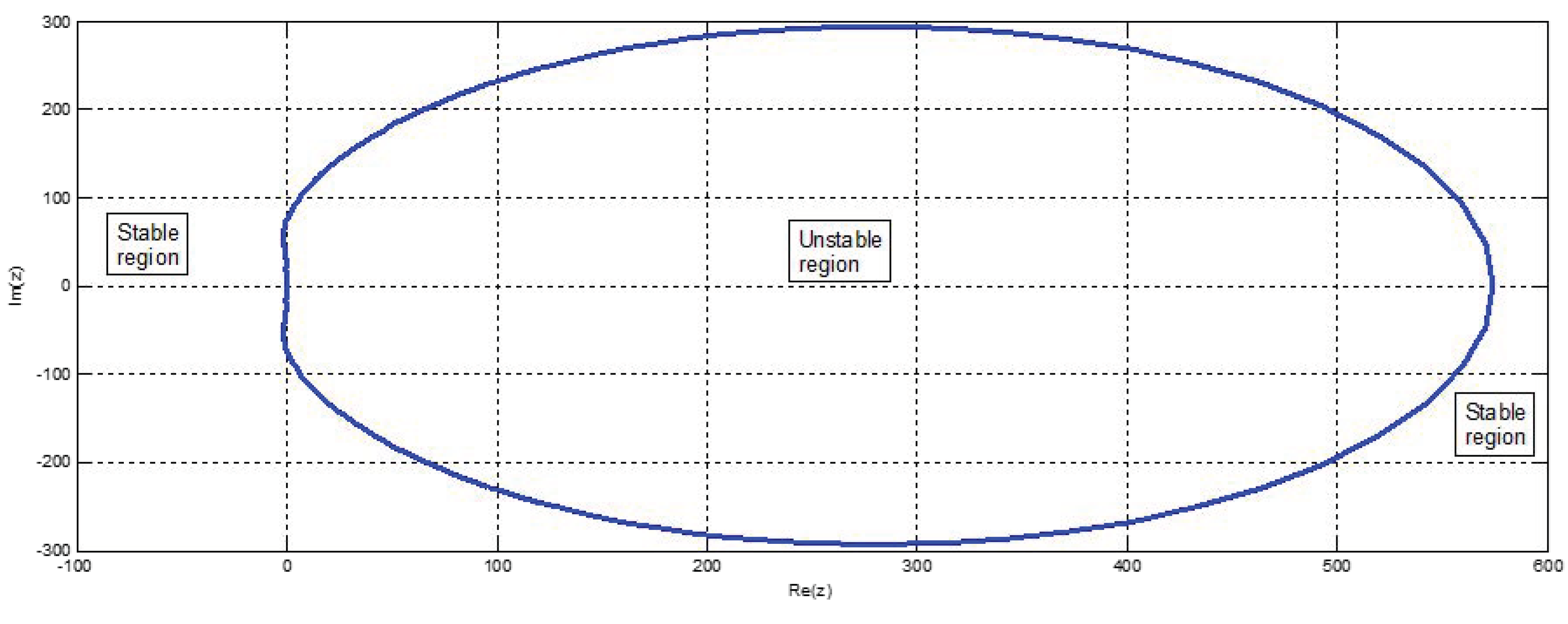
“The region of absolute stability of a numerical method is the set of complex values  $\lambda h$ for which all solutions of the test problem $y^{″}=-{\lambda }^{2}y$ will remain bounded as  $n\to \infty$”.

The boundary locus method is adopted in generating the stability polynomial of the hybrid method. The polynomial is

$$\begin{array}{l}\overline{h}(w)=-h^{14}\left(\frac{1}{195328244980512}{w}^7+\frac{383}{39065648996102404266493378560}{w}^6\right)\\ -h^{12}\left(\frac{64313}{39065648996102400}{w}^7+\frac{14662561}{117196946988307200}{w}^6\right)\\ -h^{10}\left(\frac{21601}{256261545892800}{w}^7+\frac{54664709}{1025046183571200}{w}^6\right)\\ +h^8\left(\frac{2021}{1394620657920}{w}^7-\frac{36041177}{3486551644800}{w}^6\right)-h^6\left(\frac{757}{1778852880}{w}^7+\frac{430601}{444713220}{w}^6\right)\\ -h^4\left(\frac{5077}{123480}{w}^6-\frac{23}{246960}{w}^7\right)-h^2\left(\frac{2}{147}{w}^7+\frac{94}{147}{w}^6\right)+w^7-2w^6\end{array}$$

(22)

Figure 1 shows the plot of stability region of the proposed hybrid method.

From Figure 1, it is clear the hybrid method is A–stable. The stability region is the exterior of the curve.

4. Numerical Results and Discussion

We shall simulate some second order oscillatory problems with applications to physical systems using the newly derived hybrid method.

4.1. Problem 1 (Highly Stiff Oscillatory System)

Consider the highly stiff system of oscillatory problem

$$\left[\begin{array}{l}{y}^{″}{}_1(t)\\ y^{″}{}_2(t)\end{array}\right]+\left[\begin{array}{l} 13 -12\\ -12 13\end{array}\right]\left[\begin{array}{l}{y}_1(t)\\ y_2(t)\end{array}\right]=\frac{12{\epsilon }^2}{5}\left[\begin{array}{l} 3 -2\\ -2 3\end{array}\right]\left[\begin{array}{l}{y}^{\prime }{}_1(t)\\ y^{\prime }{}_2(t)\end{array}\right]+{\epsilon }^2\left[\begin{array}{l}{f}_1(t)\\ f_2(t)\end{array}\right], \left[\begin{array}{l}{y}_1(0)\\ y_2(0)\end{array}\right]=\left[\begin{array}{l}{\epsilon }^2\\ {\epsilon }^2\end{array}\right], \left[\begin{array}{l}{y}^{\prime }{}_1(0)\\ y^{\prime }{}_2(0)\end{array}\right]=\left[\begin{array}{l}-4\\ 6\end{array}\right]$$

(23)

where $\epsilon ={10}^{-3}$, $f_1(t)=\left(36/5\right)\sin t+24\sin 5t$ and $f_2(t)=-\left(24/5\right)\sin t-36\sin 5t$. The analytical solution is given as

$$\left[\begin{array}{l}{y}_1(t)\\ y_2(t)\end{array}\right]=\left[\begin{array}{l}\sin t-\sin 5t+\epsilon \cos t\\ \sin t+\sin 5t+\epsilon \cos t\end{array}\right]$$

(24)

The results obtained in

Table 2. Comparison of global errors for Problem 1 using our method (HM) and BHM on the interval [0, 100].

$\mathit{h}$	$\mathbf{HM} {\mathit{y}}_1$	$\mathbf{BHM} {\mathit{y}}_1$	$\mathbf{HM} {\mathit{y}}_2$	$\mathbf{BHM} {\mathit{y}}_2$
$1$	2.04 × 10−2	1.57 × 10−1	2.04 × 10−2	1.57 × 10−1
$1/2$	1.21 × 10−7	9.38 × 10−5	1.21 × 10−7	9.38 × 10−5
$1/4$	1.57 × 10−9	5.29 × 10−8	1.57 × 10−9	5.29 × 10−8
$1/8$	3.14 × 10−13	1.54 × 10−11	3.14 × 10−13	1.54 × 10−11
$1/16$	6.89 × 10−17	5.07 × 10−14	6.89 × 10−17	5.07 × 10−14

clearly showed that the proposed hybrid method (which is of order eight) outperformed the block hybrid method of order eleven developed by [41]. The solution curves in Figure 2 also showed that the approximate solution obtained by the hybrid method converges to the analytical solution on the interval [0, 100]. Notice that the global error at $y_1$ and $y_2$ are same. This is because the exact solution at $y_1$ and $y_2$ are almost the same.

4.2. Problem 2 (Projectile Motion with Aerodynamic Drag)

The projectile motion (the X and Y displacements) of an object is given by the differential equations

$$m{x}^{″}+c_d{x}^{\prime }{\left({\left(x^{\prime }\right)}^2+{\left(y^{\prime }\right)}^2\right)}^{(1/2)}=0$$

(25)

$$m{y}^{″}+c_d{y}^{\prime }{\left({\left(x^{\prime }\right)}^2+{\left(y^{\prime }\right)}^2\right)}^{(1/2)}=-w$$

(26)

The differential equations were solved using the following coefficients of aerodynamic drag $c_d=\left\{0.1, 0.3, 0.5\right\} \mathrm{N}/\mathrm{m}$. Take $m=10 \mathrm{kg}$, $x^{\prime }(0)=100 {\mathrm{ms}}^{-1}$, $y^{\prime }(0)=10 {\mathrm{ms}}^{-1}$, $x(0)=0$, $y(0)=0$, $g=9.81 {\mathrm{ms}}^{-2}$ and $w=mg$, see [42].

The authors [6] simulated the problem above by converting the equations into their equivalent first order systems and then employed ode45 solver to generate their solution curves.

It is obvious from the plots in Figure 3 that as $c_d$ increases, the displacement’s maximum value decreases in the $y$ direction. In the $x$ direction, the value of the displacement for which the displacement in the $y$ direction is maximum, also decreases. The solution curves generated using the new hybrid method clearly converges to those of the curves generated by the ode45 solver at different values of the coefficients of aerodynamics $c_d$. This shows that the hybrid method is computationally reliable.

4.3. Problem 3 (Half Cylinder Rolling on a Horizontal Plane)

The governing equation for motion of a half cylinder (or semi cylinder) with mass m and radius $R$ rolling on a horizontal plane is given by the oscillatory problem,

$$\left(\frac{3m{R}^2}{2}-2mbR\sin \theta \right){\theta }^{″}-mbR\cos \theta {\left({\theta }^{\prime }\right)}^2=wb\cos \theta$$

(27)

The differential Equation (27) is solved by generating a solution curve of angle of oscillation $\theta$ against time $t$. The mass center is at $G$ located at distance $b=\frac{4R}{3\pi }\mathrm{m}$ from the cylindrical axis at $O$. Take $m=5\mathrm{kg}$,$R=0.1 \mathrm{m}$, $g=9.81 {\mathrm{ms}}^{-2}$ and $w=mg$. Figure 4 shows a typical half-cylinder on a horizontal plane with an angle of inclination $\theta$.

The authors [6] also simulated the problem above by converting the equation into its equivalent first order systems and then employed ode45 solver to generate the solution curve.

The solution curves obtained by using the new hybrid method on Problem 3 converge to those of the curves generated by the ode45 solver showing that the new hybrid method is computationally reliable, see Figure 5.

4.4. Problem 4 (The Stiefel and Bettis Oscillatory Problem)

Consider the Stiefel and Bettis oscillatory system of equations,

$$\begin{array}{l}{y}^{″}{}_1(t)+y_1(t)=0.001\cos (t), y_1(0)=1, y^{\prime }{}_1(0)=0\\ y^{″}{}_2(t)+y_2(t)=0.001\sin (t), y_2(0)=1, y^{\prime }{}_2(0)=0.9995\end{array}$$

(28)

The exact solution is given by,

$$\begin{array}{l}{y}_1(t)=0.0005t\sin (t)+\cos (t)\\ y_2(t)=-0.0005t\cos (t)+\sin (t)\end{array}$$

(29)

4.5. Problem 5 (Damped Duffing Oscillatory Problem)

Consider the damped Duffing oscillatory problem,

$$y^{″}(t)+y(t)+y^{\prime }(t)+y^2(t)y^{\prime }(t)=2\cos (t)-{\cos }^3(t), y(0)=0, y^{\prime } (0)=1$$

(30)

defined on the $0\le t\le 100$. The analytical solution is given by,

$$y(t)=\sin (t)$$

(31)

4.6. Problem 6 (Undamped Duffing Oscillatory Problem)

Consider the following undamped Duffing oscillatory problem,

$$y^{″}(t)+y(t)+y^3(t)=\xi \cos (\lambda t), y(0)={\varphi }_0, y^{\prime } (0)=0$$

(32)

where,

$$\alpha =2.00426728067\times {10}^{-1}, \xi =2.0\times {10}^{-3}, \lambda =1.01$$

(33)

The analytical solution to the problem is

$$y(t)={\displaystyle \sum _{i=0}^3{\varphi }_{2i+1}Cos\left(\left(2i+1\right)\lambda t\right)}$$

(34)

where,

$$\left\{\begin{array}{l}{\varphi }_1, {\varphi }_3,\\ {\varphi }_5, {\varphi }_7\end{array}\right\}=\left\{\begin{array}{l}2.00179477536\times {10}^{-1}, 2.4946143\times {10}^{-4}, \\ 3.04014\times {10}^{-7}, 3.74\times {10}^{-10}\end{array}\right\}$$

(35)

Table 3. Comparison of the absolute errors and execution time for Problem 4 using our method (HM) and OSHBM.

$\mathit{t}$	$\mathbf{HM} {\mathit{y}}_1$	$\mathbf{HM} {\mathit{y}}_2$	$\mathbf{OSHBM} {\mathit{y}}_1$	$\mathbf{OSHBM}{\mathit{y}}_2$	Time in HM	Time in OSHBM
0.1000	6.944134 × 10−14	2.053113 × 10−14	1.256535 × 10−12	2.826929 × 10−12	0.0321	0.4261
0.2000	7.080203 × 10−14	2.759703 × 10−14	2.113954 × 10−12	5.899430 × 10−12	0.0493	0.4362
0.3000	7.764101 × 10−14	5.796163 × 10−14	2.376410 × 10−12	6.830921 × 10−12	0.0667	0.4621
0.4000	7.888446 × 10−14	6.826273 × 10−14	3.424150 × 10−12	1.499123 × 10−12	0.1056	0.4891
0.5000	7.810730 × 10−14	6.264544 × 10−14	3.394396 × 10−12	1.839452 × 10−12	0.1229	0.5001
0.6000	7.678613 × 10−14	6.505462 × 10−14	3.343548 × 10−12	1.655884 × 10−11	0.1419	0.5201
0.7000	7.554268 × 10−14	6.540990 × 10−14	4.294920 × 10−12	1.247034 × 10−11	0.1594	0.5578
0.8000	7.457679 × 10−14	8.378897 × 10−14	4.257394 × 10−12	8.431255 × 10−11	0.1768	0.5881
0.9000	7.397727 × 10−14	8.072475 × 10−14	5.234413 × 10−12	5.323966 × 10−11	0.1939	0.6101
1.0000	7.377743 × 10−14	8.038814 × 10−14	6.226530 × 10−12	3.212587 × 10−11	0.2885	0.6312

,

Table 4. Comparison of the number of steps, maximum error and average errors for Problem 5 using our method (HM) and VOVSM.

TOL	Method	Steps	MAXERR	AVERR
${10}^{-2}$	HM	209	2.12651 × 10−5	4.81903 × 10−6
	VOVSM	217	1.07600 × 10−1	3.03894 × 10−2
${10}^{-4}$	HM	264	3.19061 × 10−7	1.41210 × 10−8
	VOVSM	284	1.24649 × 10−3	1.92899 × 10−4
${10}^{-6}$	HM	316	1.29139 × 10−9	1.09310 × 10−9
	VOVSM	330	1.28039 × 10−5	3.26641 × 10−6
${10}^{-8}$	HM	486	4.90431 × 10−10	7.19038 × 10−10
	VOVSM	499	7.27324 × 10−7	1.46368 × 10−7
${10}^{-10}$	HM	740	4.34750 × 10−13	4.12474 × 10−13
	VOVSM	772	7.83863 × 10−9	2.03721 × 10−9

and

Table 5. Comparison of the end-point absolute errors and execution time for Problem 6 using our method (HM) and OSHBM.

$h$	ABSERR	ABSERR	Time	Time
	in HM	in OSHBM	in HM	in OSHBM
$m/500$	6.000145 × 10−17	2.256151 × 10−16	1.2676	2.0032
$m/1000$	4.010991 × 10−17	1.678127 × 10−16	1.6272	2.2001
$m/2000$	2.102903 × 10−17	6.061690 × 10−17	2.1287	3.1245
$m/3000$	1.211451 × 10−17	5.167032 × 10−17	2.2781	3.6234
$m/4000$	3.190380 × 10−18	4.267817 × 10−17	3.0182	4.0151
$m/5000$	2.201181 × 10−18	2.762717 × 10−17	4.0167	6.1930

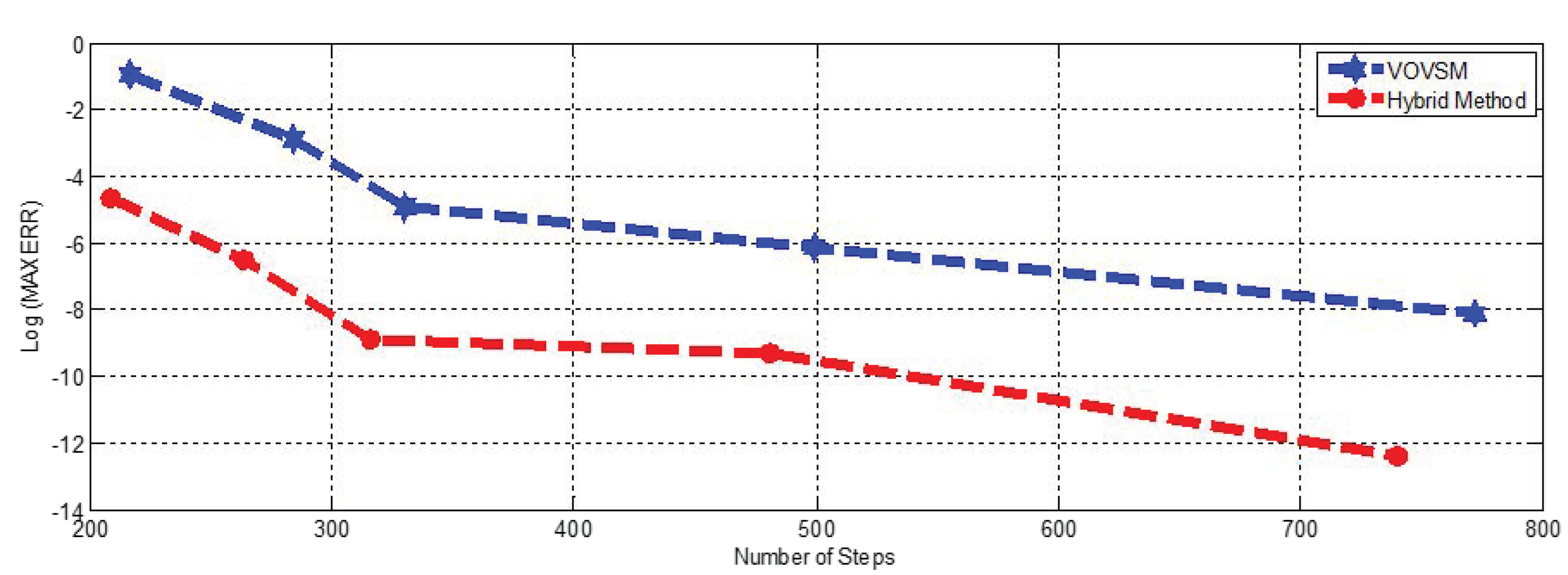
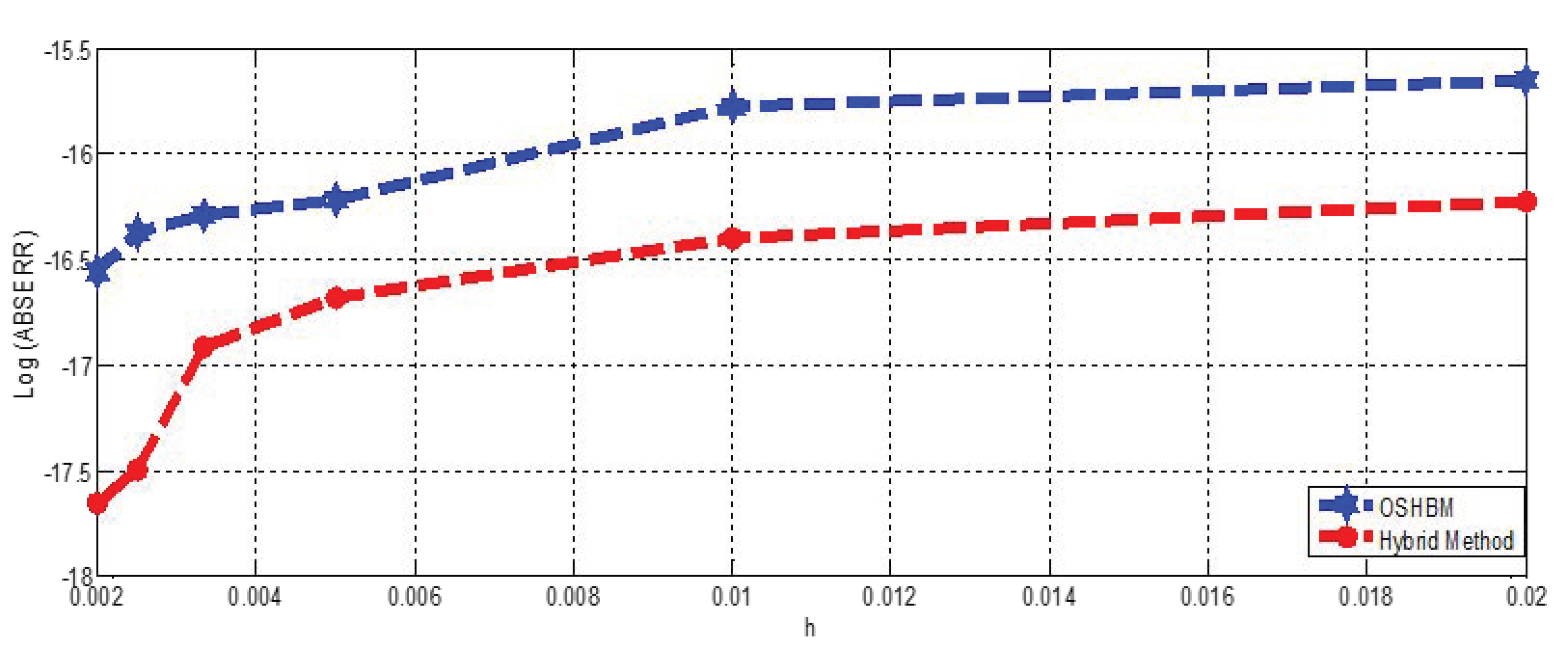
Note that $m=10$ in Table 5.

display the performance of the new hybrid method on Problems 4–6 in comparison to other existing methods. The numerical results clearly showed that the new hybrid method performed better than the methods we juxtaposed our results with in terms of the number of steps taken, absolute errors, maximum errors, average errors and computation time. In Figure 5 for instance, it is obvious that the approximate solution obtained using the hybrid method agree with the solution obtained using ode45 solver for Problem 3. For Problem 4, it is clear that the approximate solution using the hybrid method converges to the exact solution, see Figure 6. Thus, the new hybrid method outperformed the methods we juxtaposed our results with. The execution time (in seconds) further showed that the new hybrid method is more efficient in terms of the economy of computer time (and also more accurate than the OSHBM developed by [38]) for Problems 4 and 6, see Table 3 and Table 5 respectively. Table 4 also shows that the hybrid method is more accurate than the VOVSM developed by [38] in terms of maximum and average errors. Also, the hybrid method requires fewer numbers of steps than the VOVSM. Figure 7 and Figure 8 further buttress the fact that the hybrid method is more accurate for Problems 5 and 6.

4.7. Problem 7 (The Van der Pol Model)

The Van der Pol equation, a nonlinear stiff equation is given by,

$$y^{″}(t)+\mu \left(1+y^2(t)\right)y^{\prime }(t)+y(t)=0$$

(36)

This nonlinear model does not have a closed form solution, thus, we need to obtain an approximate solution using the new hybrid method. Firstly, Equation (36) is transformed to an equivalent system of equations of the form

$$\left.\begin{array}{l}{y}_1^{\prime }(t)=y_2(t), y_1(0)=2\\ y_2^{\prime }(t)=\left[-y_1(t)+(1-y_1^2(t))y_2(t)\right]/\in , y_2(0)=0\end{array}\right\}$$

(37)

defined on the interval [0, 70]. This transformation is achieved by substituting $y_1(t)=\phi (t), y_2(t)=\mu {\phi }^{\prime }(t)$ and $t=t/\mu$, where $\in =1/{\mu }^2$ is a parameter that controls stiffness. In this paper, we assume $\in =500$.

Since the Van der Pol model does not have a closed form solution, the approximate solution using the new hybrid method was compared with those of FPHBI developed by [36] and ode 15s at the end points $x=1$, $x=5$, $x=10$ and $x=20$. The numerical solution and accuracy curves generated clearly showed that the new hybrid method is accurate and computationally reliable, see

Table 6. Comparison of approximate solutions for Problem 7 at $h=0.1$.

$\mathit{t}$	${\mathit{y}}_{\mathit{i}}$	APPSOL (HM)	APPSOL (FPHBI)	APPSOL (ode 15s)
$1$	$y_1$	$-1.8650951120$	$-1.8650950931$	$-1.8650950571$
	$y_2$	$0.7524845401$	$0.7524845342$	$0.7524845299$
$5$	$y_1$	$1.8985234609$	$1.8985234584$	$1.8985234421$
	$y_2$	$-0.7289532599$	$-0.7289532571$	$-0.7289532451$
$10$	$y_1$	$1.7865365312$	$1.7865365214$	$1.7865365103$
	$y_2$	$-0.8156276678$	$-0.8156276595$	$-0.8156276438$
$20$	$y_1$	$1.5075643427$	$1.5075643297$	$1.5075643177$
	$y_2$	$-1.1911230055$	$-1.1911230041$	$-1.1911230003$

and Figure 9 respectively.

It is therefore obvious that the proposed hybrid method is accurate and efficient. The research works earlier carried out by [46,47,48,49,50,51,52] on the derivations, implementations and applications of numerical methods on physical systems may also be consulted for more details.

5. Conclusions

In this research, a hybrid method was formulated for the simulations of second order oscillatory problems with applications to physical systems. The results clearly showed that the new method is efficient, accurate and reliable. The properties of the method were also analyzed and it is obvious that the method is zero-stable, consistent and convergent. The region of absolute stability of the method also showed that the method is A-stable, thus, making it suitable for the solutions and simulations of problems of the form (1). In view of the foregoing, the proposed hybrid method is therefore recommended for the simulations and solutions of physical systems of second order. Further research may also extend this work, by considering the possibility of proposing new methods for simulating larger systems of equations.

References

Musaev, H.K. The Cauchy problem for degenerate parabolic convolution equation. TWMS J. Pure Appl. Math.2021, 12, 278–288. [Google Scholar]
Wend, D.V.V. Uniqueness of solution of ordinary differential equations. Am. Math. Mon.1967, 74, 27–33. [Google Scholar] [CrossRef]
Raisinghania, M.D. Ordinary and Partial Differential Equations; S. Revised edition; Chand and Company LTD: New-Delhi, India, 2014. [Google Scholar]
Abolfazl, J.; Hadi, F. The application of Duffing oscillator in weak signal detection. ECTI Trans. Electr. Eng. Electron. Commun.2011, 9, 1–6. [Google Scholar]
Soraya, H. Pendulum with aerodynamic and viscous damping. J. Appl. Inf. Commun. Technol.2016, 3, 43–47. [Google Scholar] [CrossRef]
Harihara, P.; Childs, D.N. Solving Problems in Dynamics and Vibration Using MATLAB; Department of Mechanical Engineering, Texas A and M University College Station: College Station, TX, USA, 2020; pp. 1–104. [Google Scholar]
Zhang, W.B. Differential Equations, Bifurcations, and Chaos in Economics; World Scientific Publishing: Hackensack, NJ, USA, 2005. [Google Scholar]
Sunday, J.; Chigozie, C.; Omole, E.O.; Gwong, J.B. A pair of three-step hybrid block methods for the solutions of linear and nonlinear first-order systems. Util. Math.2021, 118, 1–15. [Google Scholar] [CrossRef]
Adiguzel, R.S.; Aksoy, U.; Karapinar, E.; Erthan, I.M. On the solutions of fractional differential equations via Geraghty type hybrid contractions. Appl. Comput. Math.2021, 20, 313–333. [Google Scholar]
Aliev, F.A.; Aliyev, N.A.; Hajiyeva, N.S.; Mahmudov, N.I. Some mathematical problems and their solutions for the oscillating systems with liquid dampers: A review. Appl. Comput. Math.2021, 20, 339–365. [Google Scholar]
Shokri, A.; Tahmourasi, M. A new two-step Obrechkoff method with vanished phase-lag and some of its derivatives for the numerical solution of radial Schrödinger equation and related IVPs with oscillating solutions. Iran. J. Math. Chem.2017, 8, 137–159. [Google Scholar]
Marian, D.; Ciplea, S.A.; Lungu, N. Ulam-Hyers stability of Darboux-Lonescu problem. Carpathian J. Math.2021, 37, 211–216. [Google Scholar] [CrossRef]
Adeyefa, E.O.; Omole, E.O.; Shokri, A. Numerical solution of second-order nonlinear partial differential equations originating from physical phenomena using Hermite based block methods. Results Phys.2023, 46, 106270. [Google Scholar] [CrossRef]
Noor, M.A.; Noor, K.I. Some new classes of strongly generalized preinvex functions. TWMS J. Pure Appl. Math.2021, 12, 181–192. [Google Scholar]
Akbarov, S.D.; Mehdiyev, M.A.; Zeynalov, A.M. Dynamic of the moving ring-load acting in the interior of the bi-layered hollow cylinder with imperfect contact between the layers. TWMS J. Pure Appl. Math.2021, 12, 223–242. [Google Scholar]
Tongxing, L.; Yuriy, V.R.; Shuhong, T. Oscillation of second-order nonlinear differential equations with damping. Math. Slovaca2014, 64, 1227–1236. [Google Scholar]
Juraev, D.A. On the Cauchy problem for matrix factorizations of the Helmholtz equation in an unbounded domain in R2. Sib. Electron. Math. Rep.2018, 15, 1865–1877. [Google Scholar]
Marian, D.; Ciplea, S.A.; Lungu, N. Ulam-Hyers stability of Euler’s equation in the calculus of variations. Mathematics2021, 9, 3320. [Google Scholar] [CrossRef]
Juraev, D.A. The Cauchy problem for matrix factorization of the Helmholtz equation in an unbounded domain. Sib. Electron. Math. Rep.2017, 14, 752–764. [Google Scholar]
Larin, V.B.; Tunik, A.A. Two-stage procedure of H∞-parameterization of stabilizing controllers applied to quadrotor flight control. TWMS J. Pure Appl. Math.2021, 12, 199–208. [Google Scholar]
Davvaz, B.; Mohammadi, F. Different types of ideals and homomorphisms of (m, n)-semirings. TWMS J. Pure Appl. Math.2021, 12, 209–222. [Google Scholar]
Pankov, P.S.; Zheentaeva, Z.K.; Shirinov, T. Asymptotic reduction of solution space dimension for dynamical systems. TWMS J. Pure Appl. Math.2021, 12, 243–253. [Google Scholar]
Chen, W.; Wu, W.X.; Teng, Z.D. Complete dynamics in a nonlocal dispersal two-strain SIV epidemic model with vaccination and latent delays. Appl. Comput. Math.2020, 19, 360–391. [Google Scholar]
Yusufoglu, E. Numerical solution of Duffing equation by the Laplace decomposition algorithm. Appl. Math. Comput.2006, 177, 572–580. [Google Scholar]
Iskandarov, S.; Komartsova, E. On the influence of integral perturbations on the boundedness of solutions of a fourth-order linear differential equation. TWMS J. Pure Appl. Math.2022, 13, 3–9. [Google Scholar]
Hamidov, S.I. Optimal trajectories in reproduction models of economic dynamics. TWMS J. Pure Appl. Math.2022, 13, 16–24. [Google Scholar]
Nourazar, S.; Mirzabeigy, A. Approximate solution for nonlinear Duffing oscillator with damping effect using the modified differential transform method. Sci. Iran. B2013, 20, 364–368. [Google Scholar]
Kalsoom, H.U.; Ali, M.A.; Abbas, M.U.; Budak, H.Ü.; Murtaza, G.H. Generalized quantum Montgomery identity and Ostrowski type inequalities for preinvex functions. TWMS J. Pure Appl. Math.2022, 13, 72–90. [Google Scholar]
He, J.H. Variational iteration method. A kind of nonlinear analytical technique. Int. J. Nonlinear Mech.1999, 34, 699–708. [Google Scholar] [CrossRef]
Obarhua, F.O.; Kayode, S.J. Continuous explicit hybrid method for solving second order ordinary differential equations. Pure Appl. Math. J.2020, 9, 26–31. [Google Scholar] [CrossRef]
Rasedee, A.F.N.; Ishak, N.; Hamzah, S.T.; Ijam, H.M.; Suleiman, M.; Ibrahim, Z.B.; Sathar, M.H.A.; Ramli, N.A.; Kamaruddin, N.S. Variable order variable step-size algorithm for solving nonlinear Duffing oscillator. J. Phys. Conf. Ser.2017, 890, 012045. [Google Scholar] [CrossRef] [Green Version]
Sunday, J.; Kumleng, G.M.; Kamoh, N.M.; Kwanamu, J.A.; Skwame, Y.; Sarjiyus, O. Implicit four-point hybrid block integrator for the simulations of stiff models. J. Niger. Soc. Phys. Sci.2022, 4, 287–296. [Google Scholar] [CrossRef]
Khashan, M.M.; Syam, M.I.; Alomari, A.K. Numerical solution of cubic free undamped Duffing oscillator equation using continuous implicit hybrid method. Ital. J. Pure Appl. Math.2019, 42, 588–597. [Google Scholar]
Kwari, L.J.; Sunday, J.; Ndam, J.N.; James, A.A. On the numerical approximation and simulation of damped and undamped Duffing oscillators. Sci. Forum J. Pure Appl. Sci.2021, 21, 503–515. [Google Scholar] [CrossRef]
Yakubu, S.D.; Yahaya, Y.A.; Lawal, K.O. Three-step block hybrid linear multistep method for solution of special second order ordinary differential equations. J. Niger. Math. Soc.2021, 40, 149–160. [Google Scholar]
Awari, Y.S. Some generalized two-step block hybrid Numerov method for solving general second order ordinary differentialequations without predictors. Sci. World J.2015, 12, 12–18. [Google Scholar]
Jator, S.N.; King, K.L. Integrating oscillatory general second-order initial value problems using a block hybrid method of order 11. Math. Probl. Eng.2018, 2018, 3750274. [Google Scholar] [CrossRef]
Sunday, J.; Ndam, J.N.; Kwari, L.J. An accuracy-preserving block hybrid algorithm for the integration of second-order physical systems with oscillatory solutions. J. Niger. Soc. Phys. Sci.2023, 5, 1017. [Google Scholar] [CrossRef]
Lambert, J.D. Numerical Methods for Ordinary Differential Systems: The Initial Value Problem; John Wiley and Sons Ltd.: Hoboken, NJ, USA, 1991. [Google Scholar]
Lambert, J.D. Computational Methods in Ordinary Differential Equations; John Wiley & Sons, Inc.: New York, NY, USA, 1973. [Google Scholar]
Fatunla, S.O. Numerical integrators for stiff and highly oscillatory differential equations. Math. Comput.1980, 34, 373–390. [Google Scholar] [CrossRef]
Dahlquist, G.G. Convergence and stability in the numerical integration of ordinary differential equations. Math. Scand.1956, 4, 33–50. [Google Scholar] [CrossRef] [Green Version]
Shokri, A.; Mehdizadeh Khalsaraei, M.; Molayi, M. Nonstandard dynamically consistent numerical methods for MSEIR model. J. Appl. Comput. Mech.2022, 8, 196–205. [Google Scholar]
Sunday, J.; Shokri, A.; Akinola, R.O.; Joshua, K.V.; Nonlaopon, K. A convergence-preserving non-standard finite difference scheme for the solutions of singular Lane-Emden equations. Results Phys.2022, 42, 106031. [Google Scholar] [CrossRef]
Rufai, M.A.; Shokri, A.; Omole, E.O. A one-point third-derivative hybrid technique for solving second-order oscillatory and periodic problems. J. Math.2023, 2023, 2343215. [Google Scholar] [CrossRef]
Kuboye, J.O.; Omar, Z. Derivation of a six-step block method for direct solution of second order ordinary differential equations. Math. Comput. Appl.2015, 20, 151–159. [Google Scholar]
Sunday, J.; Shokri, A.; Kwanamu, J.A.; Nonlaopon, K. Numerical integration of stiff differential systems using non-fixed step-size strategy. Symmetry2022, 14, 1575. [Google Scholar] [CrossRef]
Argyros, I.K.; Santhosh, G. Extended Kung-Traub-type method for solving equations. TWMS J. Pure Appl. Math.2021, 12, 193–198. [Google Scholar]
Figure 1.
Region of absolute stability of the hybrid method.
Figure 2.
Solution curves for Problem 1 on the interval [0, 100].
Figure 3.
Solution curves for Problem 2 showing the and displacements on the interval [0, 100].
Figure 4.
Schema of a half cylinder rolling on a horizontal plane.
Figure 5.
Solution Curves for Problem 3 showing the angle of inclination against time.
Figure 6.
Solution curves for Problem 4 on the interval [0, 80].
Figure 7.
Accuracy curves for Problem 5.
Figure 8.
Accuracy curves for Problem 6.
Figure 9.
Solution curves for Problem 7 on the interval [0, 70].