A Supply Chain Model with Learning Effect and Credit Financing Policy for Imperfect Quality Items under Fuzzy Environment

Abstract

In this paper, the seller offers a credit period to his buyer for more sales and the buyer accepts the seller’s policy to gain more profit, and it is assumed that the seller has defective and non-defective items. When the seller provides lots for sale to his buyer then, the buyer separates the whole lots with the help of inspection process into defective and perfect quality items. Further, in this scenario, the percentage of defective items present in the lot follows the S-shape learning curve and it is also considered that the demand rate is imprecise in nature. Here, the demand rate assumes a triangular fuzzy number due to the imprecise nature and it is the model assumption. Based on this assumption, we developed an inventory model with the effect of learning and trade credit strategy under a fuzzy environment for the buyer. The buyer’s total profit has been optimized concerning the order quantity in the fuzzy environment where order quantity has been assumed as a decision variable. The results of this model were verified with the help of numerical examples and sensitivity analysis. We compared the buyer’s total profit in a crisp and fuzzy environment and the buyer gained more profit in a fuzzy environment compared to the crisp environment. Moreover, we compared the results with and without the effect of learning and trade credit on the buyer’s ordering policy and obtained a positive effect on the ordering policy in the numerical section. We determined positive results from the sensitivity analysis, which proved that the trade credit policy will be beneficial for both partners of the supply chain.

1. Introduction

In most of the models, it is always seen that all the products are of perfect nature. However, in the real scenario, it is not so. The companies’ inspection policies can uphold their reputation as well as fulfill customer demand and maximize their profit. In our modern business world, one of the most effective tools in the inventory system is trade credit. Trade credit benefits buyers by permitting them to buy merchandise via bank account transfer and not paying cash quickly, or maybe paying the provider at aa later planned date. Trade credit is the most popular financing method adopted by manufacturers, retailers, vendors, and buyers to accelerate the sale of their product. The knowledge of the comfort of paying in part benefits the buyer compared to paying the full amount right away. Human performance shows enhancement when activities are undertaken in regular and repetitive manner. The time required to implement a task decreases with increasing repetition. This led to the birth of the concept—learning theory. By learning effect, we could estimate optimal time, cost for production with optimal decisions for prices, as well as reduce labor hours. The performance of the learning curve with mathematical pictures has been presented by Wright [1]. After that, Li and Chang [2], Jaber and Bonney [3] and Jaber and Bonney [4] discussed the impact of learning in many aspects with Wright [1], and applied it to both financial order quantity and economic production quantity problems in order to analyze the effect of learning on the most sensitive decision, i.e., batch length for quantity of irregular production runs. In reality, it has been seen that some uncertainty or randomness occurs in every real-life problem. To handle these hesitations mathematically, fuzzy set theory should be more reliable and easier to apply.

To sum up in brief, this paper focuses on:

• Inventory model with imperfect items;
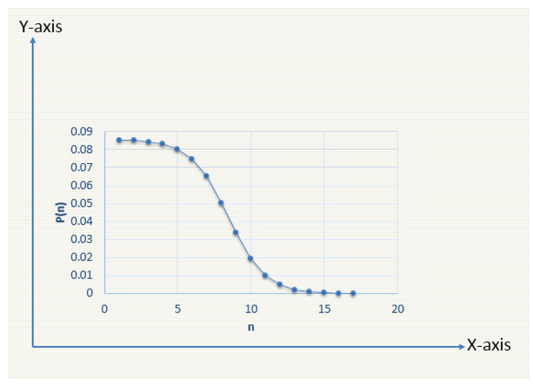
• Portion of defective items following learning curve and its effect on order quantity and buyer’s profit;
• Credit financing strategy considerations and their impact on the lots and buyer’s profit;
• Demand represented as triangular fuzzy number;
• Role of fuzzy environment.

2. Literature Review

Inventory management has a vast research history dating back to the middle of the twentieth century, where several researchers have exerted great effort into formulating realistic models for the inventory. Many distinguished researchers who worked on inventory control and management, such as Shah [5], Shah [6], Aggarwal and Jaggi, [7] and Hwang and Shinn [8], extended Goyal [9] inventory model with the reflection of a constant decaying rate. To accommodate allowances for shortages, Jamal et al. [10] modified the model of Aggarwal and Jaggi [7]. In Kim et al. [11], seller’s profit cap was maximized by the invented maximized time period of financing period for the items. In Chung [12], a model was established with a discount payment flow towards the logical examination of the finest stock plan in the policy of trade credit. Then, in Shah and Shah [13], a model was formed with a probabilistic stock model under payment’s delay policy. After that, Chu et al. [14] and Jamal et al. [15] worked on the determination of the optimal time period for payments. In Chang et al. [16], a quantity model was discovered for deteriorating items where the time period of late is directly associated with the lot size. For calculating the optimized prices for the retailers in Shinn and Hwang [17], a mathematical model was developed. The model by Huang and Chung [18] upgraded Goyal [9] model with the renewal of cash policy and its aim to reduce the annual buyer’s inventory cost with trade credit from the seller’s insight. In the current periods, many inventory models with two-level credit financing approach are developed. In Teng et al. [19], a formula for production was formulated, where the manufacturer obtains a credit period from the dealer’s end and provides supporting time period to customers. Jaggi, et al. [20] enriched a model with the help of two-level credit policy under credit linked with the demand function. In this continuation from Chen and Kang [21], a two-level trade credit inventory model with a negotiation scheme under the amount sensitive demand was formulated. In Jaggi et al. [22], a mathematical model for the inventory was proposed for the imperfect items with the policy of financing period under shortages. In Jaber and Salameh [23], a mathematical model was derived with shortages and backorder under leaning effect. Then, in Jaber and Bonney [24], a construction model was offered with the help of learning models such as LFCM, VRIF and VRVF and compared the obtained results to determine the model flexibility. Further, in Jaber et al. [25], the idea was stretched with the help of learning concepts for the imperfect items. A mathematical idea under impact of learning for the imperfect items was established in Khan et al. [26]. In Jaber and Khan [27], a model was discussed about the order of lots and the number of shipments for the imperfect items using the concept of learning. An inventory model with different kinds of learning curves and a comparison were created in Anzanello and Fogliatto [28]. In Wee et al. [29], a mathematical inventory model was improved under shortages. Then, in Lin et al. [30], a supplier–retailer inventory model was investigated with imperfect items under the financing period strategy. A model for defective items under learning effect and shortages was offered by Konstantaras et al. [31]. After that, in Shah et al. [32], formulations were represented with delay in payments and the fuzzy total cost function was defuzzified by the center of gravity rule. An optimal policy for the production model under learning and trade credit scenario were proposed by Teng et al. [33]. The model by Jaggi et al. [34] analyzed the deterioration influence on stocks model for products with defective quality products. In Sarkar [35], the author focused on fixed life time products based on supply chain models with inspection, discount policy and also variable backorder considerations. In Sangal et al. [36], a crisp and fuzzy inventory models were formed for non-instantaneous decaying things. An order quantity model with learning effect employing shortages under the fuzzy environment was suggested in Agarwal et al. [37]. In Jaggi et al. [38], a two-storage facility system with price dependent demand for decaying products under the strategy of financing system was explained. An inventory mathematical model by Nobil et al. [39] was developed under a cleaner production environment.

In Patro et al. [40], a fuzzy inventory model was investigated for decaying and imperfect items with learning effect. An EOQ with carbon release scenario for deteriorating and defective feature items was suggested in Tiwari et al. [41]. In Jayaswal et al. [42], a learning concept was considered for defective items with the policy of credit financing, optimized order quantity and the retailer’s profit. Then, in Jayaswal et al. [43], a model was formed for defective quality items under the financing period strategy with the considerations of the impact of learning. After that, an optimal quantity model of Sangal et al. [44] was proposed with learning impact and shortages where deterioration is a function of time. In De and Mahata [45], an inventory model was investigated for defective items under cloudy fuzzy atmosphere. The commendable work in De and Mahata [45] has been improved by this present paper with the help of a learning effect and the financing period, where defective items follow the S-shape learning curve. Further, Mittal and Sharma [46] proposed a supply chain model with growing defective items under credit policy. Jayaswal et al. [47] presented an ordering policy model with the effect of learning for deteriorating defective items under the credit policy scheme. Pattnaik [48] explained a defective item-based inventory model for EOQ under fuzzy environment where demand is a function of selling price. Rajeswari et al. [49] developed an inventory model for EOQ under fuzzy environment. Mahapatra et al. [50] described a preservation-based inventory model with time-dependent deteriorating rate under fuzzy learning theory. Taheri and Mirzazadeh [51] generalized a mathematical model for the defective items under fuzzy system. Dinagar and Manvizhi [52] proposed a single-stage fuzzy-based inventory model under shortages and reworked process for defective items. Garg et al. [53] assumed an inventory model with scrap for defective items under fuzzy environment. Kuppulakshmi et al. [54] considered a fuzzy-based inventory model for defective items under penalty cost. The effects of learning operate as a significant function for reducing the inventory cost and also optimizing the total profit of the inventory system. Some authors discussed the results of the learning shape in the same direction, such as Wright [1] and Jaber et al. [25]. From Figure 1, it can be observed that the curve rises slowly as one becomes familiar with the basics of a skill. The steep part occurs when one has enough experience to start “putting it all together.’’ Then, a second phase of fast development is entered, known as Learning Phase 2. Skills are added along with the progress. At a certain moment, development achieves a speed of steady development, followed by a period of slower development. The final phase of top of the progress is known as maturity phase.

In Figure 2, the S-shape learning curve is graphically represented with the help of the available data which is provided below in the form of a formula: $P\left(n\right)=\frac{a}{g+e^{bn}},\hspace{0.17em}a>0,g>0,$ where $b$ represents the parameter of learning and $n$ is the shipment.

The present study assumes that when each article undergoes the inspection process, the demand rate should be less than or equal to the screening rate, otherwise cases of shortages may occur, and at the same time, this consideration also affects the demand completion of perfect quality items. Further, the faulty items are traded immediately as a single lot at a reduced price. The portion of imperfect quality items behaves in the S-shaped learning curve. By the application of the fuzzy method, problems regarding the imprecise nature of demand rate in the corporate world have been reduced here. In this regard, the current article examines the influence of a buyer’s optimal decisions for defective items under inspection and credit financing where the demand rate is imprecise in nature. The numerical example reveals that this proposed model with suitable defuzzification methods provides maximum retailer’s profit. Conclusively, the validity of the present model sensitive analysis has been presented and the contribution of the present paper has been shown at the bottom of the

Table 1. Author contributions.

Author(s)	Learning Approach	Screening Concept	Trade Credit Period	Defective Items	Fuzzy Environment
Wright [1]	✔
Li and Cheng [2]	✔
Jaber et al. [3,4]	✔	✔		✔
Aggrawal and Jaggi [7]		✔		✔
Salameh and Jaber [7]		✔		✔
Kim et al. [11]			✔
Shin et al. [17]		✔	✔
Jaggi et al. [22]		✔	✔	✔
Jaber et al. [25]	✔	✔		✔
Khan et al. [26]	✔	✔		✔
Anazanello et al. [28]	✔
Jaggi et al. [34]				✔
Sarkar et al. [35]		✔
Sangal et al. [36]	✔
Jaggi et al. [38]		✔	✔	✔
Tiwari et al. [41]		✔	✔	✔
Jayaswal et al. [42]	✔	✔	✔	✔
Patro et al. [40]	✔	✔
De and Mahata [45]		✔		✔	✔
Alsaed et al. [55]	✔			✔	✔
Present Paper	✔	✔	✔	✔	✔

.

3. Preliminary Definition

There are some definitions which need to be discussed for the model proposed below and, as suggested by De and Mahata [45] and Björk [56] with the consideration of the fuzzy environment in the mathematical model, the following definitions are mentioned below for more clarity.

Definition 1.

Suppose that the universal set is $X$ and any set $Y$ is defined on $X$ , then fuzzy set of $Y$ on $X$ is shown by $\widetilde{ Y}$ , then the fuzzy set can be written as $\widetilde{ Y}=\left\{\left(r, {\lambda }_{\tilde{Y}}\left(\tilde{r}\right)\right):r\in X\right\}$ where ${\lambda }_{\widetilde{ Y}}$ is the membership function and it is defined as ${\lambda }_{\widetilde{ Y}}:X\to \left[0,1\right]$ . It is considered that $\left(s_1,s_2,s_3\right)$ is a triplet with the condition $s_1<s_2<s_3$ and treated as triangular fuzzy number. The continuous membership function can be defined as

$${\lambda }_{\widetilde{ W}}=\{\begin{array}{c}\frac{s-s_1}{s_2-s_1} s_1\le s\le s_2\\ \frac{s_3-s}{s_3-s_2} s_2\le s\le s_3\\ 0 Otherwise\end{array}.$$

Definition 2.

Suppose that $p$ is any real number and$0\in X$ , then the signed distance from$p$ to$0$ can be defined by$d\left(p,0\right)=p$ and when$p<0,$ the signed distance from$c$ to$0$ is$d\left(-p,0\right)=-p.$ Assume that Ω is the family of fuzzy sets$\tilde{B}$ defined on$X$ , then$\alpha -cut,C\left(\alpha \right)=\left[B_L\left(\alpha \right),B_U\left(\alpha \right)\right]$ exists;$\forall \alpha ϵ\left[0,1\right]$ ,$B_L\left(\alpha \right)$ and$B_U\left(\alpha \right)$ is the continuous function on$\alpha$ . Then, we can write the value of$B\left(\alpha \right)$ which is$B\left(\alpha \right)={{\displaystyle \mathrm{U}}}_{0\ll \alpha \ll 1}\left[B_L{\left(\alpha \right)}_{\alpha }, B_U{\left(\alpha \right)}_{\alpha }\right]$. Then, the signed distance formula from$\tilde{B}$ to$\tilde{0}$ as written by Björk [56] is given below:

$$d\left(\tilde{B},\tilde{0}\right)=\frac{1}{2}{\displaystyle {\int }_0^1\left({\tilde{B}}_L\left(\alpha \right)+{\tilde{B}}_R\left(\alpha \right)\right)}\hspace{0.17em}d\alpha ,$$

(1)

where $\tilde{B}\in \Omega$ represents the family of fuzzy sets. If the triangular fuzzy number is $\widetilde{ A}=\left(x_1,x_2,x_3\right)$ , then $\alpha$ -cut of $\widetilde{ A}$ is $A\left(\alpha \right)=\left[A_L\left(\alpha \right),A_U\left(\alpha \right)\right]$ for $\alpha \in \left[0, 1\right],$ where $A_L\left(\alpha \right)=x_1+\left(x_2-x_3\right)\alpha$ and $A_U\left(\alpha \right)=x_3-\left(x_3-x_2\right)\alpha$ . The formula of signed distance from $\tilde{A}$ to $\tilde{0}$ is

$$d\left(\tilde{A},\hspace{0.17em}\tilde{0}\right)=\frac{\left(x_1+2x_2+x_3\right)}{4}.$$

(2)

4. Assumptions

The following are the assumptions:

• The continuity of replacement is allowed.
• Lead time and shortages are not involved in this model.
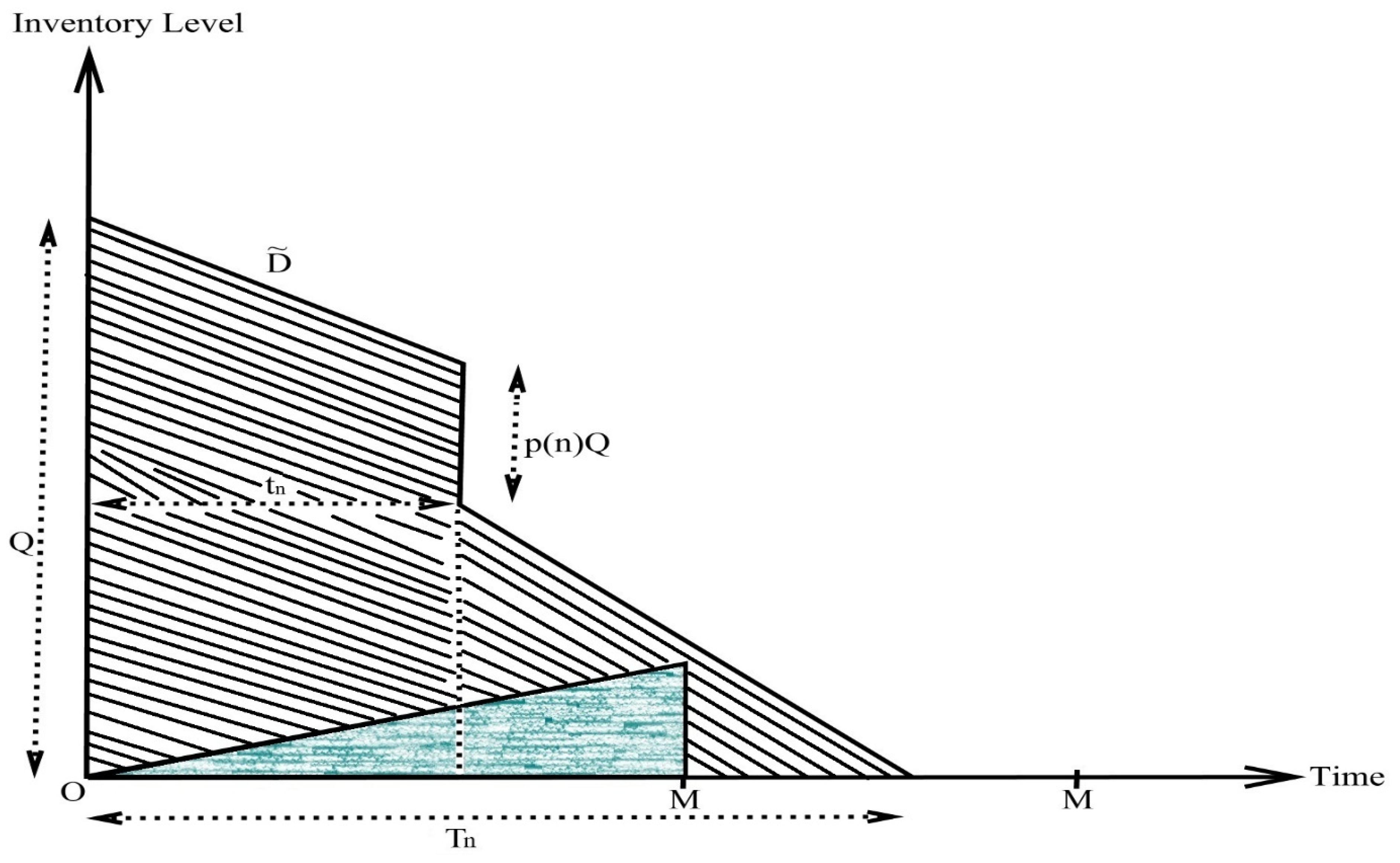
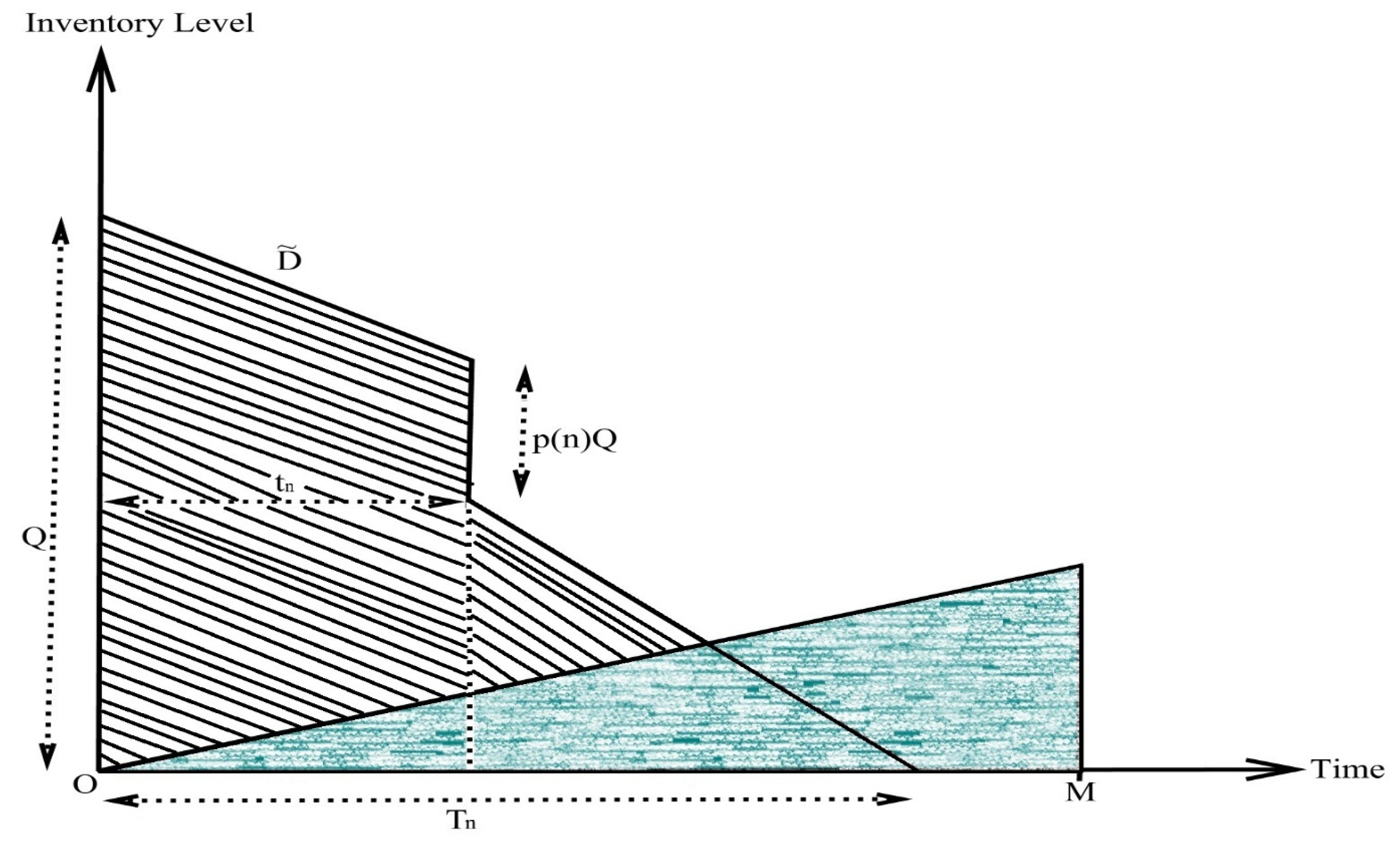
• The credit financing policy is allowed, according to Jaggi et al. [22].
• The inspection rate is greater than the demand rate, according to Jaggi et al. [22].
• Time horizon is considered to be definite.
• Demand rate is assumed imprecise in nature and taken in the form of a triangular fuzzy number in this model, according to Björk [56].
• The imperfect quality item is present in the lots delivered by the seller using the concept of Salameh and Jaber [57].
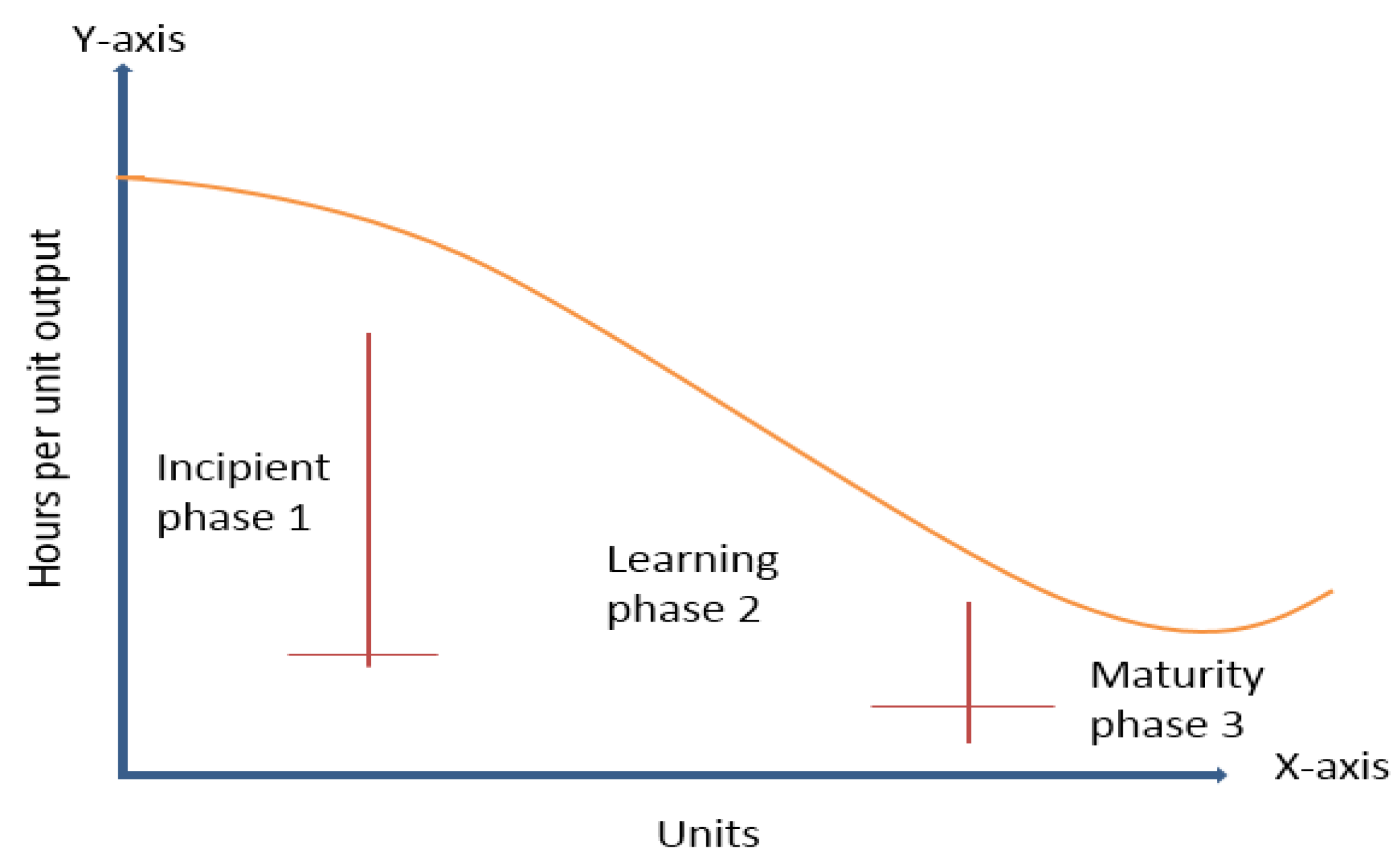
• Imperfect quality items follow the S-shape learning curve as suggested by Jaber et al. [25].
• Defective items are sold at a rebate discount.

5. Mathematical Model under Crisp Environment

As shown in Figure 3, the inventory level $Q$ is the inventory level at $t=0$ which has defective and non-defective items. The entire lot has been inspected at a constant rate of $\chi$ units/year and $Q$ items are separated into imperfect and good quality items. The total lot inspected up to time interval $\left[0,t_n\right]$ and the inspection time $t_n=\frac{Q}{\chi }$. After inspection, the defective quality items have been sold at a discounted price $c_s$. To avoid the shortages, it is assumed $\left(1-P\left(n\right)\right)Q\ge D{t}_n$, which infers that $P\left(n\right)\le 1-\frac{D}{\lambda }$, where $t_n=\frac{Q}{\chi }$. The holding cost is calculated for the time period 0 to t_n and then, after the inspection process, holding cost will be calculated for time period t_n to T_n. The seller provides a pre-decided credit fixed time to this buyer, $M$, to enhance the level of sales which is divided in three cases in the following manner: (i) $M\le t_n\le T_n$ (ii) $t_n\le M\le T_n$ (iii) $t_n\le T_n\le M$, graphically presented in Figure 3.

For the planned inventory form, the cycle length $T_n$ is defined by

$$T_n=\frac{Q\left(1-p\left(n\right)\right)}{D}.$$

(3)

Inspection time for $Q$ units in one cycle is

$$t_n=\frac{Q}{\chi }.$$

(4)

The retailer’s total profit is $\Psi \left(Q\right)$, containing the subsequent components as provided below.

$\Psi \left(Q\right)$ = buyer’s total income from all sources − buyer’s ordering cost − buyer’s purchasing cost − buyer’s inspection cost − buyer’s holding cost + buyer’s interest earned − buyer’s interest paid.

Note: Due to several steps of calculations, some equations have been shifted to the Appendix A as Equation numbers A1, A2, A3 and A4 for Scenario-1, Scenario-2 and Scenario-3.

The retailer’s total profit per cycle is

$$\Psi \left(Q\right)=\frac{s(1-p(n))Q+vp(n)Q-k-cQ-dQ-h\left(\frac{T_n\left(1-p(n)\right)Q}{2}+\frac{Q^{2}p\left(n\right)}{\chi }\right)+IE-IP}{T_n}.$$

(5)

The calculation of interest earned $\left(IE\right)$ and interest charged $\left(IP\right)$ can be performed case-wise as defined below.

Scenario-1: $M\le t_n\le T_n$.

From Figure 4, the buyer earns profit on revenue from the credit period up to M, which is equal to $I_{e}pD{M}^2/2$, and buyer has to pay extra money for unsold items in the interest paid from $M$ to $T_n$, which is equal to $c{I}_p{T}_n\hspace{0.17em}D{\left(-M+T_n\right)}^2/2+Q\hspace{0.17em}c\hspace{0.17em}\left(t_n-M\right)I_{p}p\left(n\right)$.

The retailer’s whole profit per cycle is obtained as follows:

$$\begin{gathered} {\mathsf{\Psi }}_1\left(Q\right)=sD+\frac{vDp\left(n\right)}{1-p\left(n\right)}+\frac{D^2{M}^2\left(I_{e}p-I_{p}c\right)}{2\left(1-p\left(n\right)\right)Q}-\frac{KD}{\left(1-p\left(n\right)\right)Q}-\frac{(d+c-M{I}_{p}p\left(n\right)c_s-M\left(1-p\left(n\right)\right)Dc{I}_p}{1-p\left(n\right)} \\ -\frac{\left[\left(\frac{{(1-p\left(n\right))}^2}{2D}+\frac{p\left(n\right)}{\chi }\right)h+\frac{{(1-p\left(n\right))}^{2}c{I}_p}{2D}+\frac{p\left(n\right)c_s{I}_p}{\chi }\right]QD}{1-p\left(n\right)} . \end{gathered}$$

(6)

Scenario-2: $t_n\le M\le T_n$.

From Figure 5, the buyer earns yield on the total revenue from the sales up to the credit period $M$ and sales of not good quality items for the time period $\left(M-t_n\right)$ which is $p{I}_{e}D{\left(M\right)}^2/2+c_s{I}_{e}p\left(n\right)y_n\left(M-t_n\right)$ and interest paid after this period which is equal to ${\left(T_n-M\right)}^2{T}_{n}Dc{I}_p/2$. Therefore, the retailer’s total profit per cycle is

$$\begin{gathered} {\mathsf{\Psi }}_2\left(Q\right)=sD+\frac{\left[vp\left(n\right)+I_{e}p\left(n\right)c_s\left(M-t_n\right)-\left(d+c\right)+M{I}_{p}c\left(1-p\left(n\right)\right)\right]}{1-p\left(n\right))}D+\frac{D^2{M}^2\left(p{I}_e-c{I}_P\right)}{2Q\left(1-p\left(n\right)\right)} \\ -\frac{Q\left[\chi {(1-p\left(n\right))}^{2}h+2P\left(n\right)D+\chi c{I}_p{(1-p\left(n\right))}^2-2p\left(n\right)c_{s}D{I}_e\right]}{2\chi \left(1-p\left(n\right)\right)}-\frac{DK}{Q\left(1-p\left(n\right)\right)} . \end{gathered}$$

(7)

Scenario-3: $t_n\le T_n\le M$_.

From Figure 6, buyer earns a profit on whole revenue from the trades up to credit time $M$ and trades of not good quality items for the time period $\left(M-T_n\right)$, and in this scenario, the whole gain is equal to $p{I}_{e}D{\left(T_n\right)}^2/2+c_s{I}_{e}p\left(n\right)y{\hspace{0.17em}}_n\left(M-t_n\right)+p{I}_{e}D{T}_n\left(M-T_n\right)$. The buyer will not pay extra money due to credit financing. The retailer’s whole profit per cycle is

$$\begin{array}{rr}\hfill & \hfill {\mathsf{\Psi }}_3\left(Q\right)=sD+vD\frac{p\left(n\right)}{1-p\left(n\right)}+\frac{I_{e}p\left(1-p\left(n\right)\right)Q}{2}+\frac{c_s{I}_{e}p\left(n\right)\left(M-t_n\right)D}{1-p\left(n\right)}-\frac{KD}{\left(1-p\left(n\right)\right)Q}\\ \hfill & \hfill -\frac{D\left(d+c\right)}{1-p\left(n\right)}-\frac{[{\left(hQ-hQ\chi p{(n)}^2+2hQp\left(n\right)D\right]}^2}{2\chi \left(1-p\left(n\right)\right)}+DP{I}_{e}p-pQ{I}_e\left(1-p\left(n\right)\right) \end{array}.$$

(8)

The buyer’s total profit of Scenario-1, Scenario-2 and Scenario-3 is summarized as

$${\Psi }_{CE}\left(Q\right)=\{\begin{array}{l}{\Psi }_1\left(Q\right),\hspace{0.17em}\hspace{0.17em}\hspace{0.17em}\hspace{0.17em}\hspace{0.17em}\hspace{0.17em}M\le t_n\hspace{0.17em}\hspace{0.17em}\le T_n\hspace{0.17em}\hspace{0.17em}\hspace{0.17em}\hspace{0.17em}\hspace{0.17em}\mathrm{scenario}\hspace{0.17em}-1\hspace{0.17em}\hspace{0.17em}\\ {\Psi }_2\left(Q\right),\hspace{0.17em}\hspace{0.17em}\hspace{0.17em}\hspace{0.17em}\hspace{0.17em}\hspace{0.17em}\hspace{0.17em}{t}_n\le M\hspace{0.17em}\le T_n\hspace{0.17em}\hspace{0.17em}\hspace{0.17em}\hspace{0.17em}\mathrm{scenario}\hspace{0.17em}-2\hspace{0.17em}\\ {\Psi }_3\left(Q\right),\hspace{0.17em}\hspace{0.17em}\hspace{0.17em}\hspace{0.17em}\hspace{0.17em}\hspace{0.17em}\hspace{0.17em}{t}_n\le T_n\hspace{0.17em}\le M\hspace{0.17em}\hspace{0.17em}\hspace{0.17em}\hspace{0.17em}\hspace{0.17em}\mathrm{scenario}\hspace{0.17em}-3\hspace{0.17em}\end{array}.$$

(9)

With this assumption, now we can proceed in the direction of fuzzy concept for applying the above model.

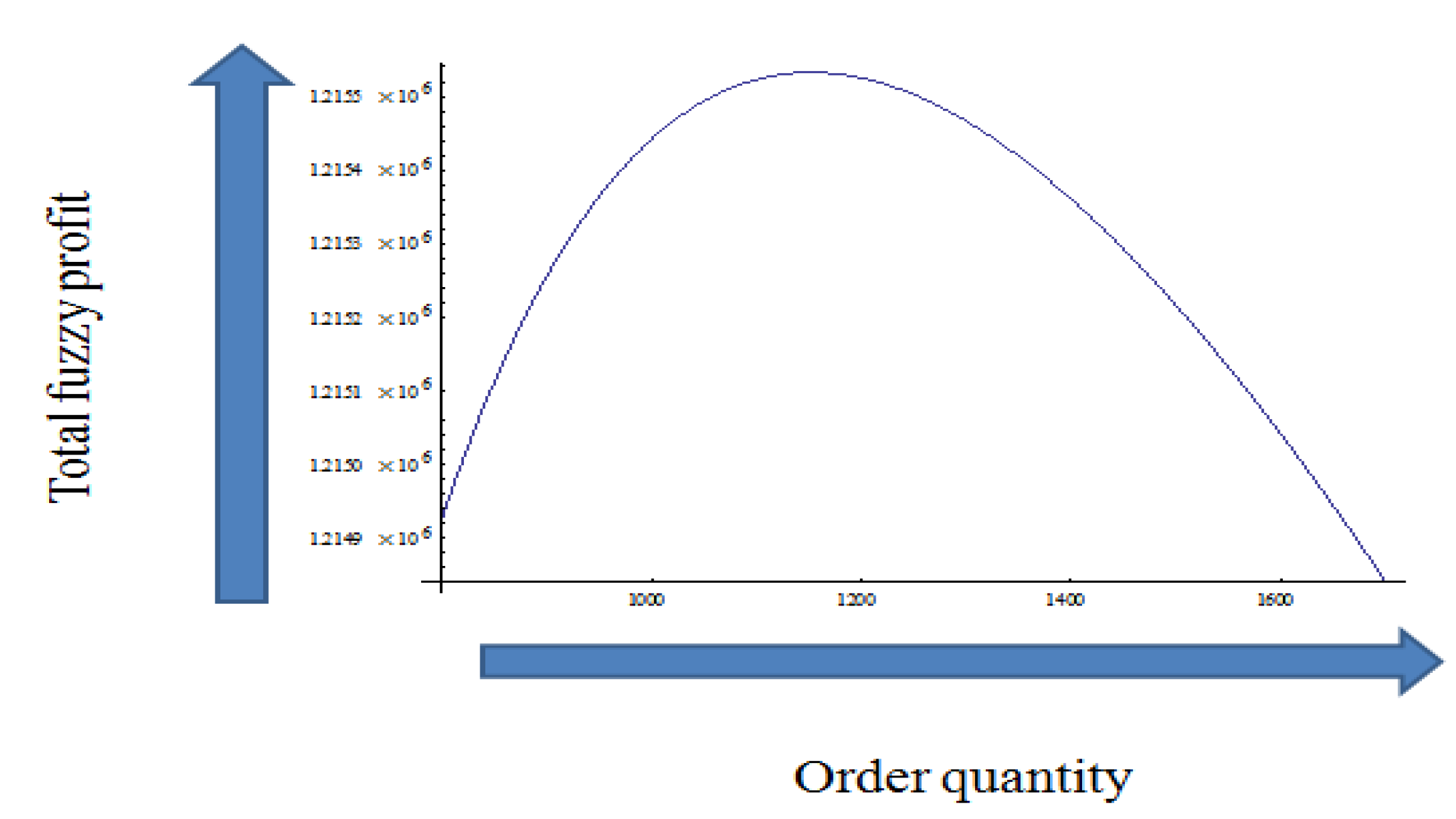
6. Formulation of the Total Profit Function under Fuzzy Environment

The decision maker studies each order and obtains more reliable evidence with respect to demand. Therefore, the decision maker is able to modify the deviation values (Bjork [56]) during the planning horizon based on what they have learned from the previous planning process. From this point of view, we considered that the demand is imprecise in nature and is treated as triangular fuzzy number, $\tilde{D}=\left(D-{\Delta }_l,D, D+{\Delta }_h\right)$ (Bjork [56]).

From Equation (2), we can obtain

$$d\left(\tilde{D},0\right)=\frac{1}{4}\left(D-{\Delta }_l+2D+D+{\Delta }_h\right)=D+\frac{1}{4}{\Delta }_h-\frac{1}{4}{\Delta }_l,$$

(10)

Scenario-1 under fuzzy environment.

• We can also obtain formulation of total profit function under fuzzy environment for the case of ($0\le M\le t_n\le T_n$).

Now, the fuzzification of the profit function from Equation (6) is as follows:

$$\begin{array}{l}{\tilde{\Psi }}_1\left(Q\right)=s\tilde{D}+\frac{vDp\left(n\right)}{1-p\left(n\right)}+\frac{\left(p{I}_e-c{I}_p\right){\tilde{D}}^2{M}^2}{2\left(1-p\left(n\right)\right)Q}-\frac{K\tilde{D}}{\left(1-p\left(n\right)\right)Q}\hfill \\ -\frac{(c+d-c_s{I}_{p}p\left(n\right)M-\left(c\tilde{D}{I}_p-c{I}_{p}M\tilde{D}p\left(n\right)M\right)}{1-p\left(n\right)}-\hfill \\ \frac{h\left[\left(\frac{{(1-p\left(n\right))}^2}{2\tilde{D}}+\frac{hp\left(n\right)}{\chi }\right)+\frac{c{(1-p\left(n\right))}^2{I}_p}{2\tilde{D}}+\frac{p\left(n\right)c_s{I}_p}{\chi }\right]Q\tilde{D}}{1-p\left(n\right)}.\hfill \end{array}$$

(11)

The defuzzification of fuzzy total profit per cycle is obtained from Equation (11):

$$\begin{array}{l}d\left({\tilde{\Psi }}_1\left(Q\right),0\right)=sd\left(\tilde{D},0\right)+\frac{vd\left(\tilde{D},0\right)p(n)}{1-p(n)}+\frac{{\left(d\left(\tilde{D},0\right)\right)}^2{M}^2(I_{e}p-I_{p}c)}{2(1-p(n))Q}-\frac{Kd\left(\tilde{D},0\right)}{(1-p(n))Q}\\ -\frac{(c+d-p\left(n\right)c_s{I}_{p}M-(1-p(n)M)I_{p}cd\left(\tilde{D},0\right)}{1-p(n)}-\\ \frac{h\left[\left(\frac{{(1-p(n))}^2}{2d\left(\tilde{D},0\right)}+\frac{hp(n)}{\chi }\right)+\frac{{(1-p(n))}^2{I}_{p}c}{2d\left(\tilde{D},0\right)}+\frac{p\left(n\right)c_s{I}_p}{\chi }\right]Qd\left(\tilde{D},0\right)}{1-p(n)}.\end{array}$$

(12)

The value of $d\left(\tilde{D},\hspace{0.17em}0\right)$ from Equation (10) substituted in (12) provides

$$\begin{array}{l}d\left({\tilde{\Psi }}_1\left(Q\right),0\right)={\tilde{\Psi }}_{21}\left(Q\right)=s\left(D+\frac{{\mathsf{\Delta }}_l}{4}-\frac{{\mathsf{\Delta }}_h}{4}\right)+\frac{v\left(D+\frac{{\mathsf{\Delta }}_l}{4}-\frac{{\mathsf{\Delta }}_h}{4}\right)p\left(n\right)}{1-p\left(n\right)}+\frac{{\left(\left(D+\frac{{\mathsf{\Delta }}_l}{4}-\frac{{\mathsf{\Delta }}_h}{4}\right)\right)}^2{M}^2\left(I_{e}p-I_{p}c\right)}{2\left(1-p\left(n\right)\right)Q}\hfill \\ -\frac{K\left(D+\frac{{\mathsf{\Delta }}_l}{4}-\frac{{\mathsf{\Delta }}_h}{4}\right)}{\left(1-p\left(n\right)\right)Q}-\frac{(c+d-c_{s}M{I}_{p}p\left(n\right)-\left(Mc{I}_p-c{I}_{p}p\left(n\right)M\right)\left(D+\frac{{\mathsf{\Delta }}_l}{4}-\frac{{\mathsf{\Delta }}_h}{4}\right)}{1-p\left(n\right)}\hfill \\ -\frac{h\left[\left(\frac{({(1-p\left(n\right))}^2}{\left(D+\frac{{\mathsf{\Delta }}_l}{4}-\frac{{\mathsf{\Delta }}_h}{4}\right)}+\frac{p\left(n\right)}{\chi }\right)+\frac{c{I}_p({(1-p\left(n\right))}^2}{\left(D+\frac{{\mathsf{\Delta }}_l}{4}-\frac{{\mathsf{\Delta }}_h}{4}\right)}+\frac{c_s{I}_{p}p\left(n\right)}{\chi }\right]Q\left(D+\frac{{\mathsf{\Delta }}_l}{4}-\frac{{\mathsf{\Delta }}_h}{4}\right)}{1-p\left(n\right)},\hfill \end{array}$$

(13)

Scenario-2, under fuzzy environment.

• We obtain the formulation of total profit function under fuzzy environment for the case of ($0\le t_n\le M\le T_n$).

Now, the fuzzification of the profit function is obtained from Equation (7):

$$\begin{gathered} {\tilde{\Psi }}_2\left(Q\right)=s\tilde{D}+\frac{\left[vp\left(n\right)+p\left(n\right)c_s{I}_e\left(M-t_n\right)-\left(d+c\right)+I_{p}cM\left(1-p\left(n\right)\right)\right]}{1-p\left(n\right)}\tilde{D}+\frac{{\tilde{D}}^2{M}^2\left(p{I}_e-c{I}_P\right)}{2\left(1-p\left(n\right)\right)Q} \\ -\frac{Q\left[h{(1-p\left(n\right))}^2\chi +2p\left(n\right)\tilde{D}+{(1-p\left(n\right))}^{2}c\chi I_p-2p\left(n\right)I_e\tilde{D}{c}_s\right]}{2\left(1-p\left(n\right)\right)\chi }-\frac{\tilde{D}K}{\left(1-p\left(n\right)\right)Q}. \end{gathered}$$

(14)

The defuzzification of fuzzy total profit per cycle is obtained from Equation (14):

$$\begin{array}{l}d\left({\tilde{\Psi }}_2\left(Q\right),0\right)=sd\left(\tilde{D},0\right)+\frac{\left[vp\left(n\right)+p\left(n\right)I_e{c}_s\left(M-t_n\right)-\left(d+c\right)+M{I}_p\left(1-p\left(n\right)\right)c\right]}{1-p\left(n\right)}d\left(\tilde{D},0\right)\hfill \\ +\frac{{(d\left(\tilde{D},0\right))}^2{M}^2\left(p{I}_e-c{I}_P\right)}{2\left(1-p\left(n\right)\right)Q}\hfill \\ -\frac{Q\left[\chi {(1-p\left(n\right))}^{2}h+2p\left(n\right)\tilde{D}+{(1-p\left(n\right))}^{2}c\chi I_p-2p\left(n\right)d\left(\tilde{D},0\right)I_e{c}_s\right]}{2\chi \left(1-p\left(n\right)\right)}-\frac{Kd\left(\tilde{D},0\right)}{\left(1-p\left(n\right)\right)Q} .\hfill \end{array}$$

(15)

The value of $d\left(\tilde{D},0\right)$ from Equation (10) substituted in (15) provides

$$\begin{gathered} d\left({\tilde{\Psi }}_2\left(Q\right),0\right)={\tilde{\Psi }}_{23}\left(Q\right)=s\left(D+\frac{{\mathsf{\Delta }}_l}{4}-\frac{{\mathsf{\Delta }}_h}{4}\right)+\frac{\left[vp\left(n\right)+p\left(n\right)I_e{c}_s\left(M-t_n\right)-\left(d+c\right)+M\left(1-p\left(n\right)\right)I_{p}c\right]}{1-p\left(n\right)}\left(D+\frac{{\mathsf{\Delta }}_l}{4}-\frac{{\mathsf{\Delta }}_h}{4}\right)+ \\ \frac{{\left(\left(D+\frac{{\mathsf{\Delta }}_l}{4}-\frac{{\mathsf{\Delta }}_h}{4}\right)\right)}^2{M}^2\left(p{I}_e-c{I}_P\right)}{2\left(1-p\left(n\right)\right)Q}-\frac{1}{2\chi \left(1-p\left(n\right)\right)}\left(\begin{array}{c}{(1-p\left(n\right))}^{2}h\chi +2\left(D+\frac{{\mathsf{\Delta }}_l}{4}-\frac{{\mathsf{\Delta }}_h}{4}\right)p\left(n\right)\\ +{(1-p\left(n\right))}^2\chi I_{p}c \\ -2\left(D+\frac{{\mathsf{\Delta }}_l}{4}-\frac{{\mathsf{\Delta }}_h}{4}\right)c_s{I}_{e}p\left(n\right)\end{array}\right)-\frac{K\left(D+\frac{{\mathsf{\Delta }}_l}{4}-\frac{{\mathsf{\Delta }}_h}{4}\right)}{\left(1-p\left(n\right)\right)Q}, \end{gathered}$$

(16)

Scenario-3 under fuzzy environment.

• We obtain the formulation of total profit function under fuzzy environment for the case of $\left(t_n\le T_n\le M\right)$.

Now, the fuzzification of profit function is obtained from Equation (8):

$$\begin{gathered} {\tilde{\Psi }}_3\left(Q\right)=s\tilde{D}+v\tilde{D}\frac{p\left(n\right)}{1-p\left(n\right)}+\frac{I_{e}p\left(1-p\left(n\right)\right)Q}{2}+\frac{c_s{I}_{e}p\left(n\right)\left(M-t_n\right)\tilde{D}}{1-p\left(n\right)}-\frac{K\tilde{D}}{\left(1-p\left(n\right)\right)Q}-\frac{\tilde{D}\left(d+c\right)}{1-p\left(n\right)} \\ -\frac{hQ[\left(1-p{(n)}^2\chi +2\tilde{D}p\left(n\right)\right]}{2\left(1-p\left(n\right)\right)\chi }+Mp{I}_e\tilde{D}-Q{I}_e\left(1-p\left(n\right)\right)p. \end{gathered}$$

(17)

The defuzzification of fuzzy total profit per cycle is obtained from Equation (17):

$$\begin{gathered} {\tilde{\Psi }}_3\left(Q\right)=s\tilde{D}+v\tilde{D}\frac{p\left(n\right)}{1-p\left(n\right)}+\frac{I_{e}p\left(1-p\left(n\right)\right)Q}{2}+\frac{c_s{I}_{e}p\left(n\right)\left(M-t_n\right)\tilde{D}}{1-p\left(n\right)}-\frac{K\tilde{D}}{\left(1-p\left(n\right)\right)Q}-\frac{\tilde{D}\left(d+c\right)}{1-p\left(n\right)} \\ -\frac{hQ[\left(1-p{(n)}^2\chi +2\tilde{D}p\left(n\right)\right]}{2\left(1-p\left(n\right)\right)\chi }+Mp{I}_e\tilde{D}-Q{I}_e\left(1-p\left(n\right)\right)p. \end{gathered}$$

(18)

The value of $d\left(\tilde{D},0\right)$ from Equation (10) substituted in (18) provides

$$\begin{array}{l}d\left({\tilde{\Psi }}_3\left(Q,\hspace{0.17em}0\right)\right)={\tilde{\Psi }}_{23}\left(Q\right)=\\ s\left(D+\frac{{\Delta }_l}{4}-\frac{{\Delta }_h}{4}\right)+v\left(D+\frac{{\Delta }_l}{4}-\frac{{\Delta }_h}{4}\right)\frac{p(n)}{1-p(n)}+\frac{I_{e}p(1-p(n))Q}{2}\\ +\frac{c_s{I}_{e}p(n)(M-t_n)\left(D+\frac{{\Delta }_l}{4}-\frac{{\Delta }_h}{4}\right)}{1-p(n)}-\frac{K\left(D+\frac{{\Delta }_l}{4}-\frac{{\Delta }_h}{4}\right)}{(1-p(n))Q}-\frac{(c+d)\left(D+\frac{{\Delta }_l}{4}-\frac{{\Delta }_h}{4}\right)}{1-p(n)}\\ -\hspace{0.17em}\frac{\hspace{0.17em}h\hspace{0.17em}Q\left[{(1-p(n))}^2\chi +2p(n)\left(D+\frac{{\Delta }_l}{4}-\frac{{\Delta }_h}{4}\right)\right]}{2(1-p(n))\chi }+p{I}_e\left(D+\frac{{\Delta }_l}{4}-\frac{{\Delta }_h}{4}\right)M-p{I}_e(1-p(n))Q\\ \hspace{0.17em}\end{array}$$

(19)

Now, the summarized retailer’s profit for each scenario is as follows:

$${\tilde{\Psi }}_F\left(Q\right)=\{\begin{array}{l}{\tilde{\Psi }}_{21}\left(Q\right),\hspace{0.17em}\hspace{0.17em}\hspace{0.17em}\hspace{0.17em}\hspace{0.17em}\hspace{0.17em}{T}_n\ge t_n\ge M\hspace{0.17em}\hspace{0.17em}\hspace{0.17em}\mathrm{For}\hspace{0.17em}\hspace{0.17em}\mathrm{scenario}\hspace{0.17em} -1\hspace{0.17em}\hspace{0.17em}\hspace{0.17em}\\ {\tilde{\Psi }}_{22}\left(Q\right),\hspace{0.17em}\hspace{0.17em}\hspace{0.17em}\hspace{0.17em}\hspace{0.17em}\hspace{0.17em}\hspace{0.17em}{T}_n\ge M\ge t_n\hspace{0.17em}\hspace{0.17em}\hspace{0.17em}\mathrm{For}\hspace{0.17em}\hspace{0.17em}\mathrm{scenario}\hspace{0.17em}\hspace{0.17em}-2\hspace{0.17em}\hspace{0.17em}\hspace{0.17em}\hspace{0.17em}\hspace{0.17em}\\ {\tilde{\Psi }}_{32}\left(Q\right),\hspace{0.17em}\hspace{0.17em}\hspace{0.17em}\hspace{0.17em}\hspace{0.17em}\hspace{0.17em}\hspace{0.17em}M\ge T\ge t_n\hspace{0.17em}\hspace{0.17em}\hspace{0.17em}\hspace{0.17em}\mathrm{For}\hspace{0.17em}\hspace{0.17em}\mathrm{scenario}\hspace{0.17em}\hspace{0.17em}-3\hspace{0.17em}\hspace{0.17em}\hspace{0.17em}\end{array}$$

(20)

6.1. Solution Method

For optimal value of total fuzzy profit function ${\tilde{\Psi }}_{21}\left(Q\right)$,$\frac{d{\tilde{\Psi }}_{21}\left(Q\right)}{dQ}=\hspace{0.17em}\hspace{0.17em}0$, obtaining $Q=Q_1{}^{\ast }$ which is equal to $Q_1{}^{\ast }=\sqrt{\frac{[2K-\tilde{D}{M}^2(I_{e}p-c{I}_p)]\tilde{D}\chi }{h({(1-p(n))}^2\chi +2.\tilde{D}p(n))+\chi c{I}_p{(1-p(n))}^2+2\tilde{D}{c}_s{I}_{p}p(n)}}$ using Equation (13). Now, having calculated second derivative of total fuzzy profit function and replaced the value of $Q_1{}^{\ast }$ and simplified it with the mathematical software, we obtained $d^2{\Psi }_{21}(Q_1{}^{\ast })/d{Q}^2<0\hspace{0.17em},\hspace{1em}\forall Q_1{}^{\ast }>0$, which represents the $Q_1{}^{\ast }$ as an optimal value of the total fuzzy profit function ${\tilde{\Psi }}_{21}\left(Q\right)$. The optimal buyer’s profit per cycle for Scenario-1 is ${\tilde{\Psi }}_{21}\left(Q_1{}^{\ast }\right)=\frac{T{R}_1-T{C}_1}{T_n}$. The optimal buyer’s profit for scenario-2 and scenario-3 can be calculated in a similar way. The optimal buyer’s profit ${\tilde{\Psi }}_{22}\left(Q_2{}^{\ast }\right)=\frac{T{R}_2-T{C}_2}{T_n}$, where $Q_2{}^{\ast }=\sqrt{\frac{2K\tilde{D}\chi -{\tilde{D}}^2{M}^2\chi (p{I}_e-c{I}_P)}{h\left((1-p{(n)}^2\chi +2\tilde{D}p(n)\right)+\chi c{I}_p{(1-p(n))}^2-2\tilde{D}{c}_s{I}_{e}p(n)}}$ for Scenario-2 using Equation (16) and the optimal buyer’s profit for Scenario-3 ${\tilde{\Psi }}_{23}\left(Q_3{}^{\ast }\right)=\frac{T{R}_3-T{C}_3}{T_n}$, where $Q_3{}^{\ast }=\sqrt{\frac{2K\tilde{D}\chi }{2c_s{I}_{e}p(n)\tilde{D}+h((1-p{(n)}^2)\chi +2\tilde{D}p\left(n\right))+p{I}_e\chi {(1-p(n))}^2}\hspace{0.17em}}$ using Equation (19). The proof of concavity for the buyer’s total profit for Scenario-1, Scenario-2 and Scenario-3 under fuzzy environment is represented graphically in the Figure 7, Figure 8 and Figure 9 below.

6.2. Algorithm

To compute the problem stated here, the algorithm method of Shinn and Hwang [17] needs to be implemented.

Step 1. Insert all inventory parameters which are known $[D,\hspace{0.17em}\tilde{D},I_e,I_p,p,d,k,h,n,p\left(n\right),\hspace{0.17em}M,{\Delta }_l,{\Delta }_h,b,\hspace{0.17em}\hspace{0.17em}\lambda ]$ in Equations (13), (16) and (19).

Step 2. Now, calculate $Q^{\ast }=Q_1$ with the help of the solution method and substituting in Equations (9) and (10) to determine $T_n$ and $t_n$. If $M\le t_n\le T_n$, then determine retailer’s profit concerning this Scenario-1 from Equation (13).

Step 3. Now, calculate $Q_2{}^{\ast }=Q_2$ with the help of the solution method and substituting in Equations (9) and (10); then, determine $T_n$ and $t_n$. If $t_n\le M\le T_n$, then determine retailer’s profit concerning this Scenario-2 from Equation (16).

Step 4. Now, calculate $Q_3{}^{\ast }=Q_3$ with the help of the solution method and substituting in Equations (9) and (10); then, determine $T_n$ and $t_n$. If $t_n\le T_n\le M$, then determine retailer’s profit concerning this Scenario-3 from Equation (19).

Step 5. In this step, compare the lot size and buyer’s profit in all scenarios and also determine the circumstances under which the profit is better for seller and buyer. Regarding the scenarios, they are all explained in the discussion part.

6.3. Observations

In this section, with the help of algorithms to a certain extent, we discussed and analyzed the defined scenario and also attempted to decide which case is superior for this model. In Scenario-1, fuzzy environment has not been considered due to lesser trade credit period and the absence of benefit for buyers. Due to reduced trade credit period, the seller cannot sell more items and finally gains less profit. In Scenario-2 under fuzzy environment, the buyer receives a suitable trade credit period as compared Scenario-1 under fuzzy environment, and therefore can earn more profit. This scenario is beneficial for the buyer and the seller due to suitable trade credit periods. If we consider Scenario-3 under a fuzzy environment, it is not beneficial for sellers due to long trade credit periods, which can lead to the sellers facing more risk. On the account of this, the seller does not provide more credit period to the buyer. For this reason, this scenario was not considered. Finally, we considered Scenario-2 in this model for sensitivity analysis and the comparison of total fuzzy profit has been shown in the Figure 10.

6.4. Numerical Example

• Numerical example for crisp environment.

Input parameters have been obtained from Jayaswal et al. [42] for this proposed model, which are as follows:

$\begin{array}{l}D=50000\hspace{0.17em}\hspace{0.17em}\mathrm{units}\hspace{0.17em}\hspace{0.17em}\mathrm{per}\hspace{0.17em}\mathrm{year},\hspace{0.17em}\lambda =1752000\hspace{0.17em}\hspace{0.17em}\hspace{0.17em}\mathrm{units}\hspace{0.17em}\hspace{0.17em}\mathrm{per}\hspace{0.17em}\hspace{0.17em}\mathrm{year},p=\$\hspace{0.17em}50\hspace{0.17em}\hspace{0.17em}\mathrm{per}\hspace{0.17em}\hspace{0.17em}\mathrm{unit},\hspace{0.17em}\\ d=\$\hspace{0.17em}0.5\hspace{0.17em}\hspace{0.17em}\mathrm{per}\hspace{0.17em}\hspace{0.17em}\mathrm{unit},\hspace{0.17em}{C}_p=\$25\hspace{0.17em}\mathrm{per}\hspace{0.17em}\hspace{0.17em}\mathrm{unit},h=\$5/\mathrm{unit}/\mathrm{year},\hspace{0.17em}\hspace{0.17em}{I}_e=0.10\hspace{0.17em}\mathrm{per}\hspace{0.17em}\hspace{0.17em}\mathrm{year},\\ I_p=0.15\hspace{0.17em}\mathrm{per}\hspace{0.17em}\hspace{0.17em}\mathrm{year},b=0.7932,n=5,\hspace{0.17em}p\left(n\right)=0.039\hspace{0.17em},M=0.15\hspace{0.17em}\hspace{0.17em}\mathrm{yea}r.\hspace{0.17em}{T}_n{}^{\ast }=0.025\hspace{0.17em}\mathrm{year},\hspace{0.17em}\hspace{0.17em}\\ t_n{}^{\ast }=0.0076\mathrm{year},\hspace{0.17em}{Q}^{\ast }=1336\hspace{0.17em}\hspace{0.17em}\hspace{0.17em}\mathrm{unit}\hspace{0.17em}\hspace{0.17em}\mathrm{and}\hspace{0.17em}\hspace{0.17em}{\Psi }_1\left(Q^{\ast }\right)=1206930\hspace{0.17em}\$\end{array}$

• Numerical example under fuzzy environment.

$\begin{array}{l}D=50000\hspace{0.17em}\hspace{0.17em}\mathrm{units}\hspace{0.17em}\hspace{0.17em}\mathrm{per}\hspace{0.17em}\mathrm{year},\tilde{D}=\left(44000,\hspace{0.17em}50000,\hspace{0.17em}62000\right)\hspace{0.17em},{\Delta }_l=6000,{\Delta }_h=12000,p=\$\hspace{0.17em}50\hspace{0.17em}\hspace{0.17em}\mathrm{per}\hspace{0.17em}\hspace{0.17em}\mathrm{unit},\\ \lambda =175000\hspace{0.17em}\hspace{0.17em}\hspace{0.17em}\mathrm{units}\hspace{0.17em}\hspace{0.17em}\mathrm{per}\hspace{0.17em}\hspace{0.17em}\mathrm{year},,\hspace{0.17em}d=\$\hspace{0.17em}0.5\hspace{0.17em}\hspace{0.17em}\mathrm{per}\hspace{0.17em}\hspace{0.17em}\mathrm{unit},\hspace{0.17em}{C}_p=\$25\hspace{0.17em}\mathrm{per}\hspace{0.17em}\hspace{0.17em}\mathrm{unit},h=\$5/\mathrm{unit}/\mathrm{year},\hspace{0.17em}\hspace{0.17em}\\ I_e=0.10\hspace{0.17em}\mathrm{per}\hspace{0.17em}\hspace{0.17em}\mathrm{year},I_p=0.15\hspace{0.17em}per\hspace{0.17em}\hspace{0.17em}\mathrm{year},b=0.7932,n=5,\hspace{0.17em}p\left(n\right)=0.039,\end{array}$

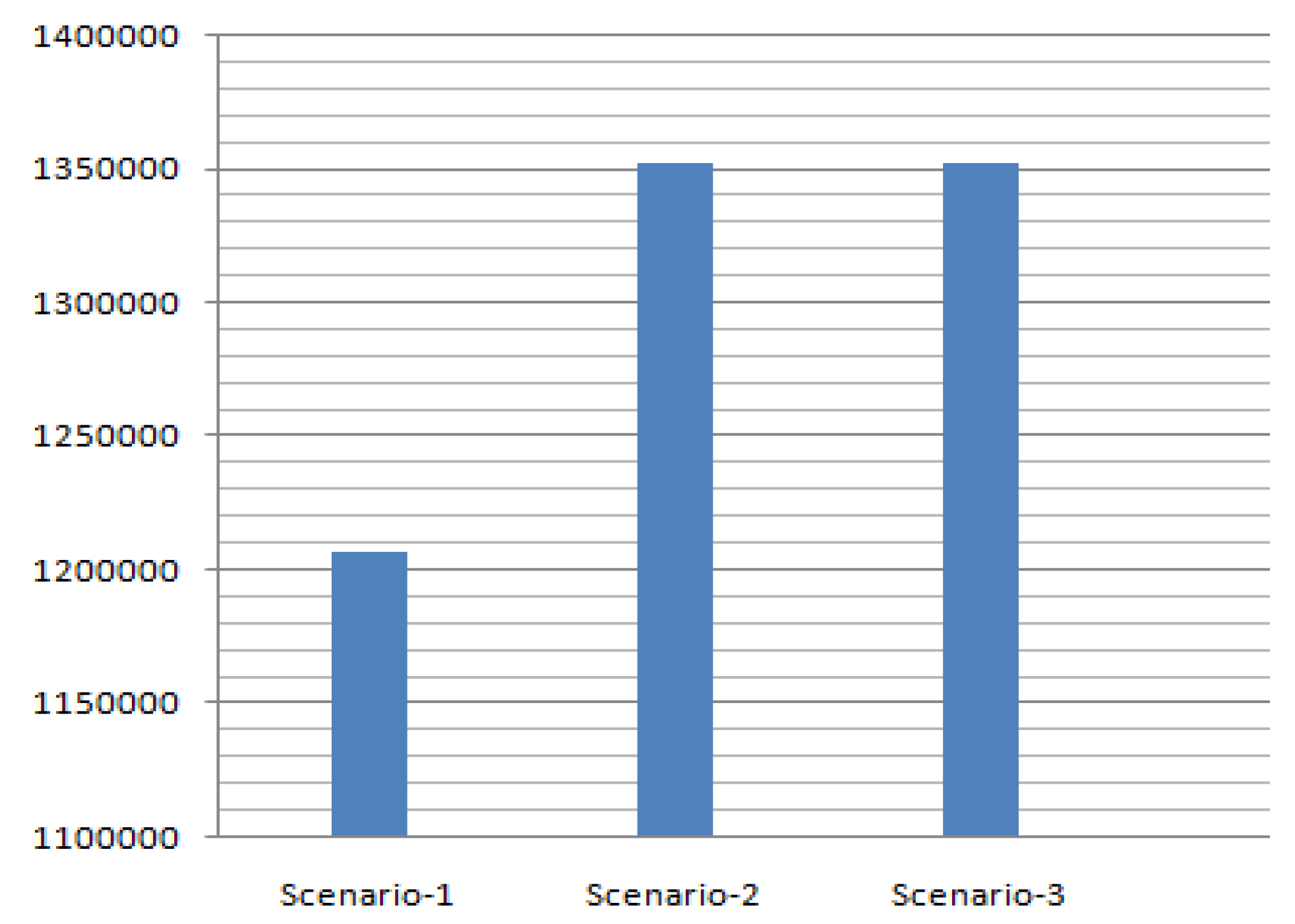
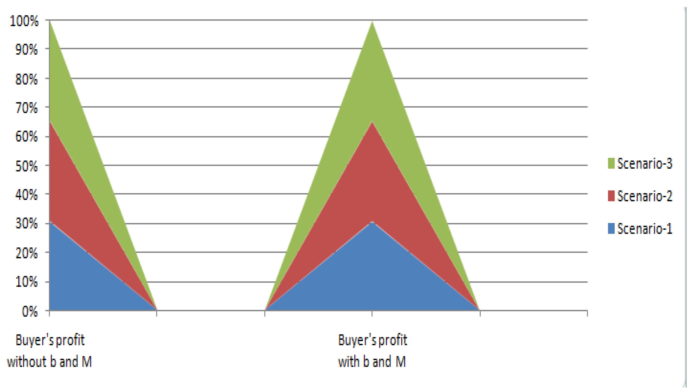
• Numerical example for Scenario-1 with above data under fuzzy environment.

The buyer’s optimal order quantity, total fuzzy profit, cycle length and screening time are the following:

$M=0.008\hspace{0.17em}\hspace{0.17em}\mathrm{year}.,\hspace{0.17em}{T}_n{}^{\ast }=0.024\mathrm{year},\hspace{0.17em}\hspace{0.17em}{t}_n{}^{\ast }=0.008\hspace{0.17em}\mathrm{year},\hspace{0.17em}{Q}^{\ast }=1390\hspace{0.17em}\hspace{0.17em}\hspace{0.17em}\mathrm{unit}\hspace{0.17em}\hspace{0.17em}\mathrm{and}\hspace{0.17em}\hspace{0.17em}{\Psi }_{21}\left(Q^{\ast }\right)=1207120\hspace{0.17em}\$$.

If there is no learning and no trade credit policy in this scenario, it means that $b=0\hspace{0.17em}\hspace{0.17em}\mathrm{and}\hspace{0.17em}\hspace{0.17em}\hspace{0.17em}M=0$.

In the above numerical example, then, the buyer’s optimal order quantity, total fuzzy profit, cycle length and screening time are

$T_n{}^{\ast }=0.027\hspace{0.17em}\mathrm{year},\hspace{0.17em}\hspace{0.17em}{t}_n{}^{\ast }=0.008\hspace{0.17em}\mathrm{year},\hspace{0.17em}{Q}^{\ast }=1455\hspace{0.17em}\hspace{0.17em}\hspace{0.17em}\mathrm{unit}\hspace{0.17em}\hspace{0.17em}\mathrm{and}\hspace{0.17em}\hspace{0.17em}{\tilde{\Psi }}_{21}\left(Q^{\ast }\right)=1206380\$$.

• Numerical example for Scenario-2 with above data under fuzzy environment.

The buyer’s optimal order quantity, total fuzzy profit, cycle length and screening time are

$M=0.0136\hspace{0.17em}\hspace{0.17em}\mathrm{year}.\hspace{0.17em}{T}_n{}^{\ast }=0.027\hspace{0.17em}\mathrm{year},\hspace{0.17em}\hspace{0.17em}{t}_n{}^{\ast }=0.0079\hspace{0.17em}\mathrm{year},\hspace{0.17em}{Q}^{\ast }=1396\hspace{0.17em}\hspace{0.17em}\hspace{0.17em}\mathrm{unit}\hspace{0.17em}\hspace{0.17em}\mathrm{and}\hspace{0.17em}\hspace{0.17em}{\Psi }_{21}\left(Q^{\ast }\right)=1352850\hspace{0.17em}\$$.

If there is no learning and no trade credit policy in this scenario, it means that $b=0\hspace{0.17em}\hspace{0.17em}\mathrm{and}\hspace{0.17em}\hspace{0.17em}\hspace{0.17em}M=0$.

In the above numerical example, then, buyer’s optimal order quantity, total fuzzy profit, cycle length and screening time are

$\hspace{0.17em}{T}_n{}^{\ast }=0.026\hspace{0.17em}\mathrm{year},\hspace{0.17em}\hspace{0.17em}{t}_n{}^{\ast }=0.0087\hspace{0.17em}\mathrm{year},\hspace{0.17em}{Q}^{\ast }=1535\hspace{0.17em}\hspace{0.17em}\hspace{0.17em}\mathrm{unit}\hspace{0.17em}\hspace{0.17em}\mathrm{and}\hspace{0.17em}\hspace{0.17em}{\tilde{\Psi }}_{22}\left(Q^{\ast }\right)=1352220\$$.

• Numerical example for Scenario-3 with above data under fuzzy environment.

The buyer’s optimal order quantity, total fuzzy profit, cycle length and screening time are

$M=20/365\hspace{0.17em}\hspace{0.17em}\mathrm{year}.\hspace{0.17em}{T}_n{}^{\ast }=8/365\hspace{0.17em}\mathrm{year},\hspace{0.17em}\hspace{0.17em}{t}_n{}^{\ast }=3/365\hspace{0.17em}\mathrm{year},\hspace{0.17em}{Q}^{\ast }=1399\hspace{0.17em}\hspace{0.17em}\hspace{0.17em}\mathrm{unit}\hspace{0.17em}\hspace{0.17em}\mathrm{and}\hspace{0.17em}\hspace{0.17em}{\Psi }_{21}\left(Q^{\ast }\right)=1352865\hspace{0.17em}\$$.

If there is no learning and no trade credit policy, it means that $b=0\hspace{0.17em}\hspace{0.17em}\mathrm{and}\hspace{0.17em}\hspace{0.17em}\hspace{0.17em}M=0$ and its effect have been shown in the Figure 11. In the above numerical example, the optimal order quantity, total fuzzy profit, cycle length and screening time are given below.

$T_n{}^{\ast }=0.030\hspace{0.17em}\mathrm{year},\hspace{0.17em}\hspace{0.17em}{t}_n{}^{\ast }=0.0089\hspace{0.17em}\mathrm{year},\hspace{0.17em}{Q}^{\ast }=1566\hspace{0.17em}\hspace{0.17em}\hspace{0.17em}\mathrm{unit}\hspace{0.17em}\hspace{0.17em}\mathrm{and}\hspace{0.17em}\hspace{0.17em}{\tilde{\Psi }}_{23}\left(Q^{\ast }\right)=1352345\hspace{0.17em}\$$.

From Scenario-1, Scenario-2 and Scenario-3, the effect of the presence and absence of learning and credit financing for buyers is visible. There are more changes in the buyer’s optimal order quantity, total fuzzy profit, cycle length and screening time due to the absence of learning and credit policy. Here, it can be easily seen that buyers received a larger order quantity but less profit as compared to the scenario model with the effect of leaning under credit policy. Finally, buyers gained less profit in the absence of credit financing policy and the effect of the learning concept in this scenario. The learning effect and credit policy provided a positive effect in this scenario and the comparison of crisp and fuzzy environment have been shown in the

Table 2. Comparison of crisp and fuzzy environment.

Model	Optimal Cycle Length (Yr.) ${\mathit{T}}_{\mathit{n}}{}^{\ast }$	Optimal Screening Time (Yr.) ${\mathit{t}}_{\mathit{n}}{}^{\ast }$	Optimal Cycle Length ${\mathit{Q}}^{\ast }$	Buyer’s Total Profit ($)
Crisp environment	0.0251	0.0076	1336	1,206,930
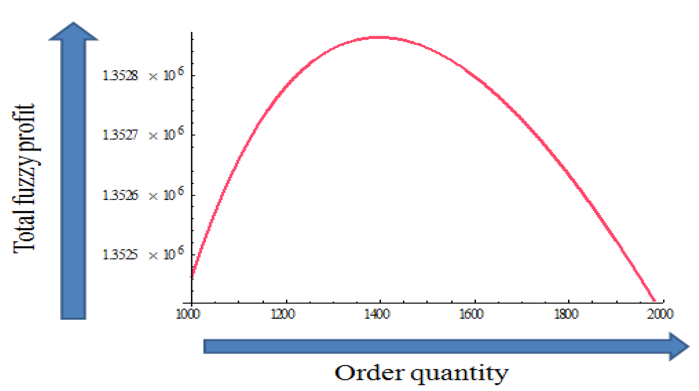
Fuzzy environment	0.0239	0.0079	1396	1,352,850

.

6.5. Sensitivity Analysis

Sensitivity analysis is accomplished to determine the hardiness of the model on affected parameters.

• Impact of trade credit

Table 3. Effect of financing period of time on lots, inspection time and buyer’s profit under learning effect.

Financing Period Time M (Year)	Inspection Time ${\mathit{t}}_{\mathit{n}}$(Year)	Buyer’s Optimal Length of Cycle ${\mathit{T}}_{\mathit{n}}$(Year)	Buyer’s Optimal Lots (Units)	Buyer’s Total Fuzzy Profit ${\tilde{\mathbf{\Psi }}}_{21}\left({\mathit{Q}}^{\ast }\right)$($)
4	0.0084	0.0328	1472	1,352,420
5	0.0079	0.0239	1396	1,352,850
8	0.0072	0.0223	1270	1,353,530

reveals the circumstances of trade credit profit operation acceptable by the buyer on the optimal solution. When the trade credit period along with the buyer’s profit increases, inspection time and lot size decrease; however, cycle length changes when credit period is exactly 0.021 years or is otherwise fixed. This indicates that the buyer ought to query for a long credit period from the seller in order to increase their profit.

• Impact of learning

From

Table 4. Effect of learning rate on order quantity, inspection time and buyer’s profit under learning effect.

Learning Rate $\mathit{b}$	Inspection Time ${\mathit{t}}_{\mathit{n}}$(Year)	Buyer’s Optimal Length of Cycle ${\mathit{T}}_{\mathit{n}}$(Year)	Buyer’s Optimal Lots ${\mathit{Q}}^{\ast }$(Units)	Buyer’s Total Fuzzy Profit ${\tilde{\mathbf{\Psi }}}_{21}\left({\mathit{Q}}^{\ast }\right)$($)
0.79	0.0079	0.0239	1396	1,352,850
0.80	0.0079	0.0239	1396	1,352,890
0.90	0.0079	0.0239	1395	1,353,290
1.00	0.0079	0.0239	1394	1,353,910
1.10	0.0079	0.0239	1392	1,354,790
1.20	0.0079	0.0238	1389	1,355,980

, it can be observed that if the learning rate rises from 0.79 to 1.20, then the buyer’s profit increases and the order quantity decreases while inspection time and cycle length are nearly fixed. This provides more information to the decision maker, and it helps them to earn more profit for the company. Consequently, the buyer obtains more information for the exercise of shipment.

• Impact of shipments

Table 5. Effect of shipment on lot, inspection time and buyer’s profit.

Number of Shipments $\mathit{n}$	Inspection Time ${\mathit{t}}_{\mathit{n}}$(Year)	Buyer’s Optimal Length of Cycle ${\mathit{T}}_{\mathit{n}}$(Year)	Buyer’s Optimal Lots ${\mathit{Q}}^{\ast }$(Units)	Buyer’s Total Fuzzy Profit ${\tilde{\mathbf{\Psi }}}_{21}\left({\mathit{Q}}^{\ast }\right)$($)
1	0.079	0.0239	1398	1,352,230
2	0.079	0.0239	1398	1,352,260
3	0.079	0.0239	1398	1,352,340
4	0.079	0.0239	1397	1,352,500
5	0.079	0.0239	1396	1,352,850

shows that the aggregate of shipment increases from 1 to 5 and the next order quantity initially drops to 5th shipment due to the separation of defective items from the lot, and after the 5th shipment, it declines steadily; numerically, we can say that it remains fixed. The buyer’s total profit increases when the number of shipments increases while inspection time and cycle time are almost fixed. It is advised that the buyer manages their profit with respect to shipments. The intensity level of the buyer’s benefit is not attained until 5th shipment, whereas it can be reached in the 5th shipment if the learning rate is 0.79.

• Impact of lower and upper fuzzy deviation on demand rate

Table 6. Effect of lower fuzzy and upper fuzzy for demand on order quantity, inspection time and buyer’s profit under learning effect.

Lower Fuzzy $\left({\mathbf{\Delta }}_{\mathit{l}}\right)$	Upper Fuzzy $\left({\mathbf{\Delta }}_{\mathit{h}}\right)$	Fuzzy Demand Rate $\tilde{\mathit{D}}$	Inspection Time ${\mathit{t}}_{\mathit{n}}$(year)	Buyer’s Optimal Length of Cycle ${\mathit{T}}_{\mathit{n}}$(year)	Buyer’s Optimal Lots $\mathit{Q}$(units)	Buyer’s Total Fuzzy Profit ${\tilde{\mathbf{\Psi }}}_{21}\left(\mathit{Q}\right)$($)
1000	2000	(49,000, 50,000, 52,000)	0.0076	0.0253	1345	1,231,720
2000	4000	(48,000, 50,000, 54,000)	0.0077	0.0250	1355	1,255,950
4000	8000	(46,000, 50,000, 58,000)	0.0078	0.0245	1376	1,304,400
5000	10,000	(45,000, 50,000, 60,000)	0.0079	0.0242	1386	1,328,630
6000	12,000	(44,000, 50,000, 62,000)	0.0079	0.0239	1396	1,352,850

shows that when the lower and upper fuzzy deviation of demand rate increases, the buyer’s total fuzzy profit and order quantity, as well as the time of inspection, increase. However, the length of the cycle decreases because the demand rate increases.

7. Comparison of Numerical Results of Related Inventory Models

In this paper, we proposed and inventory model for defective items, trade credit policy, and the effect of learning and fuzzy environment. In

Table 7. Comparison of results with our proposed model.

Authors	Contribution Details	Screening Time	Cycle Time	Order Quantity	Total Profit
Salameh and Jaber (2000) [57]	Lot sizing, EPQ/EOQ, screening cost/time and imperfect quality	-	-	1439 units	USD 1,212,235
Chang [61]	Inventory, imperfect quality, fuzzy set and signed distance	-	-	1429 units	USD 121,366.72
Yu et al. [58]	EOQ, deterioration, imperfect quality and partial backordering	-	0.0272 year	Order quantity, 1288 units Backorder quantity, 28 units	USD 1,212,148
Chung and Huang [62]	Lot sizing, EOQ, screening cost/time and Imperfect quality and trade credit policy.	0.009839 year	0.055 year	196 units	USD 346,583.3
Eroglu and Ozdemir [59]	Lot sizing, EOQ, screening cost/time and Imperfect quality and backorder	-	-	Order quantity, 2129 units Backorder quantity, 595 units	USD 341,116.89
Jaber et al. [25]	Lot sizing, EOQ, screening cost/time and imperfect quality and learning	-	-	1440 units	USD 1,217,452
Khan et al. [26]	EOQ, imperfect items, learning in screening, forgetting	-	-	2201 units (Lost sales) 2112 units (Backorders)	USD 1,222,394 USD 1,222,757
Jaggi and Mittal [63]	Inventory, imperfect items, deterioration and inspection	0.0073 year	0.025 year	1283 units	USD 1,224,183
Konstantaras et al. [31]	Inventory, EOQ, imperfect quality, learning effects and shortage	-	4.5 year	666 units	USD 68,985
Jaggi et al. [22]	Inventory, Imperfect items, shortages and permissible delay	0.0274 year	0.104 year	Order quantity, 1642 units Backorder quantity, 674 units	USD 347,086
Sulak [64]	Economic order quantity, defective items, backorder, graded mean integration representation method, trapezoidal/triangular fuzzy numbers	-	-	Order quantity, 2149 units Backorderquantity,594.53 units	USD 341,121.2
Shekarian et al. [65]	EOQ model, imperfect quality, holding cost, learning effect, triangular fuzzy number, graded mean integration value method	-	-	5000 units	USD 11,000,000
Khanna et al. [66]	Imperfect quality items, deterioration, shortages, price-dependent demand and credit financing	-	-	Order quantity,899 units Backorder quantity,283 units	USD 707,837
Patro et al. [40]	Inventory; economic order quantity, EOQ; imperfect quality, deteriorating items, proportionate discount, triangular fuzzy number, signed distance, learning effects and defuzzification	-	-	1117 Units	USD 1,273,420
Kazemi et al. [67]	EOQ, sustainability, carbon emission, imperfect quality, learning and inspection error	-	-	734 unit (without learning) and 713 units with learning	USD 1,184,628 without learning and USD 1,196,862 with learning
Jayaswal et al. [42]	EPQ, learning effects, imperfect items and trade-credit financing	0.0076 year	0.025 year	1336 units	USD 1,206,930
Rajeswari and Sugapriya [68]	EOQ, fuzzy, imperfect quality and repair	-	-	3423 units	USD 1,197,300
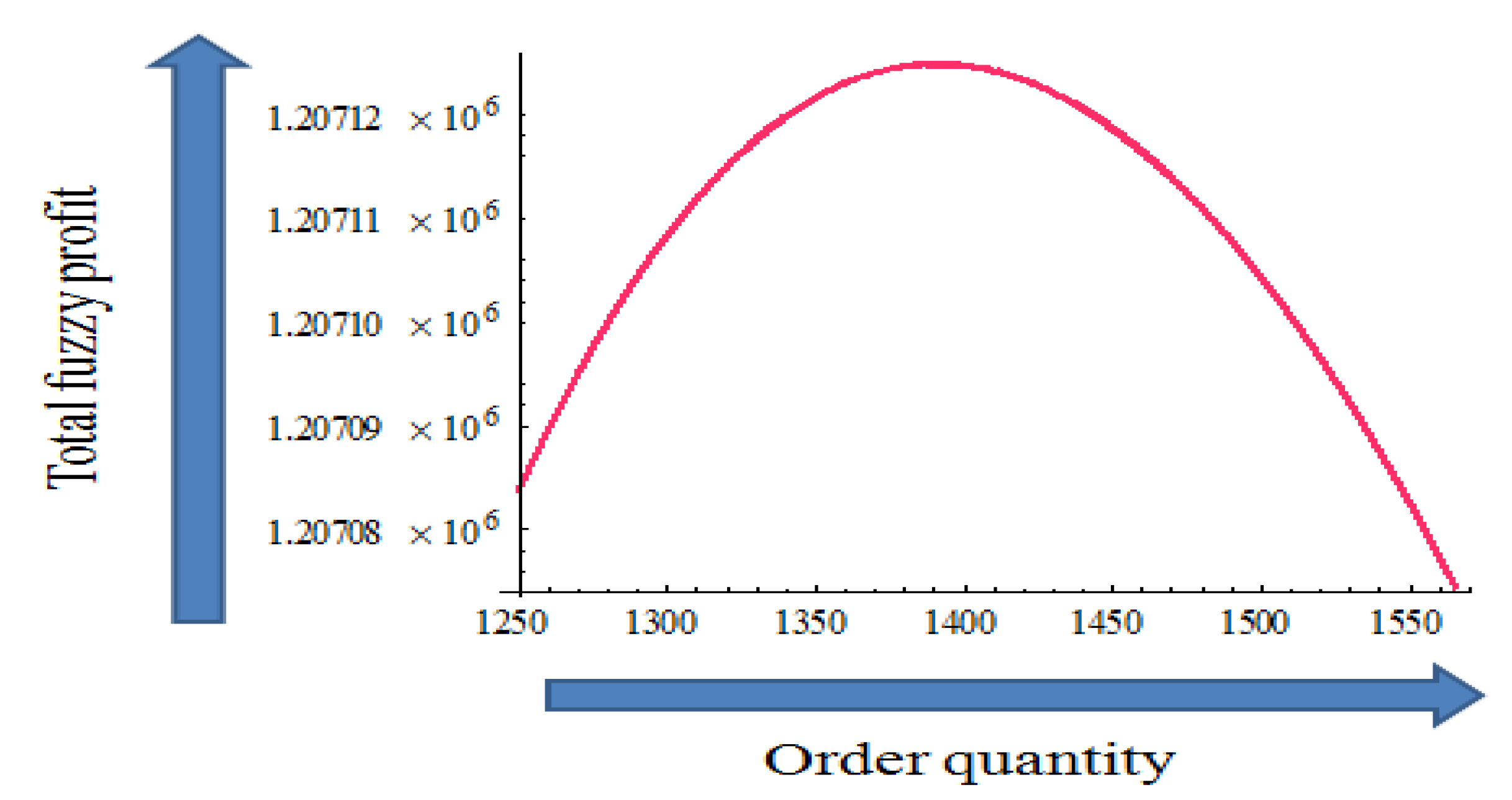
Tahami and Fakhravar [69]	Inventory, imperfect quality, order overlapping, graded mean integration, triangular fuzzy number and screening	-	-	1295 units	USD 1,212,072
Jayaswal et al. [47]	Learning impact, deterioration, defective quality item and trade credit financing policy	0.0214 year	0.0690 year	3756 units	USD 1,142,850
Alamri et al. [60]	Learning impact, deterioration, defective quality item and inflation	0.2752 year	1.0094 year	48,225 units	USD 1,662,440
Our paper	EOQ, defective items, learning effects, trade-credit, supply chain, triangular fuzzy number, fuzzy environment	0.0079 year	0.0214 year	1396 units	USD 1,352,850

, we compared our results with various published results. After comparison with the related published work, it was determined that our paper generated good results in the given scenarios. It was also determined that the inventory model for defective items with trade credit, learning and fuzzy environment has not been proposed before. Jayaswal et al. [47] developed inventory model with fuzzy environment for deteriorating imperfect quality items and considered the same data for numerical calculations. In Jayaswal et al. [47], cycle length is high compared to our model, and order quantity is also high. In our model, cycle length is low, so that the retailer can order frequently, receive low order quantity and generate the benefit of lesser holding cost. Further, Jayaswal et al. [42] proposed an inventory model for defective items with trade credit period. Results revealed that best case of trade credit provides maximum profit. Compared to our paper, Jayaswal et al. [42] did not consider learning and fuzzy environment which are more realistic concepts providing best results. Some inventory models were also developed with back ordering and partial back ordering (Yu et al. [58] and Eroglu and Ozdemir [59]); results are provided in Table 7. Alamri et al. [60] proposed inventory model without fuzzy environment and considered high deterministic demand.

After comparing with most of the papers provided n Table 7, it was determined that we have considered more realistic concepts, and sensitivity analysis also shows positive results.

8. Conclusions

This paper explains the buyer’s ordering policy with the effect of learning for defective items under a fuzzy environment and credit financing where the demand rate is imprecise in nature. The novelty of this paper is that the imprecise nature of demand rate can be manageable by a fuzzy environment, and can also maximize the buyer’s profit with the help of credit financing policy and learning effects. Moreover, the buyer’s profit is compared under crisp and fuzzy environments and the buyer gains more profit in a fuzzy environment compared to a crisp environment as shown in Table 2. It can be said that the fuzzy environment has a positive effect on the buyer’s ordering policy. Further, the learning rate and credit period affect the buyer’s total profit in a fuzzy environment. In the presence of learning and trade credit, buyers gain more profit compared to the absence of learning and trade credit, as numerically shown in the numerical section. The fuzziness becomes necessary when the inventory parameters are imprecise in nature. The concept of fuzzification is used in this model, which provides more realistic results. The decision maker determines the profit when demand rate is imprecise in nature, and the present work provided good result (Table 6). Finally, the buyer can maximize their profit if they use such types of inventory policies in a fuzzy environment. It is suggested that the present study is only valid for the buyer’s ordering policy and it is not valid for production model. The present work offers the more sensible application, for instance, in supply relief and two-level trade credit policies.

Notations

$Q$	Lot size (in units);
$D$	Demand rate (Units/year);
$c$	Unit purchasing price (USD/unit);
$K$	Ordering cost (USD/cycle);
$h$	Holding cost (USD/unit/year);
$p\left(n\right)$	Percentage defective per lot in $Q$;
$s$	Unit selling price (USD/units);
$v$	Unit discounted price (USD/units);
$M$	Trade credit period (in year);
$T_n$	Cycle length (in year);
$\chi$	Screening rate (USD/unit/year);
$d$	Unit inspection cost (USD/unit);
$t_n$	Inspection time (in year);
$p$	Unit selling price for good quality items (USD/unit);
$c_s$	Unit selling price for defective quality items (USD/unit);
$I_e$	Interest earned (USD/year);
$I_p$	Interest paid (USD/year);
$TR$	Buyer’s whole profit income (in USD);
$TC$	Buyer’s whole cost (in USD);
${\mathsf{\Psi }}_{\mathrm{j}}\left(Q\right)$	Buyer’s whole profit under crisp model for different cases where j = 1, 2 and 3;
${ \mathsf{\Psi } ˜}_{\mathrm{j}}\left(Q\right)$	Buyer’s whole profit under fuzzy model for different cases where j = 1, 2 and 3;
${ \mathsf{\Psi } ˜}_{2\mathrm{j}}\left(Q\right)$	Buyer’s whole profit under defuzzification model for different cases where j = 1, 2 and 3.

References

- Wright, T.P. Factors affecting the cost of airplanes. J. Aeronaut. Sci. 1936, 3, 122–128. [Google Scholar] [CrossRef] [Green Version]
- Li, C.L.; Cheng, T.C.E. An economic production quantity model with learning and forgetting considerations. Prod. Oper. Manag. 1994, 3, 118–132. [Google Scholar] [CrossRef]
- Jaber, M.Y.; Bonney, M. Optimal lot sizing under learning considerations: The bounded learning case. Appl. Math. Model. 1996, 20, 750–755. [Google Scholar] [CrossRef]
- Jaber, M.Y.; Bonney, M. Production breaks and the learning curve: The forgetting phenomenon. Appl. Math. Model. 1996, 2, 162–169. [Google Scholar] [CrossRef]
- Shah, N.H. A lot-size model for exponentially decaying inventory when delay in payments is permissible. Cah. Du Cent. D’études De Rech. Opérationnelle 1993, 35, 115–123. [Google Scholar]
- Shah, N.H. A probabilistic order level system when delay in payments is permissible. J. Korean Oper. Res. Manag. Sci. Soc. 1993, 18, 175–182. [Google Scholar]
- Aggarwal, S.P.; Jaggi, C. Ordering policies of deteriorating items under permissible delay in payments. J. Oper. Res. Soc. 1995, 46, 658–662. [Google Scholar] [CrossRef]
- Hwang, H.; Shinn, S.W. Retailer’s pricing and lot sizing policy for exponentially deteriorating products under the condition of permissible delay in payments. Comput. Oper. Res. 1997, 24, 539–547. [Google Scholar] [CrossRef]
- Goyal, S.K. Economic order quantity under conditions of permissible delay in payments. J. Oper. Res. Soc. 1985, 36, 335–338. [Google Scholar] [CrossRef]
- Jamal, A.M.M.; Sarker, B.R.; Wang, S. An ordering policy for deteriorating items with allowable shortage and permissible delay in payment. J. Oper. Res. Soc. 1997, 48, 826–833. [Google Scholar] [CrossRef]
- Kim, J.; Hwang, H.; Shin, S. An optimal credit policy to increase supplier’s profits with price-dependent demand functions. Prod. Plan. Control. 1995, 6, 45–50. [Google Scholar] [CrossRef]
- Chung, K.J. A theorem on the determination of economic order quantity under conditions of permissible delay in payments. Comput. Oper. Res. 1998, 25, 49–52. [Google Scholar] [CrossRef]
- Shah, N.H.; Shah, Y.K. A discrete-in-time probabilistic inventory model for deteriorating items under conditions of permissible delay in payments. Int. J. Syst. Sci. 1998, 29, 121–125. [Google Scholar] [CrossRef]
- Chu, P.; Chung, K.J.; Lan, S.P. Economic order quantity of deteriorating items under permissible delay in payments. Comput. Oper. Res. 1998, 25, 817–824. [Google Scholar] [CrossRef]
- Jamal, A.M.M.; Sarker, B.R.; Wang, S. Optimal payment time for a retailer under permitted delay of payment by the wholesaler. Int. J. Prod. Econ. 2000, 66, 59–66. [Google Scholar] [CrossRef]
- Chang, C.T.; Ouyang, L.Y.; Teng, J.T. An EOQ model for deteriorating items under supplier credits linked to ordering quantity. Appl. Math. Model. 2003, 27, 983–996. [Google Scholar] [CrossRef]
- Shinn, S.W.; Hwang, H. Optimal pricing and ordering policies for retailers under order-size-dependent delay in payments. Comput. Oper. Res. 2003, 30, 35–50. [Google Scholar] [CrossRef]
- Huang, Y.F.; Chung, K.J. Optimal replenishment and payment policies in the EOQ model under cash discount and trade credit. Asia Pac. J. Oper. Res. 2003, 20, 177–190. [Google Scholar]
- Teng, J.T.; Ouyang, L.U.; Chen, L.H. Optimal manufacturer’s pricing and lot-sizing policies under trade credit financing. Int. Trans. Oper. Res. 2006, 13, 515–528. [Google Scholar] [CrossRef]
- Jaggi, C.K.; Goyal, S.K.; Goel, S.K. Retailer’s optimal replenishment decisions with credit-linked demand under permissible delay in payments. Eur. J. Oper. Res. 2008, 190, 130–135. [Google Scholar] [CrossRef]
- Chen, L.H.; Kang, F.S. Integrated inventory models considering permissible delay in payment and variant pricing strategy. Appl. Math. Model. 2010, 34, 36–46. [Google Scholar] [CrossRef]
- Jaggi, C.K.; Goel, S.K.; Mittal, M. Credit financing in economic ordering policies for defective items with allowable shortages. Appl. Math. Comput. 2013, 219, 5268–5282. [Google Scholar] [CrossRef]
- Jaber, M.Y.; Salameh, M.K. Optimal lot sizing under learning considerations: Shortages allowed and backordered. Appl. Math. Model. 1995, 19, 307–310. [Google Scholar] [CrossRef]
- Jaber, M.Y.; Bonney, M. A comparative study of learning curves with forgetting. Appl. Math. Model. 1997, 21, 523–531. [Google Scholar] [CrossRef]
- Jaber, M.Y.; Goyal, S.K.; Imran, M. Economic production quantity model for items with imperfect quality subject to learning effects. Int. J. Prod. Econ. 2008, 115, 143–150. [Google Scholar] [CrossRef]
- Khan, M.; Jaber, M.Y.; Wahab, M.I.M. Economic order quantity model for items with imperfect quality with learning in inspection. Int. J. Prod. Econ. 2010, 124, 87–96. [Google Scholar] [CrossRef]
- Jaber, M.Y.; Khan, M. Managing yield by lot splitting in a serial production line with learning, rework and scrap. Int. J. Prod. Econ. 2010, 124, 32–39. [Google Scholar] [CrossRef]
- Anzanello, M.J.; Fogliatto, F.S. Learning curve models and applications: Literature review and research directions. Int. J. Ind. Ergon. 2011, 41, 573–583. [Google Scholar] [CrossRef]
- Wee, H.M.; Yu, J.; Chen, M.C. Optimal Inventory model for items with imperfect quality and shortages backordering. Omega 2007, 35, 7–11. [Google Scholar] [CrossRef]
- Lin, Y.J.; Ouyang, L.Y.; Dang, Y.F. A joint optimal ordering and delivery policy for an integrated supplier–retailer inventory model with trade credit and defective items. Appl. Math. Comput. 2012, 218, 7498. [Google Scholar] [CrossRef]
- Konstantaras, I.; Skouri, K.; Jaber, M.Y. Inventory models for imperfect quality items with shortages and learning in inspection. Appl. Math. Model. 2012, 36, 5334–5343. [Google Scholar] [CrossRef]
- Shah, N.H.; Pareek, S.; Sangal, I. EOQ in fuzzy environment and trade credit. Int. J. Ind. Eng. Comput. 2012, 3, 133–144. [Google Scholar] [CrossRef]
- Teng, J.T.; Lou, K.R.; Wang, L. Optimal trade credit and lot size policies in economic production quantity models with learning curve production costs. Int. J. Prod. Eco. 2014, 155, 318–323. [Google Scholar] [CrossRef]
- Jaggi, C.K.; Tiwari, S.; Shafi, A. Effect of deterioration on two-warehouse inventory model with imperfect quality. Comput. Ind. Eng. 2015, 88, 378–385. [Google Scholar] [CrossRef]
- Sarkar, B. Supply chain coordination with variable backorder, inspection and discount policy for fixed lifetime products. Math. Probl. Eng. 2016, 20, 1–14. [Google Scholar] [CrossRef] [Green Version]
- Sangal, I.; Agarwal, A.; Rani, S. A fuzzy environment inventory model with partial backlogging under learning effect. Int. J. Comput. Appl. 2016, 137, 25–32. [Google Scholar] [CrossRef]
- Agarwal, A.; Sangal, I.; Singh, S.R. Optimal policy for non-Instantaneous decaying inventory model with learning effect and partial shortages. Int. J. Compu. Appl. 2017, 161, 13–18. [Google Scholar] [CrossRef]
- Jaggi, C.K.; Tiwari, S.; Goel, S.K. Credit financing in economic ordering policies for non-instantaneous deteriorating items with price dependent demand and two storage facilities. Ann. Oper. Res. 2017, 248, 253–280. [Google Scholar] [CrossRef]
- Nobil, A.H.; Tiwari, S.; Tajik, F. Economic production quantity model considering warm-up period in a cleaner production environment. Int. J. Prod. Res. 2019, 57, 4547–4560. [Google Scholar] [CrossRef]
- Patro, R.; Acharya, M.; Nayak, M.M.; Patnaik, S. A fuzzy EOQ model for deteriorating items with imperfect quality using proportionate discount under learning effects. Int. J. Manag. Decis. Mak. 2018, 17, 171–198. [Google Scholar] [CrossRef]
- Tiwari, S.; Daryanto, Y.; Wee, H.M. Sustainable inventory management with deteriorating and imperfect quality items considering carbon emission. J. Clean. Prod. 2018, 192, 281–292. [Google Scholar] [CrossRef]
- Jayaswal, M.; Sangal, I.; Mittal, M.; Malik, S. Effects of learning on retailer ordering policy for imperfect quality items with trade credit financing. Uncertain Supply Chain Manag. 2019, 7, 49–62. [Google Scholar] [CrossRef]
- Jayaswal, M.K.; Mittal, M.; Sangal, I.; Yadav, R. EPQ model with learning effect for imperfect quality items under trade-credit financing. Yugosl. J. Oper. Res. 2021, 31, 235–247. [Google Scholar] [CrossRef]
- Sangal, I.; Jayaswal, M.K.; Yadav, R.; Mittal, M.; Khan, F.A. EOQ with Shortages and Learning Effect; CRC Press: Boca Raton, FL, USA, 2021; pp. 99–110. [Google Scholar]
- De, S.K.; Mahata, G.C. A cloudy fuzzy economic order quantity model for imperfect-quality items with allowable proportionate discounts. J. Ind. Eng. Int. 2019, 15, 571–583. [Google Scholar] [CrossRef] [Green Version]
- Mittal, M.; Sharma, M. Economic ordering policies for growing items (poultry) with trade-credit financing. Int. J. Appl. Comput. Math. 2021, 7, 1–11. [Google Scholar] [CrossRef]
- Jayaswal, M.K.; Mittal, M.; Sangal, I. Ordering policies for deteriorating imperfect quality items with trade-credit financing under learning effect. Int. J. Syst. Assur. Eng. Manag. 2021, 12, 112–125. [Google Scholar] [CrossRef]
- Pattnaik, S. Linearly Deteriorating EOQ Model for Imperfect Items with Price Dependent Demand Under Different Fuzzy Environments. Turk. J. Comput. Math. Educ. 2021, 12, 5328–5349. [Google Scholar]
- Rajeswari, S.; Sugapriya, C.; Nagarajan, D.; Kavikumar, J. Optimization in fuzzy economic order quantity model involving pentagonal fuzzy parameter. Int. J. Fuzzy Syst. 2022, 24, 44–56. [Google Scholar] [CrossRef]
- Mahapatra, A.S.; Mahapatra, M.S.; Sarkar, B.; Majumder, S.K. Benefit of preservation technology with promotion and time-dependent deterioration under fuzzy learning. Expert Syst. Appl. 2022, 201, 117169. [Google Scholar] [CrossRef]
- Taheri, J.; Mirzazadeh, A. Optimization of inventory system with defects, rework failure and two types of errors under crisp and fuzzy approach. J. Ind. Manag. Optim. 2022, 18, 2289–2318. [Google Scholar] [CrossRef]
- Dinagar, D.S.; Manvizhi, M. Single-Stage Fuzzy Economic Inventory Models with Backorders and Rework Process for Imperfect Items. J. Algebraic Stat. 2022, 13, 3008–3020. [Google Scholar]
- Garg, H.; Sugapriya, C.; Kuppulakshmi, V.; Nagarajan, D. Optimization of fuzzy inventory lot-size with scrap and defective items under inspection policy. Soft Comput. 2023, 27, 1–20. [Google Scholar] [CrossRef]
- Kuppulakshmi, V.; Sugapriya, C.; Kavikumar, J.; Nagarajan, D. Fuzzy Inventory Model for Imperfect Items with Price Discount and Penalty Maintenance Cost. Math. Prob. Engin. 2023, 2023, 1246257. [Google Scholar] [CrossRef]
- Alsaedi, B.S.; Alamri, O.A.; Jayaswal, M.K.; Mittal, M. A Sustainable Green Supply Chain Model with Carbon Emissions for Defective Items under Learning in a Fuzzy Environment. Mathematics 2023, 11, 301. [Google Scholar] [CrossRef]
- Björk, K.J. An analytical solution to a fuzzy economic order quantity problem. Int. J. Approx. Reason. 2009, 50, 485–493. [Google Scholar] [CrossRef] [Green Version]
- Salameh, M.K.; Jaber, M.Y. Economic production quantity model for items with imperfect quality. Int. J. Prod. Eco. 2000, 64, 59–64. [Google Scholar] [CrossRef]
- Yu, J.C.; Wee, H.M.; Chen, J.M. Optimal ordering policy for a deteriorating item with imperfect quality and partial backordering. J. Chin. Inst. Ind. Eng. 2005, 22, 509–520. [Google Scholar] [CrossRef]
- Eroglu, A.; Ozdemir, G. An economic order quantity model with defective items and shortages. Int. J. Prod. Econ. 2007, 106, 544–549. [Google Scholar] [CrossRef]
- Alamri, O.A.; Jayaswal, M.K.; Khan, F.A.; Mittal, M. An EOQ model with carbon emissions and inflation for deteriorating imperfect quality items under learning effect. Sustainability 2022, 14, 1365. [Google Scholar] [CrossRef]
- Chang, H.C. An application of fuzzy sets theory to the EOQ model with imperfect quality items. Comp. Comput. Oper. Res. 2004, 31, 2079–2092. [Google Scholar] [CrossRef]
- Chung, K.J.; Huang, Y.F. Retailer’s optimal cycle times in the EOQ model with imperfect quality and a permissible credit period. Qual. Quant. 2006, 40, 59–77. [Google Scholar] [CrossRef]
- Jaggi, C.K.; Mittal, M. Economic order quantity model for deteriorating items with imperfect quality. Int. J. Ind. Eng. Comput. 2011, 32, 107–113. [Google Scholar]
- Sulak, H. An EOQ model with defective items and shortages in fuzzy sets environment. Int. J. Soc. Sci. Educ. Res. 2015, 2, 915–929. [Google Scholar] [CrossRef]
- Shekarian, E.; Olugu, E.U.; Abdul-Rashid, S.H.; Kazemi, N. An economic order quantity model considering different holding costs for imperfect quality items subject to fuzziness and learning. J. Intell. Fuzzy Syst. 2016, 30, 2985–2997. [Google Scholar] [CrossRef]
- Khanna, A.; Gautam, P.; Jaggi, C.K. Inventory modeling for deteriorating imperfect quality items with selling price dependent demand and shortage backordering under credit financing. Int. J. Math. Eng. Manag. Sci. 2017, 2, 110. [Google Scholar] [CrossRef]
- Kazemi, N.; Abdul-Rashid, S.H.; Ghazilla, R.A.R.; Shekarian, E.; Zanoni, S. Economic order quantity models for items with imperfect quality and emission considerations. Int. J. Syst. Sci. Oper. Logist. 2018, 5, 99–115. [Google Scholar] [CrossRef]
- Rajeswari, S.; Sugapriya, C. Fuzzy economic order quantity model with imperfect quality items under repair option. J. Res. Lepidoptera 2020, 51, 627–643. [Google Scholar]
- Tahami, H.; Fakhravar, H. A fuzzy inventory model considering imperfect quality items with receiving reparative batch and order. Eur. J. Engin. Tech. Res. 2020, 5, 1179–1185. [Google Scholar]