Article

NIPUNA: A Novel Optimizer Activation Function for Deep Neural Networks

by
Golla Madhu
1,
Sandeep Kautish
2,
Khalid Abdulaziz Alnowibet
3,
Hossam M. Zawbaa
4 and
Ali Wagdy Mohamed
5,6,*
1
Department of Information Technology, VNR Vignana Jyothi Institute of Engineering and Technology, Hyderabad 500090, Telangana, India
2
LBEF Campus (Asia Pacific University of Technology & Innovation, Malaysia), Kathmandu 44600, Nepal
3
Statistics and Operations Research Department, College of Science, King Saud University, P.O. Box 2455, Riyadh 11451, Saudi Arabia
4
CeADAR Ireland’s Center for Applied AI, Technological University Dublin, D7 EWV4 Dublin, Ireland
5
Operations Research Department, Faculty of Graduate Studies for Statistical Research, Cairo University, Giza 12613, Egypt
6
Department of Mathematics and Actuarial Science, School of Sciences and Engineering, The American University in Cairo, Cairo 11835, Egypt
*
Author to whom correspondence should be addressed.
Axioms 2023, 12(3), 246; https://doi.org/10.3390/axioms12030246
Submission received: 18 January 2023 / Revised: 14 February 2023 / Accepted: 19 February 2023 / Published: 28 February 2023
(This article belongs to the Special Issue Applied Optimization and Decision Analysis on Interdisciplinary Areas)

Abstract

:
In recent years, various deep neural networks with different learning paradigms have been widely employed in various applications, including medical diagnosis, image analysis, self-driving vehicles and others. The activation functions employed in deep neural networks have a huge impact on the training model and the reliability of the model. The Rectified Linear Unit (ReLU) has recently emerged as the most popular and extensively utilized activation function. ReLU has some flaws, such as the fact that it is only active when the units are positive during back-propagation and zero otherwise. This causes neurons to die (dying ReLU) and a shift in bias. However, unlike ReLU activation functions, Swish activation functions do not remain stable or move in a single direction. This research proposes a new activation function named NIPUNA for deep neural networks. We test this activation by training on customized convolutional neural networks (CCNN). On benchmark datasets (Fashion MNIST images of clothes, MNIST dataset of handwritten digits), the contributions are examined and compared to various activation functions. The proposed activation function can outperform traditional activation functions.
MSC:
62M45; 68T05; 68T10; 92B20; 62M45

1. Introduction

Deep learning has received a lot of attention recently, which has resulted in better training procedures for larger and deeper networks. The activation function is an essential component in neural networks, even though it may be a minor component in a network with hundreds of layers and millions of parameters [1]. The activation function affects the output data of one layer of neurons before it is transferred as input to the next layer. This aids training by introducing nonlinearity, but it also aids network optimization [1]. As a result, the activation functions used in deep networks have a large influence on the training dynamics and performance outcomes. Previously, saturating functions such as sigmoid, tangent, and hyperbolic functions were utilized to activate neurons in artificial neural networks [2,3]. These activation functions, however, are ineffective in cutting-edge deep neural networks. If a neuron is saturated, the parameters in neural networks are not updated. So, if the neuron is saturated, weights would not get updated. This is known as the vanishing gradient problem. The Rectified Linear Unit (ReLU) is the most successful and broadly utilized activation function among all non-saturating activation functions [4,5,6]. ReLU was employed for the first time by Hahnloser et al. in 2003 [7], was subsequently applied to the field of object recognition, and was made well-known by Nair and Hinton in the context of limited Boltzmann machines in 2010 [6,8]. The fading ReLU problem, which affects a negative component of the input while leaving the positive part intact, is a limitation of ReLU (seen in Figure 1a). As a result, some neurons’ weights and biases are not updated during backpropagation. This will create dead neurons in the network that will never get stimulated. Various activation functions, such as Leaky ReLU [9], Parametric ReLU [10], Exponential Linear Units (ELU) [11], and Scaled Exponential Linear Units (SELU) [12], have been developed over the years to improve network performance and solve ReLU’s flaws. To overcome this problem, Swish [13] was introduced, which is a self-gated non-monotonic activation function developed by researchers at Google research lab and which has performed significantly better in experiments than ReLU (shown in Figure 1b).
In the era of deep learning, the Swish function has shown to be more important than ReLU in terms of better propagation. This function is thought to be a smooth transition between the linear and ReLU functions. However, advances in deep learning architecture configuration pose new challenges, particularly in selecting the appropriate activation functions to perform in various real-world applications. With these challenges in mind, this study introduces the “NIPUNA activation function,” which combines the advantages of both saturating and non-saturating activations (as shown in Figure 1c). It shows the self-gated rectified linear unit, which is motivated by ReLU [6] and the self-gating property of Swish [13].
In ReLU, small negative values are zeroed out—and those negative values may still contain relevant information underlying the data—whereas large negative values may be zeroed out. This benefit is provided by the smoothness property, but there are still some modest negative weights; NIPUNA and Swish are linked, and both have a noticeable negative concavity. This is illustrated in Figure 1.
In summary, the main contribution of this paper is as follows:
  • This paper introduces a new activation function named NIPUNA, i.e., f ( x ) = max ( x 1 + e β x ,   x ) for deep neural networks.
  • Solves the dying ReLU problem to estimate the optimal slope of the negative portion of the input data, as it has a small positive slope in the negative area of the input.
  • Combines the benefits of the ReLU and Swish activations in order to accelerate gradient descent convergence towards global minima and optimize time-intensive computing for deeper layers with huge parameter dimensions.
  • The proposed activation function is tested on benchmark datasets using a tailored convolution neural network architecture.
  • This study also compares performance on two benchmark datasets using cutting-edge activation functions with various types of deep neural networks.
The following is the order of the paper: Section 2 follows with a discussion of relevant works and the importance of some typical activation functions. The problem statement and design philosophy of the activation function is presented in Section 3. The results of the experiment are shown in Section 4. The conclusion and summary of this study are provided in Section 5.

2. Related Works

In the following, we first, give a summary of learned activation functions. Then we intend a possible taxonomy of the key activation functions presented.
Initially, saturating functions such as sigmoid and hyperbolic functions were employed to activate neurons in Artificial Neural Networks (ANNs) [2,3,14,15]. However, if any unit is initialized within the activation function’s saturating range, it is extremely difficult to backpropagate the error rate in the network. With the initiation of ReLU [6], overfitting and vanishing gradient concerns were eliminated. Given ReLU’s linear behavior and attitude and non-saturating essence, the negative portion of the input is clipped, and the positive portion is sent to the output unchanged. This aids the linear gradient flow in deep network models during backpropagation, and activation functions have a significant impact on realizing nonlinear modeling. In 2012, for the first time, ReLU is used as the activation function in the ImageNet ILSVRC competition [16]. ReLU is the most important and successful breakthrough in deep convolutional neural networks among all activation functions. Following that, a slew of changes is made, intended to prevent the issue of neuron loss during training. In 2013, Leaky ReLU (LReLU) [9] overcomes the problem by giving the negative portion of the input a non-zero slope value, whereas the positive half of the signal is treated similarly to ReLU. The slope of the coefficient in Parametric ReLU (PReLU) (2015) [10] is a trainable parameter rather than a fixed value for the negative components of the signal. It competes with linear mapping terms for non-linear transformation functions and also solves the problem of neuron death. Model weights are used to train negative slope coefficients during model training. Given that each layer in the model learns various parameter values, the negative half of the model has its activation behavior. In 2015, the Exponential Linear Unit [11] models the negative part of the input signal using an exponential function. This solves the output variance and bias problems while also forcing the nonlinear mapping term to compete for nonlinear transformation capabilities with the original input. Similar to ELU, SELU [12], a scaled form of ELU, pushes neuron activations towards unit variance and zero mean as they travel through the network. In 2016, Aboubakar Nasser Samatin Njikam and Huan Zhao [17] proposed a "rectified hyperbolic secant activation function," which is inspired by the intuition that sigmoidal activation functions are inadequate and inefficient at dealing with real-world recognition and classification tasks. Furthermore, a randomized leaky rectified linear unit (RLReLU) is proposed in [18], which employs a nonlinear random coefficient rather than a linear one. The selection of optimal activation functions in a CNN is critical because it is clearly relevant to the efficiency. The Gaussian Error Linear Unit [19] activation function was first proposed by Dan Hendrycks and Kevin Gimpel in 2016, and it simply multiplies its inputs by the cumulative density function of the normal distribution at each input. The Swish activation function, invented at Google Brain in 2017 by Ramachandran et al. [13], multiplies the input function by its sigmoid function. Conversely, Swish is a non-monotonic function. If we examine the negative area, the function starts to fall just after zero before starting to rise again. Swish differs from the other activation functions due to this; however, it is computationally costly. In 2017, Parametric ELU (PELU) [20] was introduced, which entails learning ELU parameterization to determine the best activation shape for each layer in deep neural networks. Essentially, it was taught alongside weights and biases during the training period. In 2018, Ömer Faruk Ertuğrul [21] proposed an optimal activation function that was trained for each neuron using linear regression and learned its shape using a linear regression model. In 2019, Misra et al. [22] envisaged a new activation function named Mish activation. When tested on CIFAR-100 with the Squeeze Excite Net-18, this new activation function outperformed both the ReLU and Swish activation functions. In 2020, Liu et al. [23] envisaged the Tanh exponential activation function as a new activation function. It is a continuous function with negative values and an approximately linear positive part. In 2021, Sayan Nag et al. [24] proposed the Serf activation function, which is self-regularized and non-monotonic. In 2022, Xueliang Wang et al. [25] envisaged a new nonlinear activation function named ‘Smish activation’ that is a smooth non-monotonic function with a lower bound. Smish’s intricacy is undoubtedly greater than those of other comparably activated functions. In 2022, Shui-Long Shen et al. [26] proposed a new activation function (tanhLU) that is a combination of the hyperbolic tangent function (tanh) and a linear unit. This function is based on five various types of neural networks and seven benchmark datasets from various domains and outperformed others in terms of accuracy. In 2023, Iván Vallés-Pérez et al. [27] conducted an empirical investigation of a new non-monotonic activation function for computer vision applications, and this model generalizes better than other nonlinearities but has a slightly higher computational cost.
All the activation functions listed above focus on the signal’s negative side. Considering these constraints, we suggest a new activation function that not only accounts for the negative half of the activation function but also represents the non-linear character of neural connections in the network.

3. Problem Definition

ReLU is the source of all current activation functions in the literature, and it has all the basic behavioral features. In theory, ReLU is not a non-linear function, although it is widely used in deep learning applications because it mainly simulates linear data relationships. To illustrate, consider the following example of a simple perceptron model for input (X) with a weight matrix (W) and bias ( b ). The following is the output function (y): The transformation of the input vector X is defined as follows:
Y = Y = W T * b
In Equation (1), X represents the input vector, W is the weighted vector and b is the bias. The activation function is required here, first to transform these linear outputs into non-linear output for further computing, and second to learn the patterns in the data. The mappings of the equation produce linear outcomes and the models’ output is given as follows:
z = ( w 1 x 1 + w 2 x 2 + w 3 x 3 + w n   x n ) + b  
Multilayered networks use these outputs from each layer, which are linear by default, to feed into the next layer until the final output is achieved. We can also represent this Equation (2) in a compact form, as shown in Equation (3).
z = ( i = 1 n w i x i ) + b
This weighted sum computation that we’ve done so far has been done linearly. If each neuron performed this calculation independently, the neural network could only learn linear input–output mappings. The following is the output function (Z) after applying non-linearity:
Z = f(Y) = f(WT∗X + b) …
As a result, Equation (4) can be rewritten as follows:
Z = Y∗α(.)…
In Equation (5), α is represents a binary matrix and it is given the following equation:
α = { 1 ,       i f   y > 0 0 ,     i f   y 0
According to Equation (6), if the input signal is less than or equal to zero, the ReLU function will force the output to be zero. If not, the output signal will have the same value as the input signal. As a result, the neuron receives any gradient and remains in the same state.
The goal of this research is to solve the previously described constraint of activation functions by presenting a new activation that is resistant to the issues that come with saturating activation.

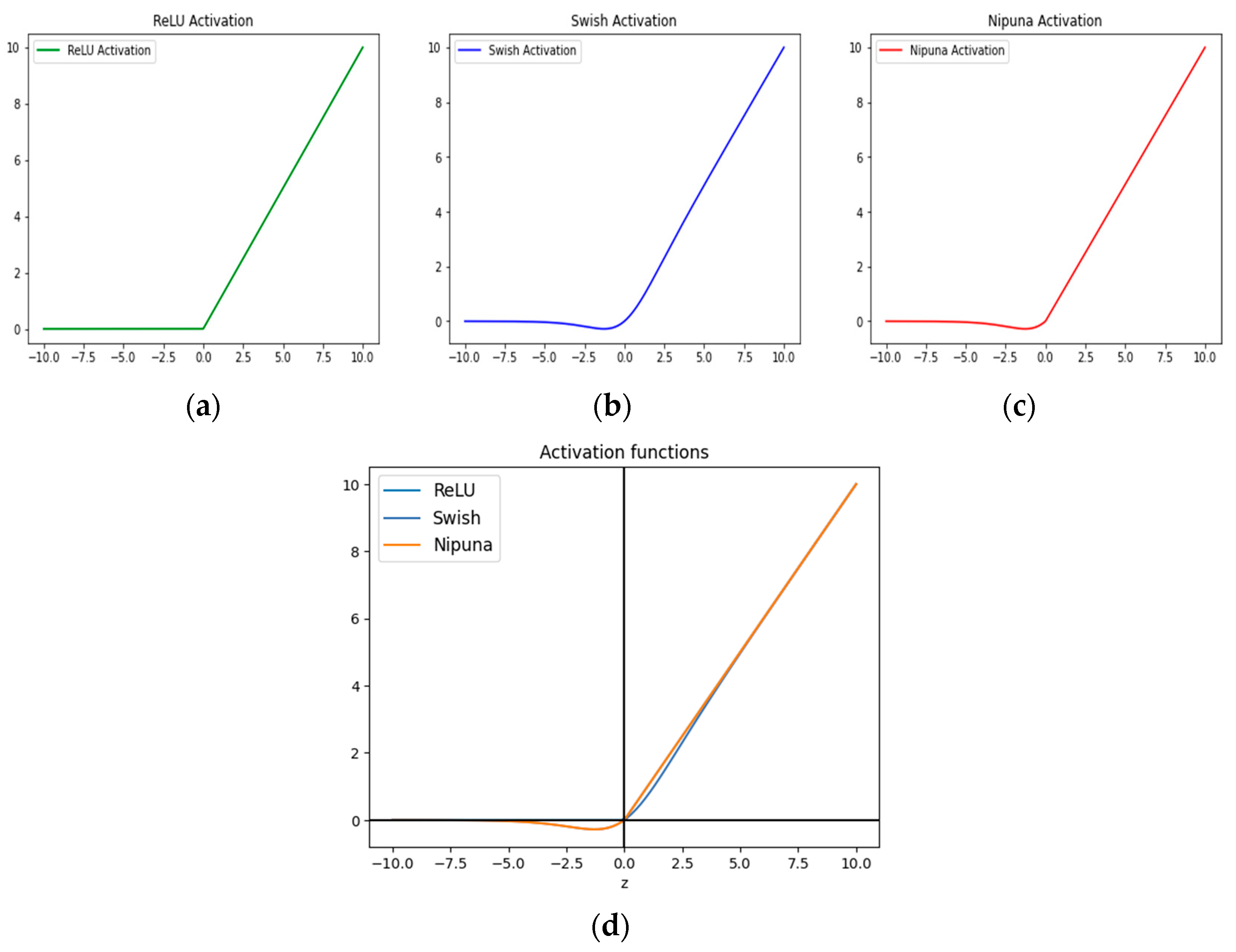
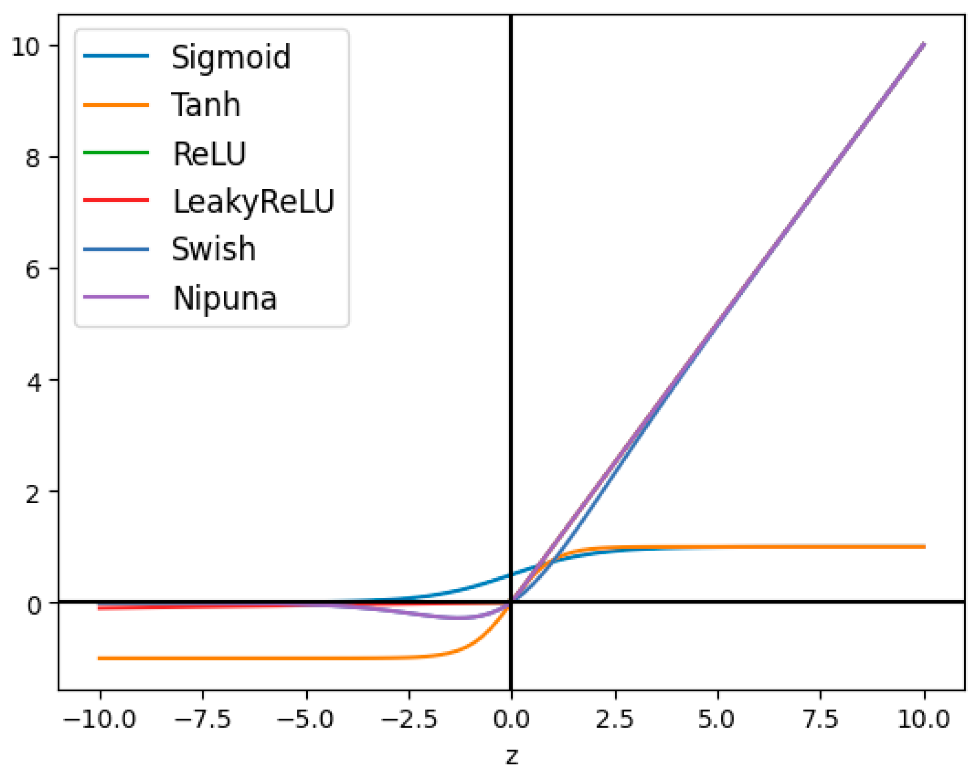
3.1. Proposed Activation Function

Activation functions are typically utilized in neural networks to generate non-linear changes. Taking inspiration from the development of ReLU and Swish, we propose a novel activation function named “NIPUNA” in this study, which is theoretically specified in Equation (7) and has the following universal approximation power of a deep neural network, which helps with the learning of higher-order polynomials for deeper networks:
f ( x ) = max ( g ( x ) , x ) w h e r e   g ( x ) = x ( 1 + e β x )
In Equation (6), the parameter β   value   is   either   a constant or trainable parameter; for this study, we used β   = 1 a trainable parameter.
f ( x ) = d d x ( m a x ( x 1 + e x ) ) = { 1 ,               i f     x e x + 1 0 e x ( x + e x + 1 ) ( e x + 1 ) 2   ,   Otherwise
Figure 1c plots the activation curve of NIPUNA for the value of β = 1 . In Figure 2, we show how the Sigmoid, Tanh, ReLU, Leaky ReLU, Swish and NIPUNA activation works in the network model. They are very similar, but NIPUNA allows the model to capture small negative inputs. Unboundedness above aids training speed, whereas boundness below functions as a regularizes by ignoring inputs spanning from zero to negative infinity.

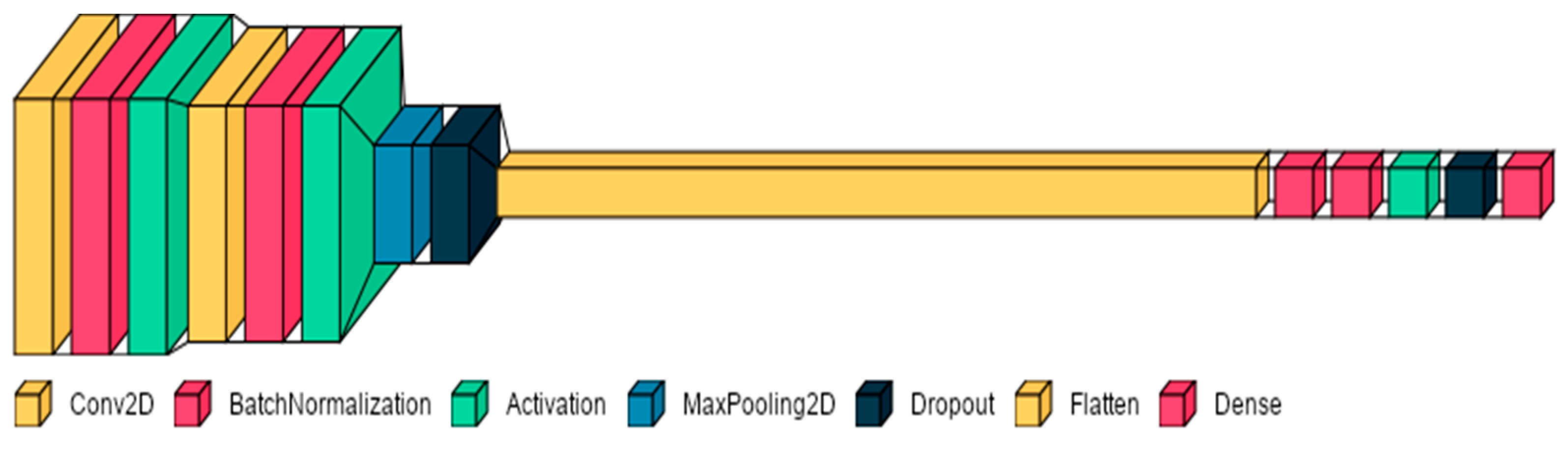
3.2. Customized Convolution Neural Network (CCNN)

We use a customized convolution neural network (CCNN) architecture (shown in Figure 3) to run experiments on the benchmark MINST dataset to test the efficacy of this activation function.
Two convolutional layers and two dense layers are employed in a fourteen-layer CNN. There are 32 kernels in the first convolutional layer and 64 kernels in the fourth convolutional layer. All convolutional layers have the same kernel size (3 × 3). All experiments use the same model architecture and training conditions.

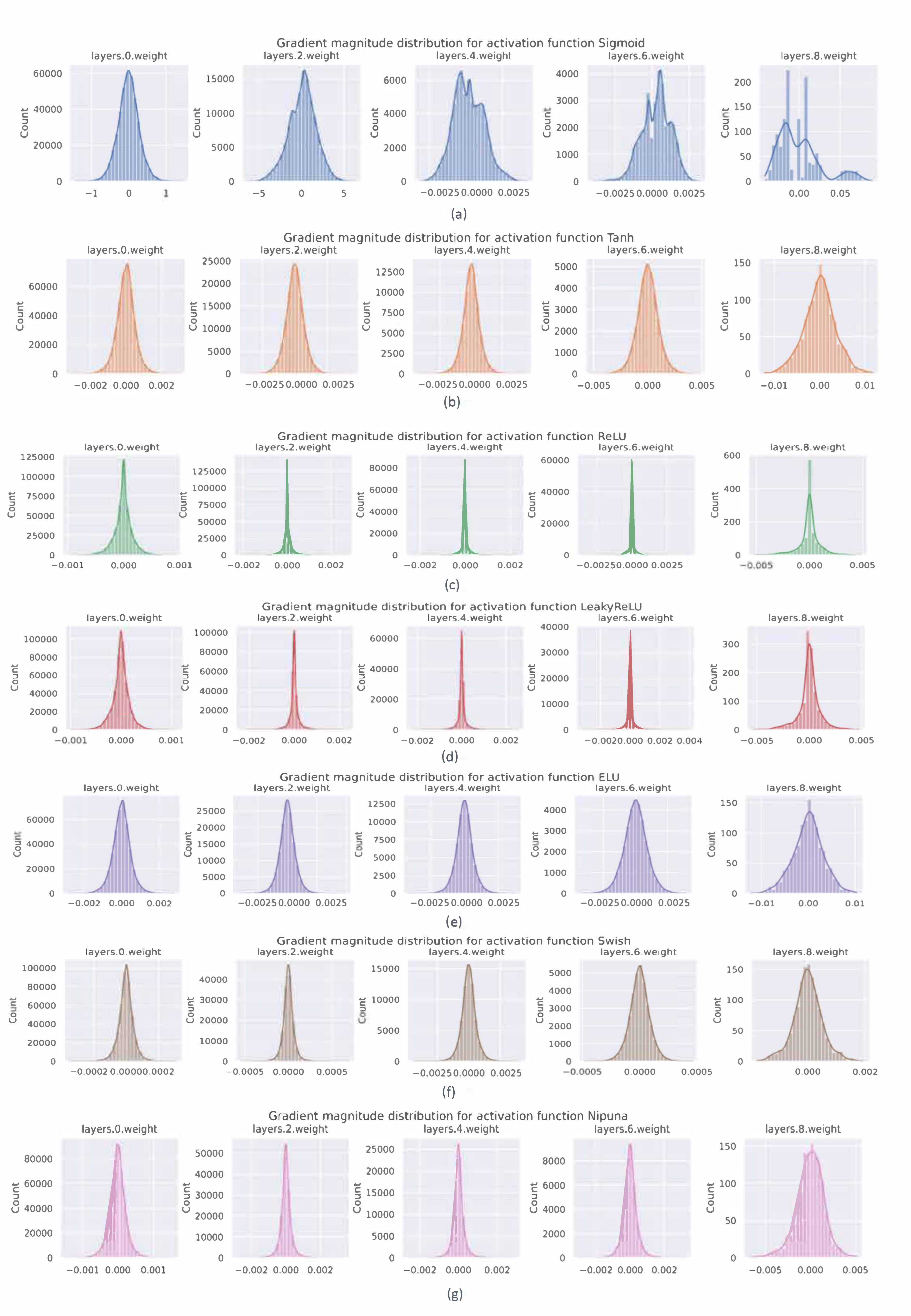
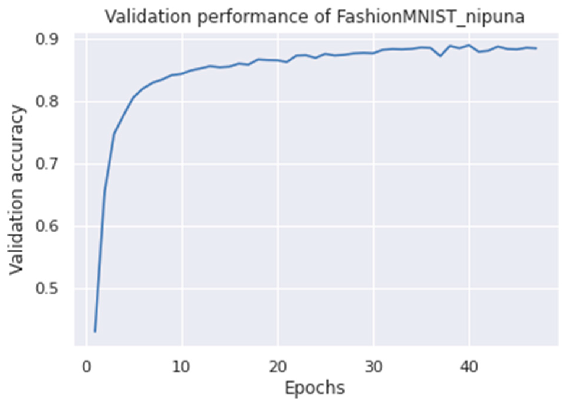
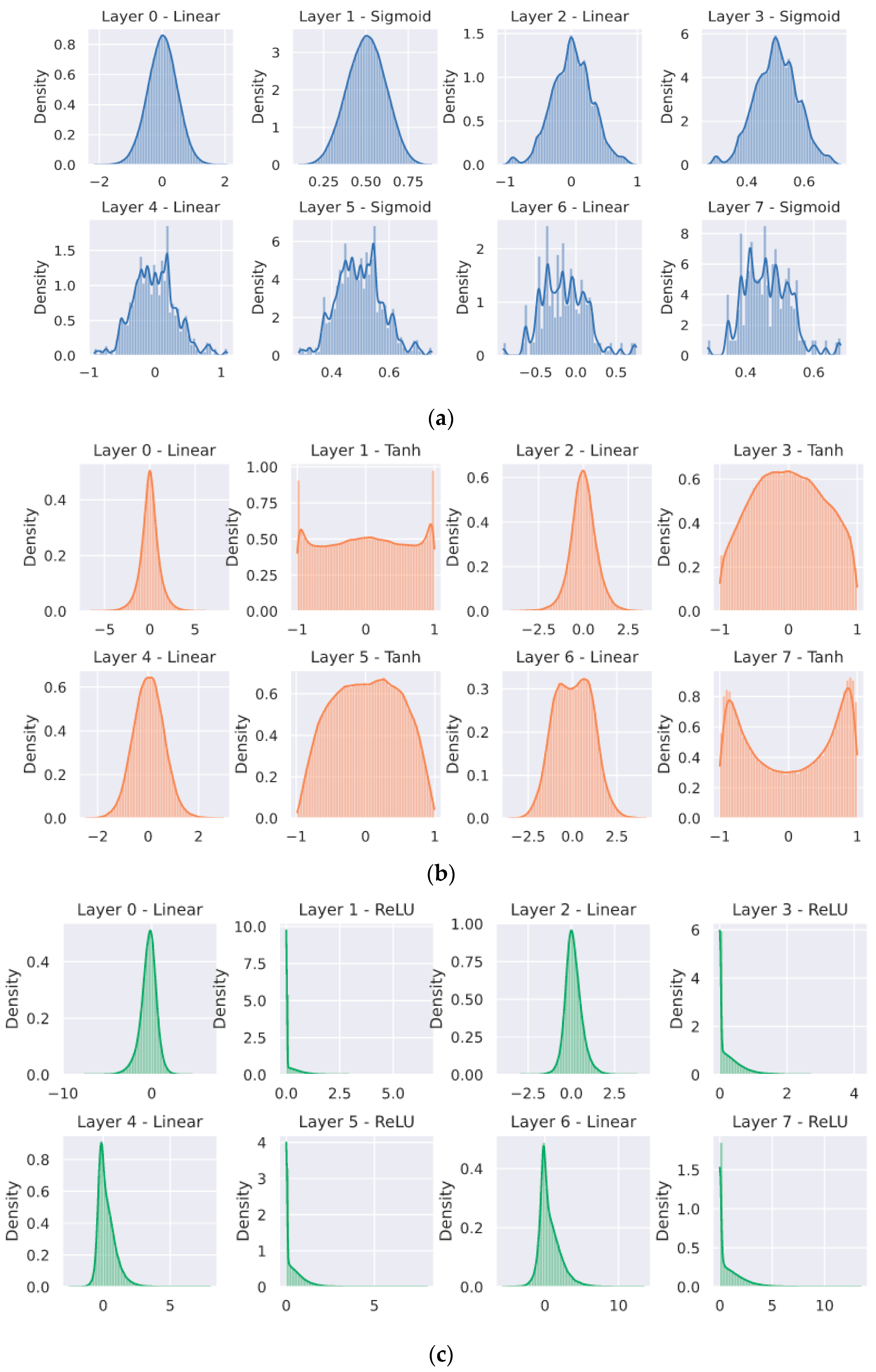
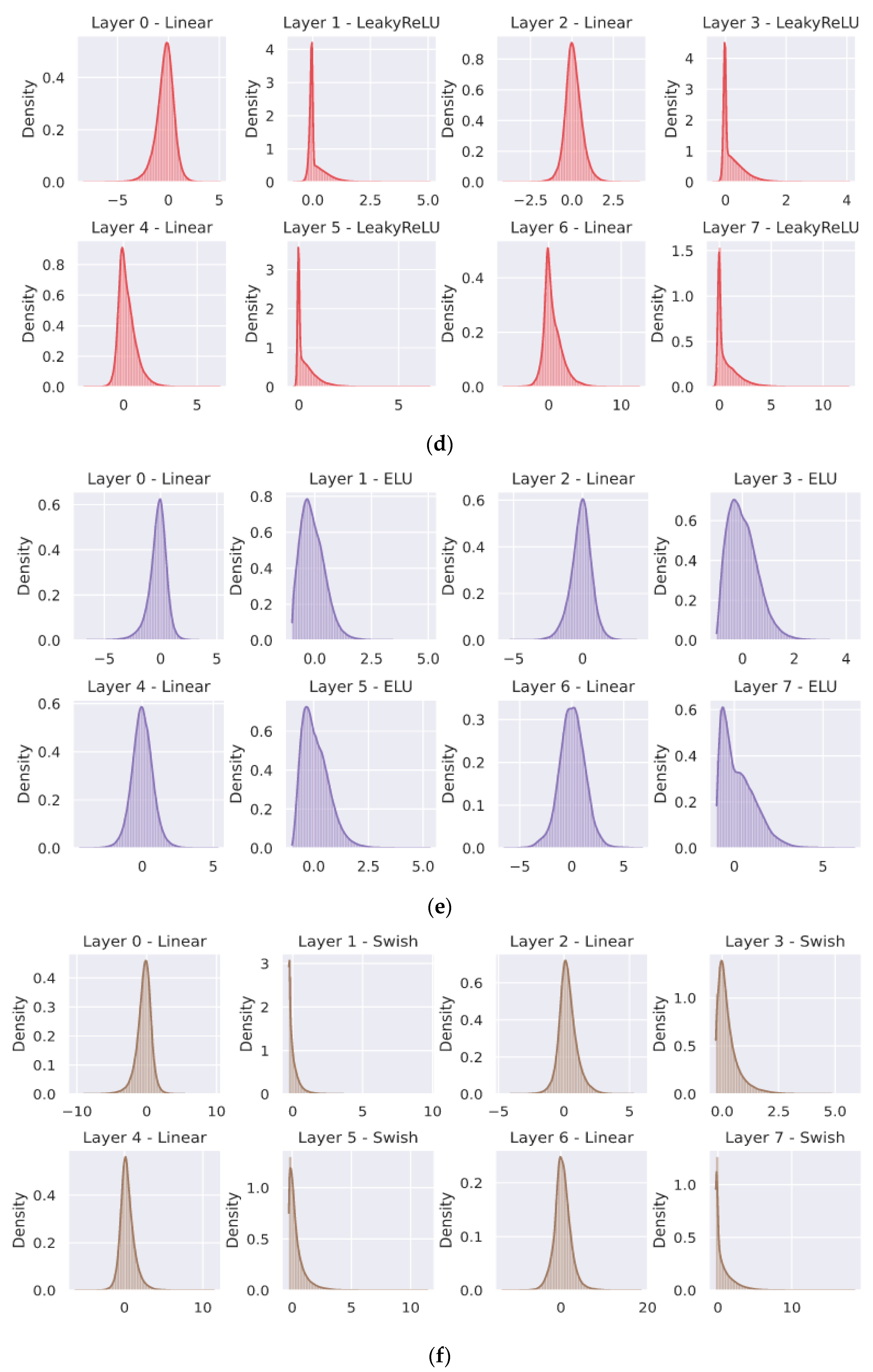
4. Experiments and Their Outcomes

In this section, we determine the proposed activation function’s performance on benchmark datasets: (a) MNIST [28] is a dataset aimed to classify handwritten digits into ten classes; it is a binary image collection of digits with 60,000 training and 10,000 testing samples, and it also comprises ten classes with images that are 28 × 28 in size. In this work, the following state-of-the-art activation functions are compared: Sigmoid [2], Tanh [3], ReLU [6], SELU [12] and Swish [13]. The impacts of the model (NIPUNA) accuracy are depicted in Table 1 and Table 2.
(b) Fashion MNIST [29] is a Zalando article image dataset that consists of black and white clothing photos rather than numbers. A 60,000-sample training set and a 10,000-sample test set, each of which was a 28 × 28 grayscale image labeled with one of ten categories. These samples were used to observe different aspects of the activation functions, such as how they propagate gradients through this network, as well as to test activation performance and gradient flow. We can also study a newly prepared network and see how each activation function affects the gradients by computing the gradients for each network parameter with a batch size of 256 images and then determining how each activation function affects the gradients. Our gradients will vanish until they reach the input layer if the gradient via the activation function is smaller than one. Gradients rise exponentially, and if the activation function’s gradient is greater than one, they may explode. Figure 4a–g shows the gradient magnitude distribution for other popular activation functions.
In Figure 4a, the pattern of the sigmoid activation function is unfavorable. While the output layer seems to have tremendous gradients of up to 0.1, the input layer has the lowest gradient norm at learning rate 1 × 10⁻⁵ and, because of the small maximum gradient of 0.1, the outcome of an adequate learning rate across all layers is not achievable in this circumstance. Across all levels, every one of the activation functions has similar gradient norms. Surprisingly, dead neurons and the zero parts on the left cause a drop in ReLU activation around 0. These functions add different types of adjustable parameters to improve performance to varying extents, and the parameter settings and learning parameters of the activation functions studied in this study are shown in Table 3, along with our model validation performance on the Fashion MNIST dataset, which is shown in Figure 5.
The sigmoid activation function model falls short of outperforming random chance (10 classes => 1/10 for random chance). All other activation functions perform better as well. To arrive at a more accurate conclusion, we model training for multiple seeds and average the results (see Figure 6a–g. A few other factors, however, influence the “optimal” activation function.
Figure 6 illustrates state-of-the-art activation distributions and plots the activation histogram within the network. The activations are less meaningful because the model with sigmoid activation was unable to train adequately, and they all clustered near 0.5. The behavior of the Tanh function is more varied. The activations in the two subsequent layers are closer to zero, even though the input layer has more neurons with activations near −1 and 1, in which the gradients are close to zero. This is most likely the reason that the input layers search the input image for certain traits, which are then merged by the subsequent layers. The activations for the last layer are once again skewed toward the extremes because the classification layer is a weighted average of those values.
Predictably, ReLU exhibits a robust peak at zero. Given that negative values have no gradients, the network has a longer tail toward positive values. The LeakyReLU behaves similarly, whereas the ELU has a more Gaussian distribution. Swish behaves similarly to LeakyReLU, but the activation appears to be in the middle. Although it is worth mentioning that NIPUNA activation employs significantly greater values than other activation functions, it appears to be in the middle (up to 10). Given that all activation functions have slightly different behaviors while achieving identical results for our customized network, it is clear that choosing the “best” activation function depends on a variety of criteria and isn’t the same for all potential networks.

5. Conclusions

A new activation function was proposed in this work (named ‘NIPUNA’). This activation function decomposes into small non-linear segments, each with a distinct activation pattern. It aids in the learning of non-linear transformations for improved feature representation. Our experiments used models and hyperparameters to discuss the effect of the gradient distribution across layers. When these models and hyperparameters are expressly constructed with our activation function (NIPUNA) in mind, we expect even more advantages. Given that the highest gradient provided by Sigmoid is 0.25, it tends to fail in deep neural networks, resulting in vanishing gradients in early layers. This activation function performed equally well or better than Swish in most of the computer vision tasks. In addition, the NIPUNA activation function provided various detailed experiments to demonstrate its superiority. It helps when optimizing the model in terms of convergence to the minimum loss. As a result, the NIPUNA activation function inherits the advantages of ReLU and Swish: (i) it avoids slow training times during near-zero gradients and (ii) it is more computationally efficient when compared with other state-of-the-art activation functions. There are some significant computational costs associated with lightweight deep learning prototypes which will be addressed in future research.

Author Contributions

G.M. proposed the new activation function and experimented. S.K., K.A.A. H.M.Z. and A.W.M. supervised the study, analyzed the results, and provided insightful suggestions for the manuscript. G.M drafted the manuscript. All authors have read and agreed to the published version of the manuscript.

Funding

The research is funded by Researchers Supporting Program at King Saud University, (RSP2023R305).

Data Availability Statement

Not applicable.

Acknowledgments

The authors present their appreciation to King Saud University for funding the publication of this research through Researchers Supporting Program (RSP2023R305), King Saud University, Riyadh, Saudi Arabia.

Conflicts of Interest

The authors declare no conflict of interest.

References

  1. Goodfellow, I.; Bengio, Y.; Courville, A. Deep Learning; MIT Press: Cambridge, UK, 2016. [Google Scholar]
  2. Yamada, T.; Yabuta, T. Neural network controller using autotuning method for nonlinear functions. IEEE Trans. Neural Netw. 1992, 3, 595–601. [Google Scholar] [CrossRef] [PubMed]
  3. Chen, C.T.; Chang, W.D. A feedforward neural network with function shape autotuning. Neural Netw. 1996, 9, 627–641. [Google Scholar] [CrossRef]
  4. Hahnloser, R.H.; Sarpeshkar, R.; Mahowald, M.A.; Douglas, R.J.; Seung, H.S. Digital selection and analogue amplification coexist in a cortex-inspired silicon circuit. Nature 2000, 405, 947–951. [Google Scholar] [CrossRef] [PubMed]
  5. Jarrett, K.; Kavukcuoglu, K.; Ranzato, A.; Le Cun, Y. What is the best multi-stage architecture for object recognition? In Proceedings of the 2009 IEEE 12th International Conference on Computer Vision, Kyoto, Japan, 29 September–2 October 2009; pp. 2146–2153. [Google Scholar]
  6. Nair, V.; Hinton, G.E. Rectified linear units improve restricted Boltzmann machines. In Proceedings of the 27th International Conference on Machine Learning (ICML-10), Haifa, Israel, 21–24 June 2010; pp. 807–814. [Google Scholar]
  7. Richard, H.R.; Hahnloser, H.; Seung, S. Permitted and forbidden sets in symmetric threshold-linear networks. In Advances in Neural Information Processing Systems; MIT Press: Cambridge, UK, 2001; pp. 217–223. [Google Scholar]
  8. Hinton, G.; Salakhutdinov, R. An efficient learning procedure for deep Boltzmann machines. Neural Comput. 2012, 24, 1967–2006. [Google Scholar]
  9. Maas, A.L.; Hannun, A.Y.; Ng, A.Y. Rectifier nonlinearities improve neural network acoustic models. In Proceedings of the 30th International Conference on Machine Learning, Atlanta, GA, USA, 17–19 June 2013; Volume 30, p. 3. [Google Scholar]
  10. He, K.; Zhang, X.; Ren, S.; Sun, J. Delving deep into rectifiers: Surpassing human-level performance on imagenet classification. In Proceedings of the IEEE International Conference on Computer Vision, Santiago, Chile, 7–13 December 2015; pp. 1026–1034. [Google Scholar]
  11. Clevert, D.A.; Unterthiner, T.; Hochreiter, S. Fast and accurate deep network learning by exponential linear units (elus). arXiv 2015, arXiv:1511.07289. [Google Scholar]
  12. Günter, K.; Unterthiner, T.; Mayr, A.; Hochreiter, S. Self-normalizing neural networks. In Proceedings of the 31st International Conference on Neural Information Processing Systems, Long Beach, CA, USA, 4–9 December 2017; pp. 972–981. [Google Scholar]
  13. Prajit, R.; Zoph, B.; Le, Q.V. Swish: A self-gated activation function. arXiv 2017, arXiv:1710.05941. [Google Scholar]
  14. Singh, B.V.; Kumar, V. Linearized sigmoidal activation: A novel activation function with tractable non-linear characteristics to boost representation capability. Expert Syst. Appl. 2019, 120, 346–356. [Google Scholar]
  15. Lohani, H.K.; Dhanalakshmi, S.; Hemalatha, V. Performance Analysis of Extreme Learning Machine Variants with Varying Intermediate Nodes and Different Activation Functions. In Cognitive Informatics and Soft Computing; Springer: Berlin/Heidelberg, Germany, 2019; pp. 613–623. [Google Scholar]
  16. Krizhevsky, A.; Sutskever, I.; Hinton, G.E. Imagenet classification with deep convolutional neural networks. In Proceedings of the Advances in Neural Information Processing Systems, Lake Tahoe, Nevada, 3–6 December 2012; Volume 1, pp. 1097–1105. [Google Scholar]
  17. Njikam, S.; Nasser, A.; Zhao, H. A novel activation function for multilayer feed-forward neural networks. Appl. Intell. 2016, 45, 75–82. [Google Scholar] [CrossRef]
  18. Xu, B.; Wang, N.; Chen, T.; Li, M. Empirical evaluation of rectified activations in convolutional network. arXiv 2015, arXiv:1505.00853. [Google Scholar]
  19. Hendrycks, D.; Gimpel, K. Gaussian error linear units (gelus). arXiv 2016, arXiv:1606.08415. [Google Scholar]
  20. Trottier, L.; Giguere, P.; Chaib-Draa, B. Parametric exponential linear unit for deep convolutional neural networks. In Proceedings of the 16th IEEE International Conference on Machine Learning and Applications (ICMLA), Cancun, Mexico, 18–21 December 2017; pp. 207–214. [Google Scholar]
  21. Faruk, E.Ö. A novel type of activation function in artificial neural networks: Trained activation function. Neural Netw. 2018, 99, 148–157. [Google Scholar]
  22. Diganta, M. Mish: A self-regularized non-monotonic neural activation function. arXiv 2019, arXiv:1908.08681. [Google Scholar]
  23. Liu, X.; Di, X. TanhExp: A smooth activation function with high convergence speed for lightweight neural networks. IET Computer Vision 2021, 15, 136–150. [Google Scholar] [CrossRef]
  24. Sayan, N.; Bhattacharyya, M.; Mukherjee, A.; Kundu, R. SERF: Towards better training of deep neural networks using log-Softplus ERror activation Function. In Proceedings of the IEEE/CVF Winter Conference on Applications of Computer Vision, Waikoloa, HI, USA, 3–7 January 2023; pp. 5324–5333. [Google Scholar]
  25. Wang, X.; Ren, H.; Wang, A. Smish: A Novel Activation Function for Deep Learning Methods. Electronics 2022, 11, 540. [Google Scholar] [CrossRef]
  26. Shen, S.L.; Zhang, N.; Zhou, A.; Yin, Z.Y. Enhancement of neural networks with an alternative activation function tanhLU. Expert Syst. Appl. 2022, 199, 117181. [Google Scholar] [CrossRef]
  27. Vallés-Pérez, I.; Soria-Olivas, E.; Martínez-Sober, M.; Serrano-López, A.J.; Vila-Francés, J.; Gómez-Sanchís, J. Empirical study of the modulus as activation function in computer vision applications. Eng. Appl. Artif. Intell. 2023, 120, 105863. [Google Scholar] [CrossRef]
  28. Deng, L. The MNIST database of handwritten digit images for machine learning research. IEEE Signal Process. Mag. 2012, 29, 141–142. [Google Scholar] [CrossRef]
  29. Han, X.; Rasul, K.; Vollgraf, R. Fashion-MNIST: A novel image dataset for benchmarking machine learning algorithms. arXiv 2017, arXiv:1708.07747. [Google Scholar]
Figure 1. Illustration of activation functions: (a) Rectified Linear Unit (ReLU) Ref. [6], (b) Swish activation function (SWISH) Ref. [13], (c) NIPUNA activation function, (d) three graphical representations of activation functions.
Axioms 12 00246 g001
Figure 2. Commonly used baseline activation functions.
Axioms 12 00246 g002
Figure 3. Customized convolutional neural network.
Axioms 12 00246 g003
Figure 4. This is a figure showing the gradient magnitude distribution for other state-of-the-art activation functions. (a) Illustration of gradient magnitude of the Sigmoid activation function; (b) illustration of gradient magnitude of the tanh activation function; (c) illustration of gradient magnitude of the ReLU activation function; (d) illustration of gradient magnitude of the LeakyReLU activation function; (e) illustration of gradient magnitude of the ELU activation function; (f) illustration of gradient magnitude of the Swish activation function; (g) illustration of gradient magnitude of the NIPUNA activation function.
Axioms 12 00246 g004
Figure 5. Validation performance of proposed activation function on the Fashion MNIST dataset.
Axioms 12 00246 g005
Figure 6. This is a figure showing the activation distribution for other state-of-the-art activation functions. (a). Layer-wise activation distribution for the sigmoid activation function; (b) layer-wise activation distribution for the tanh activation function; (c) layer-wise activation distribution for the ReLU activation function; (d) layer-wise activation distribution for the LeakyReLU activation function; (e) layer-wise activation distribution for the ELU activation function; (f) layer-wise activation distribution for the Swish activation function; (g) layer-wise activation distribution for the NIPUNA activation function.
Axioms 12 00246 g006aAxioms 12 00246 g006bAxioms 12 00246 g006c
Table 1. Compares the proposed activation function’s classification accuracies (for 50 Epochs).
Dataset: MNIST (50 Epochs), Optimizer = Adam, Kernel_Initializer = HeNormal
Customized
CNN
Activation TypeAccuracy Loss
TestTrainTestTrain
Sigmoid0.93720.96910.24040.1243
Tanh0.92500.97900.29300.0809
ReLU0.93660.98390.26840.0859
SELU0.92470.96120.25900.1321
Swish0.93110.98500.29600.0739
NIPUNA (Proposed)0.93410.98740.26520.0723
Table 2. Compares the proposed activation function’s classification accuracies (for 100 Epochs).
Dataset: MNIST (100 Epochs), Optimizer = SGD, Kernel_Initializer = HeNormal
Customized
CNN
Activation TypeAccuracy Loss
TestTrainTestTrain
Sigmoid0.92420.95110.32570.1579
Tanh0.91500.96200.39300.1274
ReLU0.92660.93490.21140.1810
SELU0.93070.97230.31040.1620
Swish0.92360.95140.22160.1356
NIPUNA (Proposed)0.93370.99690.36010.0212
Table 3. A summary of the activation functions studied in this study.
Activation FunctionParameters Setting/InitializationLearned Parameters
Sigmoid----
Tanh----
ReLU----
SELUλ ≈ 1.0507, α ≈ 1.6732 α ,   λ
Swish β = 0 ,   1 ,   0.5 , σ = 0.1 β , σ
NIPUNA β = 1 β
Disclaimer/Publisher’s Note: The statements, opinions and data contained in all publications are solely those of the individual author(s) and contributor(s) and not of MDPI and/or the editor(s). MDPI and/or the editor(s) disclaim responsibility for any injury to people or property resulting from any ideas, methods, instructions or products referred to in the content.

