Composition and Decomposition of Positive Linear Operators (VIII)

Abstract

In a series of papers, most of them authored or co-authored by H. Gonska, several authors investigated problems concerning the composition and decomposition of positive linear operators defined on spaces of functions. For example, given two operators with known properties, A and B, we can find the properties of the composed operator $A\circ B$, such as the eigenstructure, the inverse, the Voronovskaja formula, and the second-order central moments. One motivation for studying composed operators is the possibility to obtain better rates of approximation and better Voronovskaja formulas. Our paper will address such problems involving compositions of some classical positive linear operators. We present general results as well as numerical experiments.

1. Introduction

The composition and decomposition of positive linear operators were investigated in a series of papers [1,2,3]. The considerable subjects of the studies were:

(i)

The transfer of the properties of the operators to be composed to the resulting operator;

(ii)

The possibility to represent a given operator in a nontrivial way as a composition of two operators.

Related to the decomposition of a positive linear operator, the inverses of operators are important ingredients (see [1,4,5]). Their important role is motivated in particular by the problem of a possible decomposition of the Bernstein classical operator into two nontrivial factors as positive linear operators (see [2]). Voronovskaja-type results for inverses of operators acting on polynomials were obtained in [4,5]. In these kinds of problems, the eigenstructures of the operators and their inverses are useful tools (see [4]).

Usually, the sequences of classical positive linear operators are convergent toward the identity operator. However, special attention was also paid to sequences convergent to an operator different from the identity. This approach was used in [6] with probabilistic methods. In [7], results of this type were obtained with analytic methods.

This paper is devoted to similar problems for certain integral positive linear operators.

Consider the Rathore operator

$$W_{n}f\left(x\right)={\displaystyle \frac{n^{nx}}{\Gamma \left(nx\right)}}{\int }_0^{\infty }{e}^{-nt}{t}^{nx-1}f\left(t\right)dt,$$

and the Gamma operator

$$G_{n}f\left(x\right)={\displaystyle \frac{{\left(nx\right)}^{n+1}}{n!}}{\int }_0^{\infty }{\displaystyle \frac{1}{s^{n+2}}}{e}^{-\frac{nx}{s}}f\left(s\right)ds.$$

They are well known and widely studied in the literature. We will be interested in the composition of these two integral positive linear operators, which is a new integral positive linear operator denoted by

$${\mathcal{F}}_n:=W_n\circ G_n.$$

Its explicit expression can be seen in formula (1) below.

The eigenstructure of a positive linear operator is extremely useful in Approximation Theory. There is a long list of papers investigating the eigenstructure and its consequences concerning the approximation properties of the corresponding family of positive linear operators.

Section 2 is devoted to the eigenstructure of ${\mathcal{F}}_n$. We give explicit expressions of the eigenvalues and the eigenfunctions for ${\mathcal{F}}_n$ restricted to polynomials. We mention the relationship between these eigenpolynomials and those of the classical Bernstein operators described in [8]. A typical problem in studying a sequence of discrete or integral positive linear operators is that of determining its Voronovskaja formula. As it is well known, this is related with the determination of the saturation class of the respective sequence. The Voronovskaja limit gives us indications concerning the quality of approximation furnished by the sequence.

In Section 3, we recall a general result from [9] and apply it in order to establish the Voronovskaja-type formula for the sequence ${\left({\mathcal{F}}_n\right)}_{n\ge 1}$. A similar result for the sequence ${\left({\mathcal{F}}_n^{-1}\right)}_{n\ge 1}$ is established using the eigenstructure of ${\mathcal{F}}_n$.

Probabilistic methods are very useful in constructing positive linear operators and in studying their properties. A specific application of such methods can be found in [6] (see also [7] and the references therein). More precisely, it consists of modifying a given sequence, which converges to the identity operator in order to obtain a new sequence with limit different from the identity.

Section 4 is devoted to the convergence of a special modification of the sequence ${\left({\mathcal{F}}_n\right)}_{n\ge 1}$ in the spirit of the papers [6,7].

Central objects of study in Approximation Theory by positive linear operators are the moments (the images of the monomials) and the central moments. They are related with the Voronovskaja formulas and the rates of convergence of the involved sequences.

Voronovskaja-type formulas and the second-order central moments for the composition of some classical operators are investigated in Section 5.

Section 6 is devoted to conclusions and further work.

The involved operators are defined on functions for which the integrals and series are convergent.

2. The Eigenstructure of ${\mathcal{F}}_{\mathit{n}}$

In this section, we give explicit expressions of the eigenvalues and the eigenfunctions for ${\mathcal{F}}_n$ restricted to polynomials. The eigenstructure of ${\mathcal{F}}_n$ obtained by us in this paper is related to the eigenstructures of other operators (see, e.g., [8]).

The explicit form of the operator ${\mathcal{F}}_n$ is in [10]

$${\mathcal{F}}_{n}f\left(x\right)={\displaystyle \frac{{\left(nx\right)}_{n+1}}{n!}}{\int }_0^{\infty }{\displaystyle \frac{t^{nx-1}}{{(1+t)}^{n+nx+1}}}f\left(t\right)dt.$$

(1)

Consider the monomials denoted by $e_j\left(t\right)=t^j$, $t\ge 0$, $j=0,1,\cdots$ By a direct calculation one finds (see also [10]) that

$${\mathcal{F}}_n{e}_j\left(x\right)={\displaystyle \frac{{\left(nx\right)}_j}{{(n-j+1)}_j}},n\ge j,$$

(2)

where ${\left(a\right)}_j$ denotes the raising factorial, that is ${\left(a\right)}_j=a(a+1)\cdots (a+j-1)$, for $j\ge 1$ and ${\left(a\right)}_0=1$.

Let ${\Pi }_n$ be the space of polynomial functions of the highest degree at n. From (2), it follows that the eigenvalues of the operator ${\mathcal{F}}_n:{\Pi }_n\to {\Pi }_n$ are the numbers

$$\begin{array}{cc}\hfill & {\nu }_k^{\left(n\right)}={\displaystyle \frac{n^k}{{(n-k+1)}_k}},0\le k\le n.\hfill \end{array}$$

(3)

Let

$${\displaystyle r_k^{\left(n\right)}\left(x\right):=\sum _{j=0}^{k}b(n,k,j)x^j,}$$

(4)

be the associated monic eigenpolynomials. This means that

$${\mathcal{F}}_n{r}_k^{\left(n\right)}={\nu }_k^{\left(n\right)}{r}_k^{\left(n\right)},k=0,\cdots ,n,$$

(5)

and the coefficient of the dominant power of x in the polynomial $r_k^{\left(n\right)}$ is equal to 1.

In particular, $r_0^{\left(n\right)}=e_0$ and $r_1^{\left(n\right)}=e_1$, and consequently we deduce that

$$b(n,0,0)=1,b(n,1,0)=0,b(n,1,1)=1.$$

(6)

From (2) and (4), it follows that

$${\displaystyle {\mathcal{F}}_n{r}_k^{\left(n\right)}\left(x\right)=\sum _{i=0}^{k}b(n,k,i){\displaystyle \frac{{\left(nx\right)}_i}{{(n-i+1)}_i}}={\displaystyle \frac{n^k}{{(n-k+1)}_k}}\sum _{i=0}^{k}b(n,k,i)x^i.}$$

(7)

From the definition of Stirling numbers of the first kind $s(j,i)$, we obtain

$${\displaystyle {\left(nx\right)}_j=\sum _{i=0}^{j}s(j,i){(-1)}^{j-i}{n}^i{x}^i,}$$

(8)

Combining the formulas (7) and (8) we obtain

$${\displaystyle \sum _{i=0}^k\sum _{j=i}^k{\displaystyle \frac{b(n,k,j)s(j,i){(-1)}^{j-i}{n}^i}{{(n-j+1)}_j}}{x}^i=\sum _{i=0}^k{\displaystyle \frac{b(n,k,i)n^k}{{(n-k+1)}_k}}{x}^i,}$$

and therefore

$$\sum _{j=i}^k{\displaystyle \frac{b(n,k,j)s(j,i){(-1)}^{j-i}}{{(n-j+1)}_j}}={\displaystyle \frac{b(n,k,i)n^{k-i}}{{(n-k+1)}_k}},i=0,\cdots ,k.$$

This can be written as

$${\displaystyle \frac{b(n,k,i)}{{(n-i+1)}_i}}+\sum _{j=i+1}^k{\displaystyle \frac{b(n,k,j)s(j,i){(-1)}^{j-i}}{{(n-j+1)}_j}}={\displaystyle \frac{b(n,k,i)n^{k-i}}{{(n-k+1)}_k}},i=0,\cdots ,k.$$

A direct calculation allows us to solve this system for $b(n,k,i)$ and, consequently, we obtain

$$b(n,k,i)={\displaystyle \frac{{\sum }_{j=i+1}^k{(-1)}^{j-i-1}s(j,i){(n-k+1)}_{k-j}b(n,k,j)}{{(n-k+1)}_{k-i}-n^{k-i}}},i=k-1,k-2,\cdots ,0.$$

(9)

Since $r_k^{\left(n\right)}$ is a monic polynomial, we have

$$b(n,k,k)=1.$$

(10)

From (9) and (10), we can recurrently determine the coefficients $b(n,k,i)$, $i=k-1,$$k-2,$$\cdots ,0.$

In particular, we find that

$$\begin{array}{cc}& b(n,k,k-1)={\displaystyle \frac{k}{2}},\hfill \\ \hfill & b(n,k,k-2)={\displaystyle \frac{k(k-1)(k-2)}{24}}{\displaystyle \frac{6n-3k+5}{(2k-3)n-(k-1)(k-2)}}.\hfill \end{array}$$

In the sequel, we use the following notation

$${\displaystyle b^{*}(k,j)=\underset{n\to \infty }{lim}b(n,k,j),j=0,\cdots ,k.}$$

From (6), we deduce immediately that

$$b^{*}(0,0)=1,b^{*}(1,0)=0,b^{*}(1,1)=1.$$

Moreover, (10) leads to the relation

$$b^{*}(k,k)=1.$$

(11)

Lemma 1. 

Let $k\ge 2$ and $j=0\cdots ,k$ be integers. Then, one has

$$b^{*}(k,j)={(-1)}^{k-j}\prod _{l=1}^{k-j}{\displaystyle \frac{(k-l+1)(k-l)}{l(l-2k+1)}}.$$

(12)

Proof. 

We prove the relation (12) by induction with respect to j. It is true for $j=k$ according to (11). Suppose that it is true for all $j\ge i+1$ and let us prove it for $j=i$.

By a small manipulation, Formula (9) can be written under the form

$$\begin{array}{cc}\hfill b(n,k,i)& ={\displaystyle \frac{s(i+1,i){(n-k+1)}_{k-i-1}b(n,k,i+1)}{{(n-k+1)}_{k-i}-n^{k-i}}}\hfill \\ \hfill & +{\displaystyle \frac{{\sum }_{j=i+2}^k{(-1)}^{j-i-1}s(j,i){(n-k+1)}_{k-j}b(n,k,j)}{{(n-k+1)}_{k-i}-n^{k-i}}}.\hfill \end{array}$$

Passing the limit when n goes to infinity, after some elementary calculations, we obtain

$$b^{*}(k,i)={\displaystyle \frac{i(i+1)}{(k-i)(k+i-1)}}{b}^{*}(k,i+1).$$

Consequently, using (12) for $j=i+1$, it follows that

$$\begin{array}{cc}\hfill b^{*}(k,i)& ={\displaystyle \frac{i(i+1)}{(k-i)(k+i-1)}}·{(-1)}^{k-i-1}{\displaystyle \prod _{l=1}^{k-i-1}}{\displaystyle \frac{(k-l+1)(k-l)}{l(l-2k+1)}}\hfill \\ \hfill & ={(-1)}^{k-i}{\displaystyle \prod _{l=1}^{k-i}}{\displaystyle \frac{(k-l+1)(k-l)}{l(l-2k+1)}},\hfill \end{array}$$

(13)

and so the proof by induction is complete. □

Remark 1. 

Using (4), we obtain

$${\displaystyle r_k^{*}\left(x\right):=\underset{n\to \infty }{lim}{r}_k^{\left(n\right)}\left(x\right)=\sum _{i=0}^k{b}^{*}(k,i)x^i=\sum _{i=0}^k{(-1)}^{k-i}{c}^{*}(i,k)x^i,}$$

(14)

where $c^{*}(i,k)$ are the coefficients from [8] (Th. 4.1). More precisely,

$$\sum _{i=0}^k{c}^{*}(i,k)x^i=p_k^{*}\left(x\right),k\ge 0,$$

where $p_0^{*}\left(x\right)=1$, $p_1^{*}\left(x\right)=x-\frac{1}{2}$ and for $k\ge 2$,

$$p_k^{*}\left(x\right)={\displaystyle \frac{k!(k-2)!}{(2k-2)!}}x(x-1)P_{k-2}^{(1,1)}(2x-1).$$

Here, $P_m^{(1,1)}$ are the Jacobi polynomials, which are orthogonal with respect to the weight $(1-t)(1+t)$ on the interval $[-1,1]$.

3. Voronovskaja-Type Results

First, we recall a general result from [9] involving positive linear operators. Using it, we establish the Voronovskaja-type formula for the sequence ${\left({\mathcal{F}}_n\right)}_{n\ge 1}$. Generally, the inverse of a positive linear operator is not necessarily positive. So, to establish the Voronovskaja-type formula for the sequence ${\left({\mathcal{F}}_n^{-1}\right)}_{n\ge 1}$ acting on polynomial functions, we use the eigenstructure of ${\mathcal{F}}_n^{-1}$ deduced from the eigenstructure of ${\mathcal{F}}_n$, which was established in Section 2 of this paper.

Let $\phi \in C^2[0,\infty )$, $\phi \left(0\right)=0$, ${\phi }^{\prime }\left(t\right)>0$, $t\in (0,\infty )$, ${\displaystyle \underset{t\to \infty }{lim}\phi \left(t\right)=\infty }$. Consider the space of functions

$$E_{\phi }:=\left\{f\in C[0,\infty )\left|{\displaystyle \underset{t\ge 0}{sup}{\displaystyle \frac{\left|f\right(t\left)\right|}{1+{\phi }^2\left(t\right)}}<\infty }\right.\right\}$$

endowed with the norm ${\displaystyle {\parallel f\parallel }_{\phi }:=\underset{t\ge 0}{sup}{\displaystyle \frac{\left|f\right(t\left)\right|}{1+{\phi }^2\left(t\right)}}}$, $f\in E_{\phi }$.

Theorem 1 

([9]). Let $x>0$ be given, and let ${\Psi }_x\left(t\right):=\phi \left(t\right)-\phi \left(x\right)$, $t\ge 0$. Denote by $E_{\phi }^x$ a linear subspace of $C[0,\infty )$, such that $E_{\phi }\subset E_{\phi }^x$ and ${\Psi }_x^4\in E_{\phi }^x$. Let $L_n:E_{\phi }^x\to C[0,\infty )$ be a sequence of positive linear operators, such that

(i) 

${\displaystyle \underset{n\to \infty }{lim}n\left(L_n{e}_0\left(x\right)-1\right)=0}$,

(ii) 

${\displaystyle \underset{n\to \infty }{lim}n{L}_n{\Psi }_x\left(x\right)=b\left(x\right)}$,

(iii) 

${\displaystyle \underset{n\to \infty }{lim}n{L}_n{\Psi }_x^2\left(x\right)=2a\left(x\right)}$,

(iv) 

${\displaystyle \underset{n\to \infty }{lim}n{L}_n{\Psi }_x^4\left(x\right)=0}$.

If $f\in E_{\phi }$ and there exists $f^{″}\left(x\right)\in \mathbb{R}$, then

$${\displaystyle \underset{n\to \infty }{lim}n\left(L_{n}f\left(x\right)-f\left(x\right)\right)={\displaystyle \frac{a\left(x\right)}{{\phi }^{\prime }{\left(x\right)}^2}}{f}^{″}\left(x\right)+{\displaystyle \frac{b\left(x\right){\phi }^{\prime }{\left(x\right)}^2-a\left(x\right){\phi }^{″}\left(x\right)}{{\phi }^{\prime }{\left(x\right)}^3}}{f}^{\prime }\left(x\right).}$$

(15)

For similar results in related contexts see [11,12].

We apply Theorem 1 for the sequence ${\left(\mathcal{F}\right)}_{n\ge 1}$, choosing the function $\phi \left(t\right)=t$. To this end, we need the following identities, which can be established by elementary calculation

$$\begin{array}{cc}\hfill & {\mathcal{F}}_n{e}_0\left(x\right)=1,{\mathcal{F}}_n{\Psi }_x\left(x\right)=0,\hfill \\ \hfill & {\mathcal{F}}_n{\Psi }_x^2\left(x\right)={\displaystyle \frac{x(x+1)}{n-1}},\hfill \\ \hfill & {\mathcal{F}}_n{\Psi }_x^4\left(x\right)={\displaystyle \frac{3x(x+1)(n{x}^2+nx+6^2+6x+2)}{(n-3)(n-2)(n-1)}}.\hfill \end{array}$$

It follows immediately that conditions (i)–(iv) are fulfilled with $b\left(x\right)=0$ and $a\left(x\right)={\displaystyle \frac{x(x+1)}{2}}$. So, we have proved the following Voronovskaja-type result.

Theorem 2. 

Let $\phi \left(t\right)=t$, $t\ge 0$ and $f\in E_{\phi }$, and suppose that there exists $f^{″}\left(x\right)\in \mathbb{R}$. Then,

$${\displaystyle \underset{n\to \infty }{lim}n\left({\mathcal{F}}_{n}f\left(x\right)-f\left(x\right)\right)={\displaystyle \frac{x(x+1)}{2}}{f}^{″}\left(x\right).}$$

In the sequel, we consider the restriction ${\mathcal{F}}_n:{\Pi }_n\to {\Pi }_n$, which is bijective because all the eigenvalues ${\nu }_k^{\left(n\right)},k=0,\cdots ,n$ are different from 0. We will establish a Voronovskaja-type result for ${\mathcal{F}}_n^{-1}:{\Pi }_n\to {\Pi }_n$. Theorem 1 is not applicable because the operators ${\mathcal{F}}_n^{-1}$ are not positive. This can be seen from the relation ${\mathcal{F}}_n^{-1}{e}_2\left(x\right)={\displaystyle \frac{1}{n}}x\left((n-1)x-1\right)$, which shows that ${\mathcal{F}}_n^{-1}{e}_2\left(x\right)$ is negative for $0<1<{\displaystyle \frac{1}{n-1}}$.

Our main tool in establishing a Voronovskaja-type formula for the sequence $\left({\mathcal{F}}_n^{-1}\right)$ will be the previously described eigenstructure of the operator ${\mathcal{F}}_n$.

Theorem 3. 

Let $m\ge 1$, $p\in {\Pi }_m$, and $x\ge 0$ be given. Then,

$${\displaystyle \underset{n\to \infty }{lim}n({\mathcal{F}}_n^{-1}p\left(x\right)-p\left(x\right))=-{\displaystyle \frac{x(x+1)}{2}}{p}^{″}\left(x\right).}$$

(16)

Proof. 

Let $n\ge m$. Then, $\{r_0^{\left(n\right)}\left(x\right),r_1^{\left(n\right)}\left(x\right),\cdots ,r_m^{\left(n\right)}\left(x\right)\}$ and $\{r_0^{*}\left(x\right),r_1^{*}\left(x\right),\cdots ,r_m^{*}\left(x\right)\}$ are bases of the linear space ${\Pi }_m$. Therefore, $p\in {\Pi }_m$ can be represented as

$${\displaystyle p\left(x\right)=\sum _{k=0}^m{a}_{nk}{r}_k^{\left(n\right)}\left(x\right),}$$

respectively

$${\displaystyle p\left(x\right)=\sum _{k=0}^m{a}_k{r}_k^{*}\left(x\right),}$$

with suitable coefficients $a_{n,k}\in \mathbb{R}$ and $a_k\in \mathbb{R}$.

We know from Remark 1 that ${\displaystyle \underset{n\to \infty }{lim}{r}_k^{\left(n\right)}=r_k^{*}}$ and, consequently, it follows that ${\displaystyle \underset{n\to \infty }{lim}{a}_{nk}=a_k}$, $k=0,\cdots ,m$.

Using (5), we can write

$${\displaystyle {\mathcal{F}}_n^{-1}p\left(x\right)=\sum _{k=0}^m{a}_{nk}{\displaystyle \frac{1}{{\nu }_k^{\left(n\right)}}}{r}_k^{\left(n\right)}\left(x\right),}$$

and consequently from (3) we obtain

$$\begin{array}{cc}\hfill {\displaystyle \underset{n\to \infty }{lim}n\left({\mathcal{F}}_n^{-1}p\left(x\right)-p\left(x\right)\right)}& ={\displaystyle \underset{n\to \infty }{lim}}n{\displaystyle \sum _{k=0}^m}{a}_{nk}{r}_k^{\left(n\right)}\left(x\right)\left({\displaystyle \frac{1}{{\nu }_k^{\left(n\right)}}}-1\right)\hfill \\ \hfill & {\displaystyle =-\sum _{k=0}^m{a}_k{r}_k^{*}\left(x\right){\displaystyle \frac{(k-1)k}{2}}.}\hfill \end{array}$$

(17)

In order to prove (16), it remains to be verified that the following relation is true

$${\displaystyle \sum _{k=0}^m{a}_k{r}_k^{*}\left(x\right)(k-1)k=x(1+x)p^{″}\left(x\right),}$$

namely that

$$x(1+x){\left(r_k^{*}\right)}^{″}\left(x\right)=(k-1)k{r}_k^{*}\left(x\right).$$

(18)

From (13) and (14), we obtain by elementary calculation

$${\displaystyle r_k^{*}\left(x\right)=\sum _{j=0}^k{(-1)}^{k-j}\prod _{l=1}^{k-j}{\displaystyle \frac{(k-l+1)(k-l)}{l(l-2k+1)}}{x}^j.}$$

(19)

Using (19), it follows that

$$\begin{array}{cc}\hfill x(1+x){\left(r_k^{*}\right)}^{″}\left(x\right)& {\displaystyle =\sum _{j=2}^k{(-1)}^{k-j}\prod _{l=1}^{k-j}{\displaystyle \frac{(k-l+1)(k-l)}{l(l-2k+1)}}j(j-1)x^{j-1}}\hfill \\ \hfill & {\displaystyle +\sum _{j=2}^k{(-1)}^{k-j}\prod _{l=1}^{k-j}{\displaystyle \frac{(k-l+1)(k-l)}{l(l-2k+1)}}j(j-1)x^j}\hfill \\ \hfill & {\displaystyle =\sum _{j=0}^{k-1}{(-1)}^{k-j-1}\prod _{l=1}^{k-j-1}{\displaystyle \frac{(k-l+1)(k-l)}{l(l-2k+1)}}j(j+1)x^j}\hfill \\ \hfill & {\displaystyle +\sum _{j=0}^k{(-1)}^{k-j}\prod _{l=1}^{k-j}{\displaystyle \frac{(k-l+1)(k-l)}{l(l-2k+1)}}j(j-1)x^j}\hfill \\ \hfill & {\displaystyle =k(k-1)\sum _{j=0}^k{(-1)}^{k-j}\prod _{l=1}^{k-j}{\displaystyle \frac{(k-l+1)(k-l)}{l(l-2k+1)}}{x}^j}\hfill \\ \hfill & =(k-1)k{r}_k^{*}\left(x\right).\hfill \end{array}$$

Thus, (18) is verified, and the proof of Theorem 3 is now complete. □

Remark 2. 

Voronovskaja-type results for the inverses of classical Bernstein, Durrmeyer, Kantorovich, genuine Bernstein–Durrmeyer, and ${\overline{\mathbb{B}}}_n$ operators acting on polynomials were obtained in the papers [4,5]. In all these cases, the differential operators from the right-hand side of the Voronovskaja formulas for the operators and their inverses have a sum equal to zero. For a general result in this sense, see [5].

4. Convergence of a Modification of ${\left({\mathcal{F}}_{\mathit{n}}\right)}_{\mathit{N}\ge \mathbf{1}}$

Probabilistic methods were used in [6] and in many subsequent publications in order to investigate sequences of positive linear operators converging to operators different from the identity. Similar results were obtained in [7] using analytic tools. This second approach is used in this section.

The following definition describes a possibility to modify a sequence of positive linear operators in order to obtain another operator as limit of it. Other modifications are described in [6,7] and the references therein. We remark that in the above-mentioned papers, particular attention is paid to the operators, which can be obtained as limits in the framework of this approach.

Let $C_b\left(I\right)$ be the space of all real-valued, continuous, and bounded functions defined on an interval I.

Definition 1 

([13]). We say that the sequence ${\left(L_n\right)}_{n\ge 1}$ has the property $\left(C_1\right)$ if for each $m\ge 1$ there exists an operator $R_m$, such that

$${\displaystyle \underset{n\to \infty }{lim}{L}_{mn}\left(f\left(nt\right);{\displaystyle \frac{x}{n}}\right)=R_m(f\left(t\right);x),f\in C_b\left(I\right),x\in I.}$$

(20)

We will show that the sequence ${\left({\mathcal{F}}_n\right)}_{n\ge 1}$ has the property ($C_1$), and that the corresponding operator $R_m$ is the Rathore operator $W_m$.

Theorem 4. 

Let $f\in C_b[0,\infty )$, $x>0$ and $m\in \mathbb{N}$. Then,

$${\displaystyle \underset{n\to \infty }{lim}{\mathcal{F}}_{mn}\left(f\left(nt\right);{\displaystyle \frac{x}{n}}\right)=W_m(f\left(t\right);x).}$$

(21)

Proof. 

According to (1), we can write

$$\begin{array}{cc}\hfill {\mathcal{F}}_{mn}\left(f\left(nt\right);{\displaystyle \frac{x}{n}}\right)& ={\displaystyle \frac{{\left(mx\right)}_{mn+1}}{\left(mn\right)!}}{{\displaystyle \int }}_0^{\infty }{\displaystyle \frac{t^{mx-1}}{{(1+t)}^{mn+mx+1}}}f\left(nt\right)dt\hfill \\ \hfill & ={\displaystyle \frac{{\left(mx\right)}_{mn+1}}{\left(mn\right)!n^{mx}}}{{\displaystyle \int }}_0^{\infty }{\displaystyle \frac{u^{mx-1}}{{\left(1+\frac{u}{n}\right)}^{mn+mx+1}}}f\left(u\right)du.\hfill \end{array}$$

(22)

Let us remark that

$${\displaystyle \underset{n\to \infty }{lim}{\left(1+\frac{u}{n}\right)}^{mn+mx+1}=e^{mu}.}$$

(23)

On the other hand, it is elementary to prove that

$$\underset{n\to \infty }{lim}{\displaystyle \frac{{\left(mx\right)}_{mn+1}}{\left(mn\right)!n^{mx}}}={\displaystyle \frac{1}{\Gamma \left(mx\right)}}\underset{n\to \infty }{lim}{\displaystyle \frac{\Gamma (mx+mn+1)}{\left(mn\right)!n^{mx}}}.$$

The following representation of the function Gamma is well known

$$\Gamma \left(z\right)=\underset{n\to \infty }{lim}{\displaystyle \frac{n!n^z}{z(z+1)\cdots (z+n)}}.$$

Substituting n by $mn$ and z by $mx$, one has

$$\Gamma \left(mx\right)=\underset{mn\to \infty }{lim}{\displaystyle \frac{\left(mn\right)!{\left(mn\right)}^{mx}}{\left(mx\right)(mx+1)\cdots (mx+mn)}}.$$

Consequently, it follows that

$$\underset{n\to \infty }{lim}{\displaystyle \frac{\Gamma (mx+mn+1)}{\left(mn\right)!n^{mx}}}=m^{mx}.$$

(24)

Combining (22), (23), and (24), we obtain (21), and this concludes the proof of the theorem. □

5. Other Composed Operators

The importance of the Voronovskaja-type results and the second-order central moments of positive linear operators is well known in Approximation Theory. In this section, we obtain Voronovskaja-type results for compositions of certain classical positive linear operators. Moreover, we give results concerning the second-order central moments of those compositions of operators.

Consider the following classical operators:

(i)

The Post–Widder operator, which is defined as

$$P_{n}f\left(x\right):={\displaystyle \frac{1}{(n-1)!}}{\left({\displaystyle \frac{n}{x}}\right)}^n{\int }_0^{\infty }{e}^{-nu/x}{u}^{n-1}f\left(u\right)du.$$

(ii)

The Szász–Mirakjan operator, which has the following definition

$$S_n(f;x):=\sum _{j=0}^{\infty }{e}^{-nx}\frac{{\left(nx\right)}^j}{j!}f\left(\frac{j}{n}\right).$$

(iii)

The Baskakov operator, which is described as

$$V_n(f;x):=\sum _{j=0}^{\infty }\left(\genfrac{}{}{0pt}{}{n+j-1}{j}\right)\frac{x^j}{{(1+x)}^{n+j}}f\left(\frac{j}{n}\right).$$

Using these definitions and elementary calculations, it is easy to prove that

$$V_n:=P_n\circ S_n.$$

(25)

We already used the operator defined by

$${\mathcal{F}}_n:=W_n\circ G_n.$$

(26)

Furthermore, let us define a new integral positive linear operator

$${\mathcal{A}}_n:=W_n\circ P_n.$$

(27)

Using Theorem 1, it is not difficult to prove the following Voronovskaja-type formulas for the operators mentioned above.

$$\begin{array}{cc}\hfill & \underset{n\to \infty }{lim}n(W_n(f;x)-f\left(x\right))={\displaystyle \frac{x}{2}}{f}^{″}\left(x\right),\hfill \end{array}$$

(28)

$$\begin{array}{cc}\hfill & \underset{n\to \infty }{lim}n(G_n(f;x)-f\left(x\right))={\displaystyle \frac{x^2}{2}}{f}^{″}\left(x\right),\hfill \end{array}$$

(29)

$$\begin{array}{cc}\hfill & \underset{n\to \infty }{lim}n({\mathcal{F}}_n(f;x)-f\left(x\right))={\displaystyle \frac{x(1+x)}{2}}{f}^{″}\left(x\right),\hfill \end{array}$$

(30)

$$\begin{array}{cc}\hfill & \underset{n\to \infty }{lim}n(P_n(f;x)-f\left(x\right))={\displaystyle \frac{x^2}{2}}{f}^{″}\left(x\right),\hfill \end{array}$$

(31)

$$\begin{array}{cc}\hfill & \underset{n\to \infty }{lim}n(S_n(f;x)-f\left(x\right))={\displaystyle \frac{x}{2}}{f}^{″}\left(x\right),\hfill \end{array}$$

(32)

$$\begin{array}{cc}\hfill & \underset{n\to \infty }{lim}n(V_n(f;x)-f\left(x\right))={\displaystyle \frac{x(1+x)}{2}}{f}^{″}\left(x\right),\hfill \end{array}$$

(33)

$$\begin{array}{cc}\hfill & \underset{n\to \infty }{lim}n({\mathcal{A}}_n(f;x)-f\left(x\right))={\displaystyle \frac{x(1+x)}{2}}{f}^{″}\left(x\right).\hfill \end{array}$$

(34)

Using formulas (30), (33), and (34), we can state the following theorem.

Theorem 5. 

The sequences ${\left(V_n\right)}_{n\ge 1}$, ${\left({\mathcal{F}}_n\right)}_{n\ge 1}$, and ${\left({\mathcal{A}}_n\right)}_{n\ge 1}$ have the same Voronovskaja-type operator, namely the second-order differential operator

$${\displaystyle \frac{x(1+x)}{2}}{f}^{″}\left(x\right).$$

Remark 3. 

According to Equations (25)–(27), $V_n$, ${\mathcal{F}}_n$, and ${\mathcal{A}}_n$ are composed operators. Let us mention in passing that a general result (see [5]) tells us that the Voronovskaja operator of the sequence ${(R_n\circ Q_n)}_{n\ge 1}$ is the sum of the Voronovskaja operators for ${\left(R_n\right)}_{n\ge 1}$ and ${\left(Q_n\right)}_{n\ge 1}$. Using it, we obtain (30) from (28) and (29), (33) from (31) and (32), and (34) from (28) and (31), respectively.

Remark 4. 

Concerning the second-order central moments, which are important in Shisha–Mond-type estimates, one immediately finds that

$$\begin{array}{cc}\hfill & {\mathcal{A}}_n({(t-x)}^2;x)={\displaystyle \frac{x(nx+n+1)}{n^2}},\hfill \\ \hfill & {\mathcal{F}}_n({(t-x)}^2;x)={\displaystyle \frac{x(x+1)}{n-1}},\hfill \\ \hfill & V_n({(t-x)}^2;x)={\displaystyle \frac{x(x+1)}{n}}.\hfill \end{array}$$

So, we see that the sequences ${\left(V_n\right)}_{n\ge 1}$, ${\left({\mathcal{F}}_n\right)}_{n\ge 1}$, and ${\left({\mathcal{A}}_n\right)}_{n\ge 1}$ have the same Voronovskaja-type operator, and the second-order central moments satisfy the inequalities

$$V_n({(t-x)}^2;x)\le {\mathcal{A}}_n({(t-x)}^2;x)\le {\mathcal{F}}_n({(t-x)}^2;x).$$

Proposition 1. 

Let $x>0$. For $f\in C_b[0,\infty )$, the rate of convergence can be estimated by

(i) 

$\left|{\mathcal{A}}_n(f;x)-f\left(x\right)\right|\le \left(1+\sqrt{x(x+2)}\right)\omega \left(f;{\displaystyle \frac{1}{\sqrt{n}}}\right)$,

(ii) 

$\left|{\mathcal{F}}_n(f;x)-f\left(x\right)\right|\le \left(1+\sqrt{x(x+1)}\right)\omega \left(f;{\displaystyle \frac{1}{\sqrt{n-1}}}\right)$,

(iii) 

$\left|V_n(f;x)-f\left(x\right)\right|\le \left(1+\sqrt{x(x+1)}\right)\omega \left(f;{\displaystyle \frac{1}{\sqrt{n}}}\right).$

Proof. 

It is sufficient to use the classical estimate using the second-order central moment (see [14] (Th. 5.1.2)):

$$\left|\left(Lf\right)\left(x\right)-f\left(x\right)\right|\le \left(1+\frac{1}{\delta }\sqrt{L({(t-x)}^2;x)}\right)\omega \left(f,\delta \right),$$

where L is a positive linear operator, such that $L{e}_0=e_0$ and $f\in C_b\left[0,+\infty \right)$. □

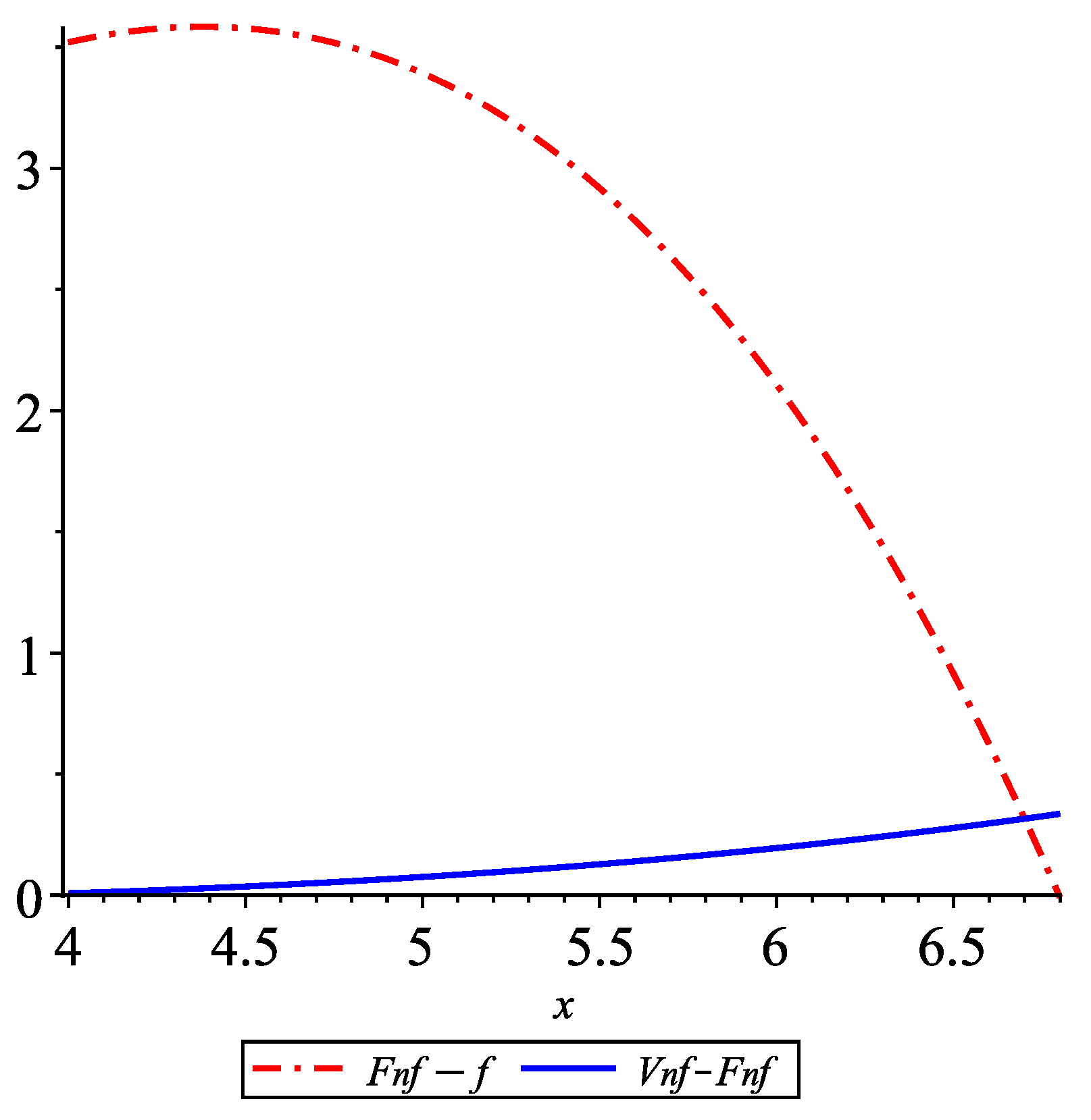
In what follows, we present numerical and graphical experiments comparatively illustrating the approximations furnished by the operators ${\mathcal{F}}_n$ and $V_n$. In our examples, ${\mathcal{F}}_n$ approximates better than $V_n$ on certain subintervals and for large values of n, but it is easy to construct similar examples in which $V_n$ provides a better approximation.

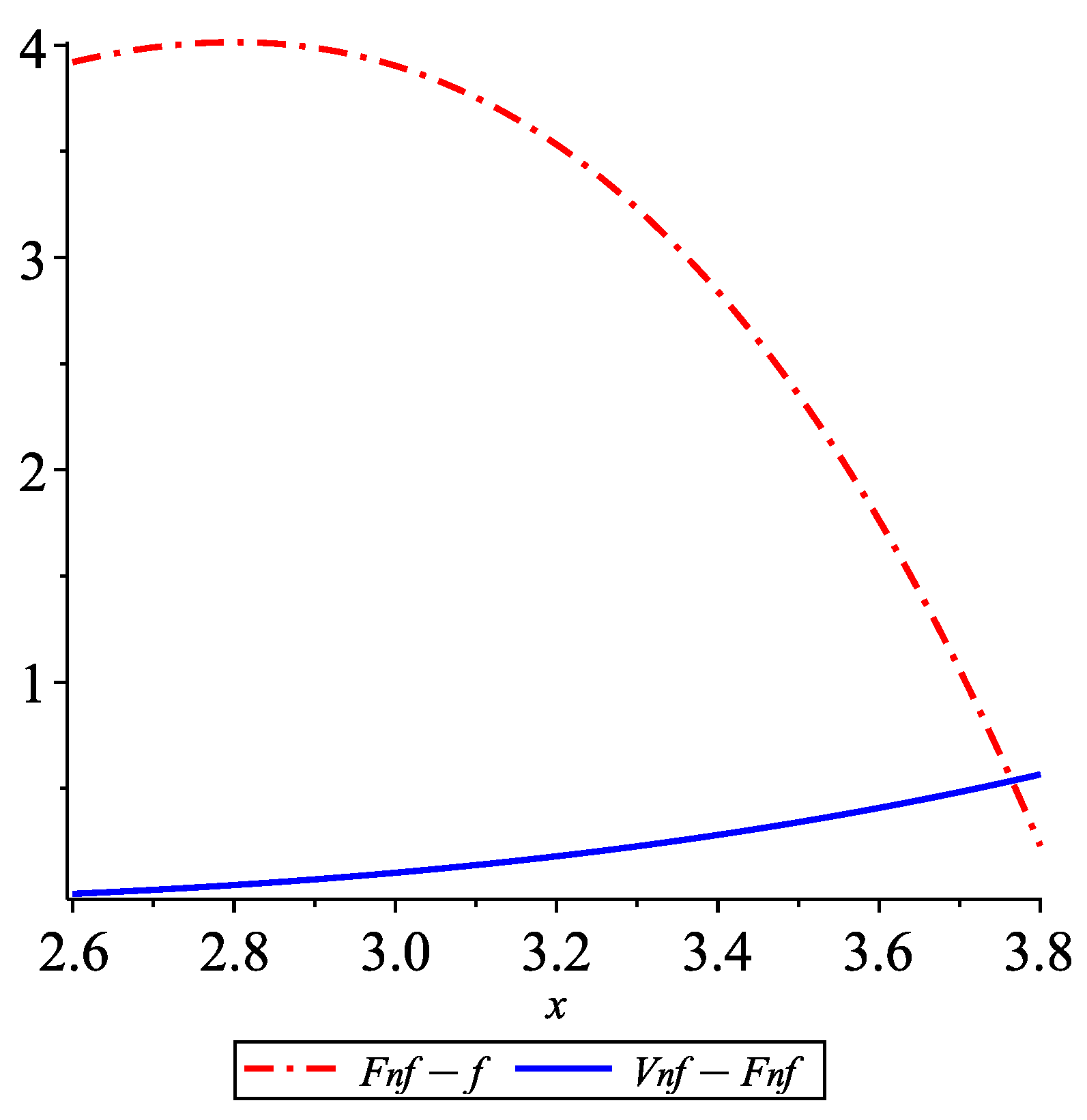
Example 1. 

Let $f\left(x\right)=21x^2-x^3$. Then, we have

$$\begin{array}{cc}\hfill {\mathcal{F}}_{n}f\left(x\right)& =-{\displaystyle \frac{x(nx+1)(nx-21n+44)}{(n-2)(n-1)}},\hfill \\ \hfill V_{n}f\left(x\right)& =-{\displaystyle \frac{x(n^2{x}^2-21n^{2}x+3n{x}^2-18nx+2x^2-21n+3x+1)}{n^2}}.\hfill \end{array}$$

Table 1. Error of approximation.

x	4	$4.1$	$4.2$	$4.3$	$4.4$	$4.5$
f	272	$284.089$	$296.352$	$308.783$	$321.376$	$334.125$
${\mathcal{F}}_{n}f$	$275.5204082$	$287.6380101$	$299.9214287$	$312.3642857$	$324.9602041$	$337.7028061$
$V_{n}f$	$275.5280000$	$287.6503912$	$299.9390016$	$312.3874664$	$324.9894208$	$337.7385000$
x	$4.6$	$4.7$	$4.8$	$4.9$	5	$5.1$
f	$347.024$	$360.067$	$373.248$	$386.561$	$400.000$	$413.559$
${\mathcal{F}}_{n}f$	$350.5857144$	$363.6025509$	$376.7469389$	$390.0125000$	$403.3928572$	$416.8816327$
$V_{n}f$	$350.6283392$	$363.6525736$	$376.8048384$	$390.0787688$	$403.4680000$	$416.9661672$
x	$5.2$	$5.3$	$5.4$	$5.5$	$5.6$	$5.7$
f	$427.232$	$441.013$	$454.896$	$468.875$	$482.944$	$497.097$
${\mathcal{F}}_{n}f$	$430.4724489$	$444.1589286$	$457.9346938$	$471.7933674$	$485.7285713$	$499.7339287$
$V_{n}f$	$430.5669056$	$444.2638504$	$458.0506368$	$471.9209000$	$485.8682752$	$499.8863976$
x	$5.8$	$5.9$	6	$6.1$	$6.2$	$6.3$
f	$511.328$	$525.631$	$540.000$	$554.429$	$568.912$	$583.443$
${\mathcal{F}}_{n}f$	$513.8030613$	$527.9295919$	$542.1071430$	$556.3293368$	$570.5897959$	$584.8821429$
$V_{n}f$	$513.9689024$	$528.1094248$	$542.3016000$	$556.5390632$	$570.8154496$	$585.1243944$

contains numerical values for $n=50$. We can remark that for this specific example the approximation provided by the operator ${\mathcal{F}}_n$ is better than that provided by $V_n$.

For $n=50$, Figure 1 illustrates the inequalities $f\le {\mathcal{F}}_{n}f\le V_{n}f$ on the subinterval [4,6.8].

Example 2. 

Let $f\left(x\right)=8x^3-x^4$. Then, we have

$$\begin{array}{cc}\hfill {\mathcal{F}}_{n}f\left(x\right)& =-{\displaystyle \frac{x(50x+1)(25x+1)(-373+50x)}{\mathrm{55,272}}},\hfill \\ \hfill V_{n}f\left(x\right)& =-{\displaystyle \frac{3x(\mathrm{46,852}{x}^3-\mathrm{348,296}{x}^2-\mathrm{20,281}x-133)}{\mathrm{125,000}}}.\hfill \end{array}$$

Table 2. Error of approximation.

x	$2.6$	$2.7$	$2.8$	$2.9$	3	$3.1$
f	$94.9104$	$104.3199$	$114.1504$	$124.3839$	$135.0000$	$145.9759$
${\mathcal{F}}_{n}f$	$98.83019976$	$108.3091186$	$118.1642857$	$128.3712766$	$138.9029526$	$149.7294616$
$V_{n}f$	$98.83372562$	$108.3314492$	$118.2091906$	$128.4428907$	$139.0057920$	$149.8684382$
x	$3.2$	$3.3$	$3.4$	$3.5$	$3.6$	$3.7$
f	$157.2864$	$168.9039$	$180.7984$	$192.9375$	$205.2864$	$217.8079$
${\mathcal{F}}_{n}f$	$160.8182371$	$172.1339992$	$183.6387538$	$195.2917934$	$207.0496961$	$218.8663265$
$V_{n}f$	$160.9986742$	$172.3616465$	$183.9198028$	$195.6328920$	$207.4579645$	$219.3493719$

contains numerical values for $n=50$. We can remark that for this specific example the approximation provided by the operator ${\mathcal{F}}_n$ is better than that provided by $V_n$.

For $n=50$, Figure 2 illustrates the inequalities $f\le {\mathcal{F}}_{n}f\le V_{n}f$ on the subinterval [2.6,3.8].

6. Conclusions and Further Work

Problems involving the composition and decomposition of positive linear operators are important in Approximation Theory. Information in this direction can be found, e.g., in the series of papers “Composition and decomposition of positive linear operators I–VII”. Our paper is the eighth in this series.

As explained in the introduction, the following types of problems were investigated in the literature concerning the composition and decomposition of positive linear operators: eigenstructures and the inverse of a composed operator, Voronovskaja-type formulas, the convergence of special modifications, and second-order central moments. We are concerned with some classical integral positive linear operators. For compositions of such operators, we investigate the problems mentioned above.

The new results are systematically presented in the sections of our paper. At the beginning of each section, our contribution is briefly described.

One can think to extend such results to more general families of operators and the more general context of weighted spaces presented in the papers [15,16]. A significant direction of research in the Approximation Theory by positive linear operators is concerned with the complete asymptotic expansion of such operators (see [17,18,19,20,21]). We intend to obtain such a complete asymptotic expansion for the composed operators investigated in this paper. Rates of convergence in approximation by positive linear operators were obtained for many sequences of operators (see, for example [22,23,24,25,26,27]). Quantitative results would also be interesting, of course, in the framework of the composed operators presented in this paper.