Impact of Goodwill on Consumer Buying through Advertising in a Segmented Market: An Optimal Control Theoretic Approach

Abstract

Market segmentation is one of the key marketing activities to target the potential market for a product, which allows the firm to have a better understanding of their customers. This paper considers an optimal control problem to determine the dynamic price and advertising policies of a new product introduction in a segment-specific market incorporating advertising-based goodwill. Under differentiated advertising and single-channel advertising, advertising efforts increase the stock of goodwill in each segment. Single-channel advertising starts in all segments with a fixed segment spectrum, while the differentiated advertising process deals with each segment independently. The explicit optimal dynamic advertising effort and price strategies are obtained by applying Pontryagin’s maximum principle, and local stability of equilibria have also been examined. The effectiveness of the proposed method is validated through numerical examples, and a local sensitivity analysis is performed to find the sensitive parameters that can affect the optimal values of price and advertising effort rates.

1. Introduction

The early stages of market penetration are important to a product’s future dissemination; therefore, introducing a new product into the market carries a significant degree of risk for the company. Many marketing efforts are focused on advertising methods that aid in the introduction of new products and have a positive effect on the diffusion curve. When launching a new product to the market, a company must identify the specific market segments that are more likely to acquire the product. They may differ in their needs, resources, locations, and buying attitudes. Customers in today’s international marketplaces are multicultural, with a wide range of tastes, needs, and desires. Despite the significant efforts put forth in creativity and advertising planning, meeting the demands of each client by treating them equally remains incredibly difficult and unpredictable. As a result, firms need to achieve this aim by dividing a particular market into distinct groups, and marketing strategies are designed accordingly. This necessitates the segmentation of markets into several market segments made up of clients with identical demand characteristics.

Market segmentation [1] is the process of partitioning the whole market into distinct consumer subgroups that behave in similar ways or have similar product needs. Market segmentation can be done in many ways using different segmentation variables to find the best way to view the market structure. The major variables—such as geographic (countries, nations, regions, cities, states, and neighborhoods), demographic (gender, age, income, education, family size, and occupation), psychographic (personality, social class, life style, and value), and behavioral (user states, usage rate, purchase occasion, and attitude towards product)—are some useful segmentation characteristics or attributes. If each consumer segment is fairly homogenous in its unique requirement, it is likely to respond similarly to a given marketing strategy and assist firms in better understanding and satisfying their customers. After market segmentation, firms identify various segments and develop a marketing mix strategy for each segment. Simultaneously, business establishments follow mass market advertising strategies that reach diverse segments with a fixed spectrum, as well as segment-specific advertising strategies.

It is a well-known fact that market segmentation is an integral part of marketing theory and practice, as well as a vital aspect of a company’s success in the current era. It has a huge impact on customer demand and reminds us of the importance of using a variety of advertising media channels to target consumers with varying media preferences [2]. Even though many researchers [1,2,3,4,5,6] have emphasized the need of market segmentation in marketing literature, only a few mathematical models in advertising-based goodwill deal with market segmentation [7,8,9,10,11]. Little and Lodish [7] investigated the stochastic model in a segmented market that included the concept of multiple media selection in a discrete time horizon. Seidmann et al. [8] addressed interfaces between sales and advertising dynamics in a distributed sales-advertising model, where the system constitutes population distribution over a parameter space. With Nerlove and Arrow’s [12] linear goodwill dynamics, Buratto et al. [9,11] incorporate some market segmentation ideas into advertising models when addressing the introduction of a new product and an advertising channel selection problem in a segmented market.

Jha et al. [13] explored the optimal advertising effectiveness rate in a segmented market by incorporating market segmentation into a diffusion model that considered advertising for a product. Favaretto and Viscolani [10] explored an optimal control model relying on advertising and production for a seasonal product using Nerlove–Arrow’s linear goodwill dynamics in a segmented market. Mehta et al. [14] used an innovation diffusion model to determine the optimal promotion efforts to make when a new product is launched in a segmented market with changing market size. The authors assumed that the market size was dynamic, as well as that the market was segmented. Ma and Jiang [15] proposed an advertising model in which they have investigated a single-parameter sales promotion strategy, and they analyzed the stability of their proposed model. Chaudhary et al. [16] have addressed the optimal control problem to determine the optimal promotional policies of a diffusion model in a segmented market and to analyze the stability of their model under the assumption that the new product’s additional demand improves the brand image of the firm in the form of goodwill.

In the marketing literature dealing with goodwill formulation, models based on the Nerlove–Arrow model’s dynamics are extremely common. In line with the researchers [9,10,11,12,17] in marketing literature involving advertising goodwill accumulation in a segmented environment, our advertising-based goodwill model also relies on the framework of Nerlove–Arrow’s model. Firms advertise their products in both national and local regional languages in order to reach a vast customer base, especially in culturally diverse countries, where each region is influenced by a defined spectrum of national language. We widen the scope of goodwill formulation in this work by considering a differentiated and a single-channel advertising strategy simultaneously in a segmented market, with the objective of maximizing its profit. Price and advertising-based goodwill are expected to drive the sales rate function. We investigate a linear sales rate function that drops in price, while increasing in goodwill stock. We have assumed that the firm/company has defined its target market as a segmented market and has decided to create distinct and single-channel advertising campaigns for each segment at the same time in order to maximize profits. The optimal dynamic price and advertising policies are developed using an optimal control theory technique. Vast literature [18,19,20,21,22,23,24] exists in marketing on dynamic advertising and pricing policies for sales and advertising models using an optimal control theoretic approach.

The aim of this study is to examine the impact of advertising-based goodwill on the sales of a new product and fill the gap by determining the differentiated and single-channel advertising strategies in a segmented market. This paper provides an optimal advertising policy, which advocates for firms to begin with a heavy advertising effort in order to give momentum to the goodwill evolution process. The differentiated and single-channel advertising efforts are gradually diminished, and perhaps no advertising efforts should be utilized at a terminal interval of time. This outcome is caused by word-of-mouth impact; advertising efforts are used to build an initial stock of goodwill for the product, but as the word-of-mouth increases, advertising efforts decrease.

The rest of the paper is structured as follows. In Section 2, a mathematical optimal control model is developed for the evolution of advertising-based goodwill and formulated as an optimum control problem under the premise that differentiated and single-channel advertising processes occur simultaneously. Applying Pontryagin’s maximum principle in Section 3 yields the dynamic advertising and pricing plan for each segment. Section 4 contains numerical examples and a local sensitivity analysis. The paper concludes in Section 5.

2. Model Formulation

We consider a monopolist firm that needs to define its targeted and defined market in a segmented population of consumers and plan the differentiated and single-channel advertising strategies simultaneously, with the objective to maximize its total profit. We assume that advertising begins simultaneously, and there are enough products to meet the demand in each segment. The differentiated advertising process can reach each segment selectively, and the single-channel advertising process has an effectiveness segment spectrum that is distributed over the set of segments (that reaches with a fixed spectrum in each segment). Here, we assume that the whole market is divided into $N$ market segments, $N$ is a discrete variable, and each segment is specified by the geographic segmentation attributes (countries, nations, regions, cities, states, etc.) as discussed by Kotler [1]. Let $\left[0,T\right]$ be the planning period of the differentiated and single-channel advertising efforts for the new product introduction. Let $y_i\left(t\right)$ be the stock of the product’s goodwill level at time $t\in \left[0,T\right]$ for the $i^{th}$ segment, and $w_i\left(t\right)$ and $w\left(t\right)$ are the differentiated and single-channel advertising effectiveness effort rates at time $t$ that influence the goodwill of the product. We use Nerlove and Arrow’s [11] definition of “goodwill” to describe a variable that sums the effects of current and previous advertising or promotions on sales and, as a result, its current and future net revenues. While goodwill deteriorates naturally, it can be increased through advertising efforts. Under the combined effects of differentiated and single-channel advertising, the evolution of goodwill can be expressed as:

$$\frac{d{y}_i\left(t\right)}{dt}=\left(w_i\left(t\right)+{\alpha }_{i}w\left(t\right)\right)-{\delta }_i y_i\left(t\right), y_i\left(0\right)=y_{i0} i=1,2,\dots ,N$$

(1)

Single-channel advertising’s segment-effectiveness varies depending on the market segment, and different market segments require different levels of advertising effort rate. Here ${\alpha }_i>0; {{\displaystyle \sum }}_i{\alpha }_i=1, \forall i=1\dots N,$ is the single channel’s spectrum; ${\delta }_i>0$ represents the rate of goodwill depreciation for the $i^{th}$ segment; the left-hand side of Equation (1) shows the change in goodwill. The first term describes the level of goodwill increase due to joint advertising efforts using differentiated and single-channel advertising, while the second term shows that it depreciates over time at rate ${\delta }_i$ due to consumers drifting away to other brands, new brands, etc.

To formulate an optimal control model for a monopolistic firm, suppose that the sales rate depends on the price $p_i\left(t\right)$ and the stock of goodwill $y_i\left(t\right),$ so that the sales rate function for the $i^{th}$ segment presented in Pan and Li [25] is adopted as:

$$\frac{d{s}_i}{dt}=a_i-a_{1i}{p}_i\left(t\right)+a_{2i}{y}_i\left(t\right)$$

(2)

where $a_i>0$ represents the initial market size (market potential), and $a_{1i}>0$ and $a_{2i}>0$ represent the customer pricing and goodwill sensitivity for the $i^{th}$ segment, respectively. Equation (2) states that the sales rate will be positive for given values of $a_i, a_{1i},$ and $a_{2i}$ if the combined impact of the market potential and goodwill, $a_i+a_{2i}{y}_i\left(t\right)$, is greater than the impact of the price, $a_{1i}{p}_i\left(t\right)$. The sales rates decrease with the price but increase with the goodwill of the product. Let $c_i\left(t\right)$ be the per unit sales production cost, and for simplicity, $c_i\left(t\right)=c_i$ is a constant for each segment. The amount of money spent on differentiated and single-channel advertising determines how well the company meets its sales or profit goals. As a result, we can express the optimal control policy of identifying the optimal differentiated and single-channel advertising effort rates ($w_i\left(t\right), w\left(t\right)$) for the new product as follows:

$$Max J={{\displaystyle \int }}_0^T{e}^{-rt}\left({{\displaystyle \sum }}_{i=1}^N \left[\left(p_i\left(t\right)-c_i\right){\dot{s}}_i\left(t\right)-{\varphi }_i\left(w_i\left(t\right)\right)\right]-\phi \left(w\left(t\right)\right)\right)dt$$

(3)

subjected to state Equation (1), where ${\varphi }_i(w_i\left(t\right)$) denotes the cost of differentiated advertising, $\phi \left(w\left(t\right)\right)$ the cost of single-channel advertising, and $r$ the rate of profit discounting.

The differentiated and single-channel advertising efforts are expensive, and we assume that both advertising effort cost functions are quadratic, ${\varphi }_i\left(w_i\right)=\frac{k_i}{2}{w}_i^2\left(t\right)$ and $\phi \left(w\left(t\right)\right)=\frac{k}{2}{w}^2\left(t\right)$, where ${\kappa }_i>0$ and $\kappa >0$ are constants and denote the magnitude of the advertising effort rates per unit of time towards the $i^{th}$ segment and single-channel advertising, respectively. This is a very common assumption in the literature, as discussed in Teng and Thompson [20], Ouardighi and Pasin [26], and Chaudhary et al. [16], where the advertising cost is quadratic. Combining the objective function Equation (3), state Equation (1), and sales rate function (2), the optimization problem can be defined as an optimal control problem:

$$\left.\begin{array}{c}Max J={{\displaystyle \int }}_0^T{e}^{-rt}\left({{\displaystyle \sum }}_{i=1}^N\left[ \left(p_i\left(t\right)-c_i\right) \dot{s_i}\left(t\right)-\frac{k_i}{2}{w}_i^2\left(t\right)\right]-\frac{k}{2}{w}^2\left(t\right)\right) dt\\ \frac{d{y}_i\left(t\right)}{dt}=\left(w_i\left(t\right)+{\alpha }_{i}w\left(t\right)\right)-{\delta }_i{y}_i\left(t\right), y_i\left(0\right)=y_{i0} i=1,2,\dots ,N\end{array}\right\}$$

(4)

In the model described by expression (4), the control variables are advertising effort rates $w_i\left(t\right)$, $w\left(t\right),$ and price $p_i\left(t\right)$, and stock of goodwill for each segment $y_i\left(t\right)$ are state variables.

3. Optimal Policy and Local Stability Analysis

First, we use the maximum principle in its current value formulation to determine the optimal policies for pricing and advertising. Then, we derive the local stability analysis of the state–costate phase plane.

3.1. Optimal Dynamic Strategy for Finite Time Horizon

To obtain the dynamic advertising and pricing strategy, we solve Equation (4), which is the optimal control problem, using Pontryagin’s maximum principle as stated in Sethi and Thompson [19]. The Hamiltonian function is defined as:

$$H\left(y_i,w_i,w,p_i,{\lambda }_i\right)={{\displaystyle \sum }}_{i=1}^N\left[ \left(p_i-c_i\right) \left(a_i-a_{1i}{p}_i+a_{2i}{y}_i\right)-\frac{k_i}{2}{w}_i^2\right]-\frac{k}{2}{w}^2+{{\displaystyle \sum }}_{i=1}^N{\lambda }_i\left(w_i+{\alpha }_{i}w-{\delta }_i{y}_i\right)$$

(5)

where ${\lambda }_i$ represent the adjoint variables. The instantaneous profit rate is represented by the Hamiltonian function in Equation (5), that is the sum of two parts. First part, ${{\displaystyle \sum }}_{i=1}^N\left[ \left(p_i-c_i\right) \left(a_i-a_{1i}{p}_i+a_{2i}{y}_i\right)-\frac{k_i}{2}{w}_i^2\right],$ represents current profit and second part, ${{\displaystyle \sum }}_{i=1}^N{\lambda }_i\left(w_i+{\alpha }_{i}w-{\delta }_i{y}_i\right),$ which consists of adjoint variables, represents future profit. We are primarily interested in the shape of optimal solutions in the interior of control. If $w_i^{*}\left(t\right)>0$, $w^{*}\left(t\right)>0$ and $p_i^{*}\left(t\right)$ exist and are optimal solutions to Equation (4), the Maximum Principle defined by Sethi and Thompson [19] and Seierstad and Sydsaeter [27] provides the required optimality conditions. For $w_i^{*}\left(t\right), w^{*}\left(t\right), p_i^{*}\left(t\right)$ with the corresponding optimal state trajectory $y_i^{*}\left(t\right)$, there exist continuous and piecewise continuously differentiable functions ${\lambda }_i\left(t\right)$ for all $tϵ\left[0,T\right],$ such that:

$$\frac{\partial H}{\partial w_i^{*}}=0 \forall i ϵ N, \frac{\partial H}{\partial w^{*}}=0, \frac{\partial H}{\partial p_i^{*}}=0 \forall i ϵ N$$

(6)

The terminal conditions of the state variables $y_i\left(T\right)$ are not restricted. The adjoint variables ${\lambda }_i$ satisfy the following differential equation:

$$\frac{d}{dt}{\lambda }_i=r{\lambda }_i-\frac{\partial H}{\partial y_i}, \forall i ϵ N$$

(7)

with the transversality conditions ${\lambda }_i\left(T\right)=0$.

Since $k_i, k,$ and $a_{1i}$ are parameters, and all are positive constant, for the optimal control problem (4), the following sufficient conditions hold:

$$\frac{{\partial }^{2}H}{\partial w_i^2}=-k_i<0, \frac{{\partial }^{2}H}{\partial w^2}=-k<0, \frac{{\partial }^{2}H}{\partial p_i^2}=-2a_{1i}<0$$

(8)

$$\frac{{\partial }^{2}H}{\partial w_i^2}\frac{{\partial }^{2}H}{\partial w^2}-{\left(\frac{{\partial }^{2}H}{\partial w{w}_i}\right)}^2>0$$

(9)

$$\frac{{\partial }^{2}H}{\partial w_i^2}\frac{{\partial }^{2}H}{\partial p_i^2}-{\left(\frac{{\partial }^{2}H}{\partial w_i{p}_i}\right)}^2>0$$

(10)

$$\frac{{\partial }^{2}H}{\partial p_i^2}\frac{{\partial }^{2}H}{\partial w^2}-{\left(\frac{{\partial }^{2}H}{\partial w{p}_i}\right)}^2>0$$

(11)

Hence, the Hamiltonian is a concave function in $w_i, p_i,$ and $w$ for each of the segments, and the maximization yield is a unique control variable.

Solving differential Equation (7) for the adjoint variable, we have (See Appendix A):

$${\lambda }_i\left(t\right)=\frac{a_{2i}{c}_i}{ \left({\eta }_i-1\right) \left(r+{\delta }_i\right)}\left(1-e^{-\left(r+{\delta }_i\right)\left(T-t\right)}\right)$$

(12)

The adjoint variables ${\lambda }_i\left(t\right)$ represent the marginal value (shadow price) of the goodwill level $y_i\left(t\right)$ and determine the shadow price of an additional unit of the goodwill along the optimal trajectory. According to the optimality conditions in (6), as discussed in Seierstad and Sydsaeter [27], one can obtain the optimal advertising efforts rate $w_i^{*}\left(t\right), w\left(t\right),$ and price strategy $p_i^{*}\left(t\right)$ as (See Appendix A):

$$w_i^{*}=\frac{a_{2i} c_i}{k_i ({\eta }_i-1) \left(r+{\delta }_i\right)}\left(1-e^{-\left(r+{\delta }_i\right)\left(T-t\right)}\right)$$

(13)

$$w^{*}\left(t\right)=\frac{1}{k}\left({\displaystyle \sum }_{i=1}^N\left[ \frac{ {\alpha }_i a_{2i} c_i}{ \left({\eta }_i-1\right) \left(r+{\delta }_i\right)}\left(1-e^{-\left(r+{\delta }_i\right)\left(T-t\right)}\right)\right]\right)$$

(14)

$$p_i^{*}=\frac{ c_i {\eta }_i}{\left({\eta }_i-1\right)}$$

(15)

where ${\eta }_i=-\frac{\frac{\partial \dot{s_i}}{\partial p_i}}{\frac{\dot{s_i}}{p_i}}$ is the demand elasticity with respect to price. The results of Equation (15) are generalisations of the myopically optimal price rule for a monopolist, as used in the price literature [28]; ${\eta }_i>1$. The optimal pricing policy $p_i^{*}$ is the usual price formula for the monopolist. From the above expressions (13) and (14), we see that the optimal value of advertising efforts decreases over time interval $\left[0,T\right]$. We perceive that the advertising effort for all the segments decreases as time passes by. Moreover, near the end of the planning period, it is optimal to advertise at low levels. This result is due to the goodwill effect of the product; advertising efforts are used to enhance and generate the goodwill, but as the goodwill of the product gains impulsion, the advertising need is less near the end of the planning period, $T$.

For the optimal control policy, the optimal goodwill trajectory using optimal values of the differentiated advertising effort rates $w_i^{*}\left(t\right)$ and the single-channel advertising effort $w_i^{*}\left(t\right)$ rate from Equations (13) and (14) for each segment are given by:

$$y_i^{*}\left(t\right)=y_{i0} e^{-{\delta }_{i}t}+{{\displaystyle \int }}_0^t\left(w_i^{*}\left(t\right)+{\alpha }_i w^{*}\left(t\right)\right)e^{-{\delta }_i\left(t-\tau \right)}d\tau \forall i$$

(16)

If $y_i\left(0\right)=0$, then the following result is obtained:

$$y_i{}^{*}\left(t\right)={{\displaystyle \int }}_0^t\left(w_i^{*}\left(t\right)+{\alpha }_i w^{*}\left(t\right)\right)e^{-{\delta }_i\left(t-\tau \right)}d\tau \forall i$$

(17)

3.2. Optimal Dynamic Strategy for Infinite Time Horizon

For infinite horizon problems, the objective functional is given by

$$Max J={{\displaystyle \int }}_0^{\infty }{e}^{-rt}\left({{\displaystyle \sum }}_{i=1}^N\left[ \left(p_i\left(t\right)-c_i\right) \dot{s_i}\left(t\right)-\frac{k_i}{2}{w}_i^2\left(t\right)\right]-\frac{k}{2}{w}^2\left(t\right)\right) dt$$

(18)

The function $f\left(w_i.w, p_i,y_i\right)=\left({{\displaystyle \sum }}_{i=1}^N\left[ \left(p_i\left(t\right)-c_i\right) \left(a_i-a_{1i}{p}_i\left(t\right)+a_{2i}{y}_i\left(t\right)\right)-\frac{k_i}{2}{w}_i^2\left(t\right)\right]-\frac{k}{2}{w}^2\left(t\right)\right)$ is regarded as being bounded for any solution to Equation (1). Then, the integral in Equation (18) converges for all admissible pairs. The infinite horizon problem discussed in Equations (1) and (2), along with objective function, which is defined by Equation (18), provide the optimal solution of the given system. The Pontryagin Maximum Principle’s optimality conditions for finite-horizon, apart from the transversality condition, carry over to the infinite-horizon problem by taking the limit for $T\to \infty$ [27]. With the current-value adjoint variable, the Hamiltonian function given in Equation (5) satisfies the first order differential equation for each segment:

$$\frac{d}{dt}{\lambda }_i=r{\lambda }_i-\frac{\partial H}{\partial y_i}, \forall i ϵ N$$

(19)

and the condition of transversality:

$$\underset{T\to \infty }{\mathit{lim}}{e}^{-rT}{\lambda }_i\left(T\right)=0$$

(20)

Equation (19) represents the equilibrium relation for goodwill investment. It states that the marginal opportunity cost ${\lambda }_i\left({\rho }_i+{\delta }_i\right)dt$ of investment in goodwill should be equal to the marginal profit $\left(p_i-c_i\right)a_{2i}$ from the increased goodwill and the capital gain $\dot{{\lambda }_i}$ [11]. We use $\dot{y_i}=0, \dot{{\lambda }_i}=0, H_{w_i}=0, and H_w=0$ to obtain the optimal long-run equilibrium [19] or turnpike $\left(\overline{y_i}, \overline{w_i}, \overline{w},\overline{{\lambda }_i}\right)$ of the Hamiltonian system and equilibrium control. We have:

$$\overline{{\lambda }_i}=\frac{c_i{a}_{2i}}{\left({\eta }_i-1\right)\left(r+\delta \_\right)}$$

(21)

$$\overline{w_i}=\frac{1}{k_i}\frac{c_i{a}_{2i}}{\left({\eta }_i-1\right)\left(r+\delta \right)}$$

(22)

$$\overline{w}=\frac{1}{k}{\displaystyle \sum }_{i=1}^N\frac{{\alpha }_i c_i{a}_{2i}}{\left({\eta }_i-1\right)\left(r+\delta \right)}$$

(23)

$$\overline{y_i}=\frac{1}{{\delta }_i}\left(\frac{1}{k_i}\frac{c_i{a}_{2i}}{\left({\eta }_i-1\right)\left(r+\delta \right)}+\frac{{\alpha }_i}{k}{\displaystyle \sum }_{i=1}^N\frac{{\alpha }_i c_i{a}_{2i}}{\left({\eta }_i-1\right)\left(r+\delta \right)} \right)$$

(24)

The property of $\overline{y_i}$ indicates that the optimal policy is to go to $\overline{y_i}$ as quickly as possible. For $y_i\left(0\right)>\overline{y_i}$, the optimal control is $w_i^{*}\left(t\right)=0, w^{*}\left(t\right)=0$, untill the stock of goodwill has depreciated to $\overline{y_i}$, at which time the control switches to $\overline{w_i}=\frac{1}{k_i}\frac{c_i{a}_{2i}}{\left({\eta }_i-1\right)\left(r+\delta \right)}, \overline{w}=\frac{1}{k}{\displaystyle \sum }_{i=1}^N\frac{{\alpha }_i c_i{a}_{2i}}{\left({\eta }_i-1\right)\left(r+\delta \right)}$ and remains at this level to maintain the level of goodwill $\overline{y_i},$ i.e., the optimal policy is to be advertised at a low rate initially and gradually increase advertising to the turnpike level $\overline{w_i}, \overline{w}$. For $y_i\left(0\right)<\overline{y_i}$, it is optimal to jump to $\overline{y_i}$ immediately by using the appropriate impluse at time $t=0$ and then set $\overline{w_i}=\frac{1}{k_i}\frac{c_i{a}_{2i}}{\left({\eta }_i-1\right)\left(r+\delta \right)}, \overline{w}=\frac{1}{k}{\displaystyle \sum }_{i=1}^N\frac{{\alpha }_i c_i{a}_{2i}}{\left({\eta }_i-1\right)\left(r+\delta \right)}$ for $t>0,$ i.e., the optimal policy is to advertise most heavily initially and gradually decease advertising to the turnpike level $\overline{w_i}, \overline{w}$ as $y_i$ approaches $\overline{y_i}$. Figure 1 depicts the graph of the optimal policy for two initial conditions.

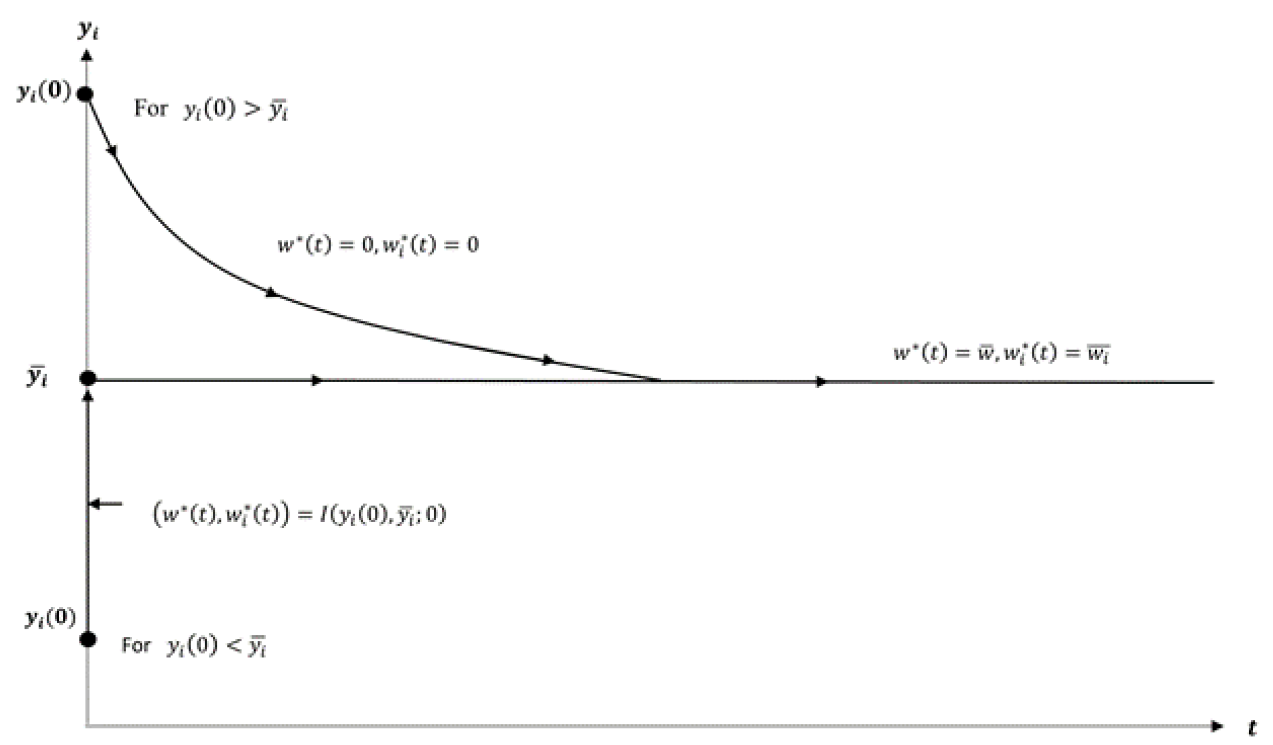
3.3. Local Stability Analysis in the State–Costate-Phase Plane

An equilibrium for a state–costate system defined by $\dot{y}\left(t\right)=\dot{{\lambda }_i}\left(t\right)=0$ plays an important role in the determination of the optimal policy. In this section, we discuss the local stability analysis of the nontrivial equilibrium point $E^{*}\left(y_i^{*},{\lambda }_i^{*}\right)$ to show how small changes in sales and goodwill values affect the local profit and stabilization. Now, we turn to determining the optimal trajectories in the $\left(y_i,{\lambda }_i\right)$-phase diagram. By using condition (6), we obtain the following system of differential equations:

$$\frac{d{y}_i}{dt}=\left(\frac{1}{k_i}{\lambda }_i\left(t\right)+\frac{{\alpha }_i}{k}{\displaystyle \sum }_{i=1}^N{\alpha }_i{\lambda }_i\left(t\right)\right)-{\delta }_i{y}_i\left(t\right)$$

(25)

$$\frac{d{\lambda }_i}{dt}=\left(r+{\delta }_i\right){\lambda }_i-\frac{C_i{a}_{2i}}{{\eta }_i-1}$$

(26)

The Jacobian matrix of system Equations (25) and (26) can be determined as:

$$\frac{\partial \dot{y_i}}{\partial y_i}=-{\delta }_i<0, \frac{\partial \dot{y_i}}{\partial {\lambda }_i}=\left(\frac{1}{k_i}+\frac{{\alpha }_i^2}{k}\right)>0, \frac{\partial \dot{{\lambda }_i}}{\partial y_i}=0, \frac{\partial \dot{{\lambda }_i}}{\partial {\lambda }_i}=\left(r+{\delta }_i\right)>0$$

(27)

Hence, the determinant of the Jacobian $\frac{\partial \dot{y_i}}{\partial y_i}\frac{\partial \dot{{\lambda }_i}}{\partial {\lambda }_i}-\frac{\partial \dot{y_i}}{\partial {\lambda }_i}\frac{\partial \dot{{\lambda }_i}}{\partial y_i}<0,$ therefore, the equilibrium point $\left(y_i^{\infty },{\lambda }_i^{\infty }\right)$ is a saddle point, where ${\lambda }_i^{\infty }=\frac{c_i{a}_{2i}}{\left({\eta }_i-1\right)\left(r+\delta \_\right)}$ and

$$y_i^{\infty }=\frac{1}{{\delta }_i}\left(\frac{1}{k_i}\frac{c_i{a}_{2i}}{\left({\eta }_i-1\right)\left(r+\delta \right)}+\frac{{\alpha }_i}{k}{\displaystyle \sum }_{i=1}^N\frac{{\alpha }_i c_i{a}_{2i}}{\left({\eta }_i-1\right)\left(r+\delta \right)} \right)$$

Since no diagonal entries change signs in the Jacobian matrix, and the Jacobian does not vanish, according to Gale and Nikaido [29], the equilibrium point is unique. If the goodwill of the product $y_i$ is already high, then the shadow price ${\lambda }_i$ is comparatively low, whereas in the case of a low level of goodwill, an additional unit of goodwill is worth much more. As time tends to infinity, both the goodwill $y_i$ and the shadow price ${\lambda }_i$ approach their equilibrium values. The shadow price is a monotonically decreasing function over the finite planning period and does not depend on the stock of product goodwill (Huang et al. [23]).

The model is solved numerically in the next section with the help of an example, and a local sensitivity analysis is performed to see how the parameters and coefficient affect the optimal pricing and advertising effort values.

4. Numerical Illustration and Sensitivity Analysis

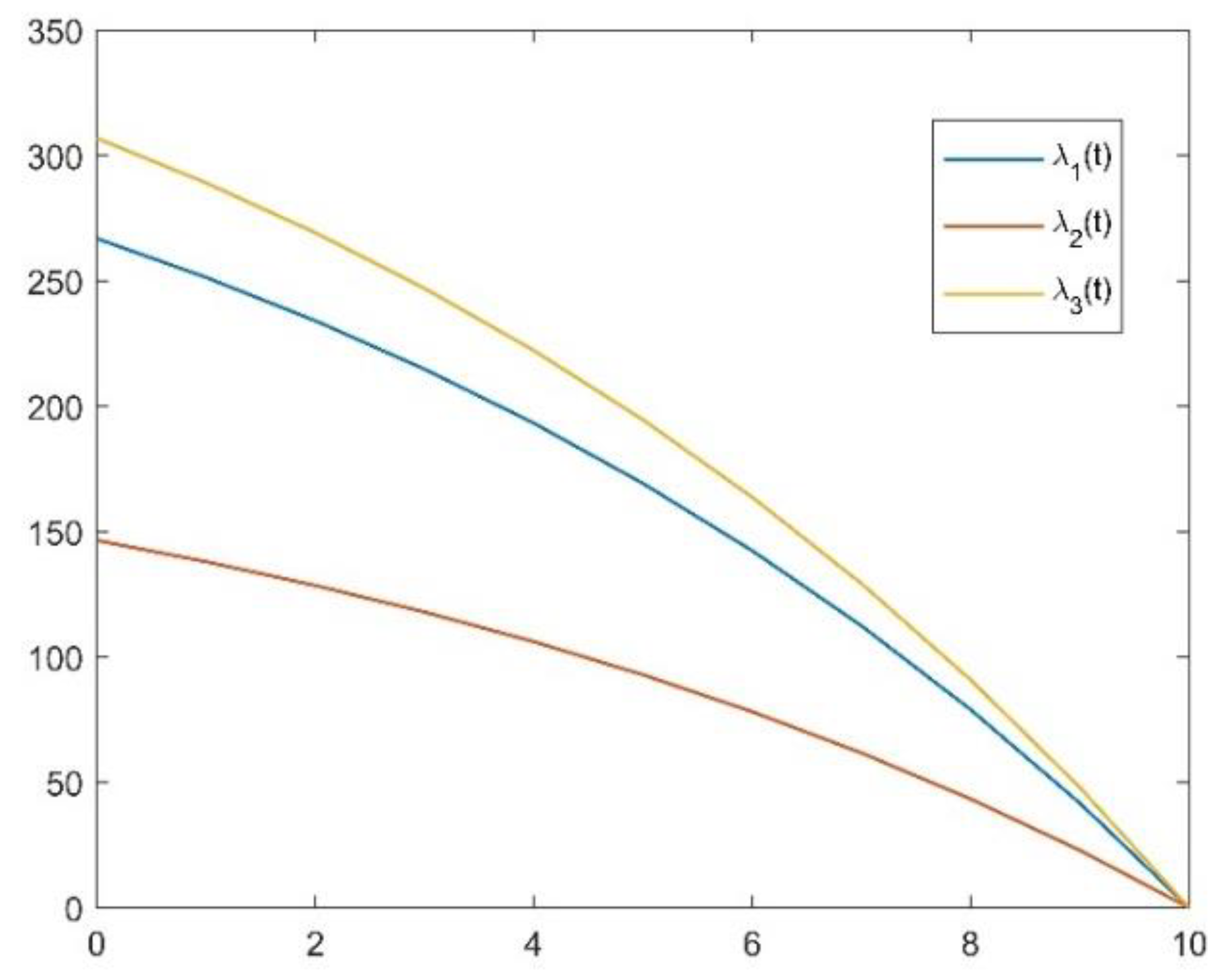
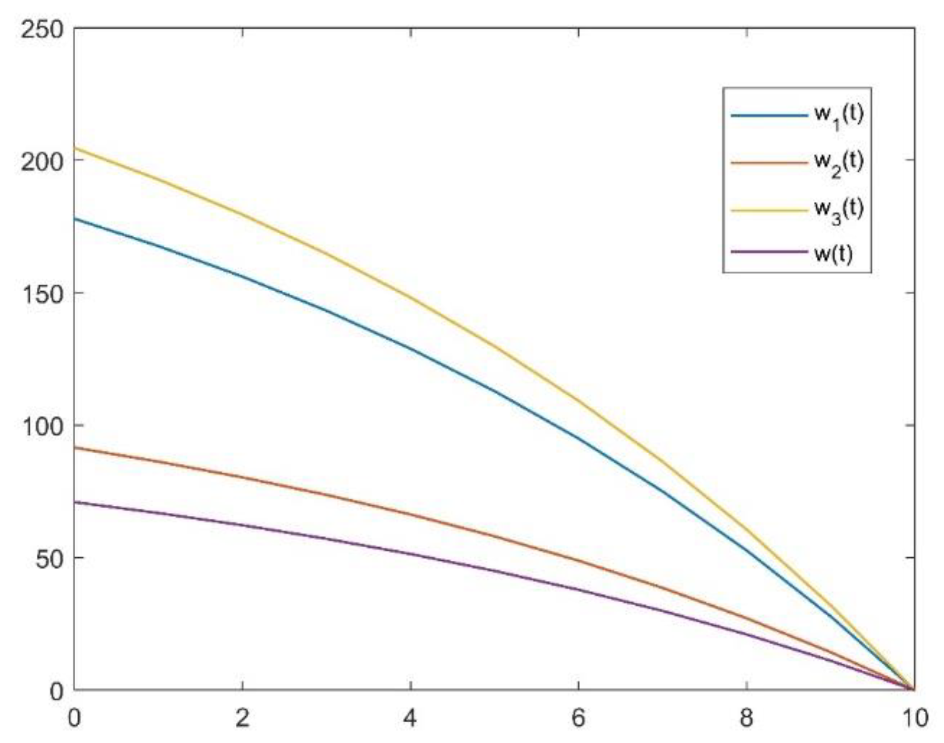
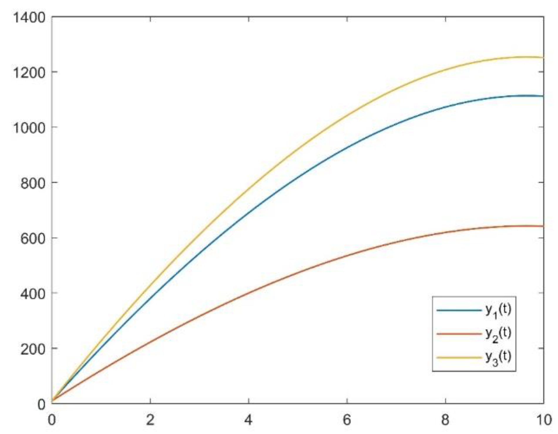
4.1. Numerical Illustrations

To illustrate the solution procedure and theoretical results, numerical examples and a sensitivity analysis are presented. Furthermore, key parameters’ sensitivity is analyzed. Firms advertised their products or services in national, as well as regional, languages to make people aware and influence maximum customers in multicultural and diverse countries, where the national language influences all regions within a fixed spectrum. We suppose that the time horizon is divided into 10 equal time periods. We have assumed the number of market segments are 3 (i.e., $N=3$), the discount rate $r=0.1,$ and $k=3$. The rest of the parameters used throughout the solution of the numerical examples are presented in

Table 1. Parameters used in numerical examples.

Segment	${\mathit{a}}_{\mathit{i}}$	${\mathit{a}}_{\mathit{i}}$	${\mathit{a}}_{1\mathit{i}}$	${\mathit{a}}_{2\mathit{i}}$	${\mathit{c}}_{\mathit{i}}$	${\mathit{\delta }}_{\mathit{i}}$	${\mathit{\eta }}_{\mathit{i}}$	${\mathit{k}}_{\mathit{i}}$
S1	1660	0.30	2.5	2.2	20	0.01	2	1.5
S2	1670	0.32	2.3	2.3	21	0.01	3	1.6
S3	1670	0.28	2.4	2.2	23	0.01	2	1.5

.

By using the expressions (13), (14) for $w_i^{*}\left(t\right), w^{*}\left(t\right),$ expression (15) for $p_i^{*},$ expression (17) for $y_i^{*}\left(t\right),$ and values of the parameters given in Table 1, the optimal value of the objective function is 494,740 units. The graphs of the adjoint variables, optimal advertising efforts rates, goodwill evolution, and profit function over time are shown in Figure 2, Figure 3, Figure 4 and Figure 5.

The above Figure 2 depicts that the graph of the adjoint decreasing functions ${\lambda }_i\left(t\right)$ for each segment is positive, but the decreasing function that demonstrates the future benefit of having one more unit of goodwill is always positive. Figure 3 demonstrates the graph of the optimal differentiated $w_i^{*}\left(t\right)$ and mass promotion effort rates $w^{*}\left(t\right)$ in each segment. Initially, the promotional effort rates displayed in Figure 3 are at a maximum level and decrease over time for all segments. As the goodwill level of the product gains momentum and approaches the end of planning period, then the decision maker should reduce the promotional effort level. Figure 4 shows the stock of goodwill of the product $y_i^{*}\left(t\right)$ for each segment. As shown in Figure 4, it is observed that the level of goodwill starts from the initial value and then increases in a concave curve pattern as time increases. The reason for this concave pattern is that growth rate of the goodwill of the product is proportional to the promotional effort rates. As the optimal promotional effort policy shows, initially we use the maximum promotional effort rates to stimulate the stock of goodwill. Figure 5 shows the $\left(y_1,y_2,y_3\right)$-phase diagram.

The local stability analysis for the system is obtained for the numerical values mentioned in Table 1. The equilibrium point obtained is $E^{*}\left(\text{29,857.21}, \text{17,124.84}, \text{33,644.51}\right),$ which is locally unstable, as the eigenvalues are ${\lambda }_1=-{\delta }_{i }, {\lambda }_2=r+{\delta }_{i,}$ which shows that the trajectories are attracting corresponding to the negative eigenvalue, but repulsive corresponding to the positive eigenvalue.

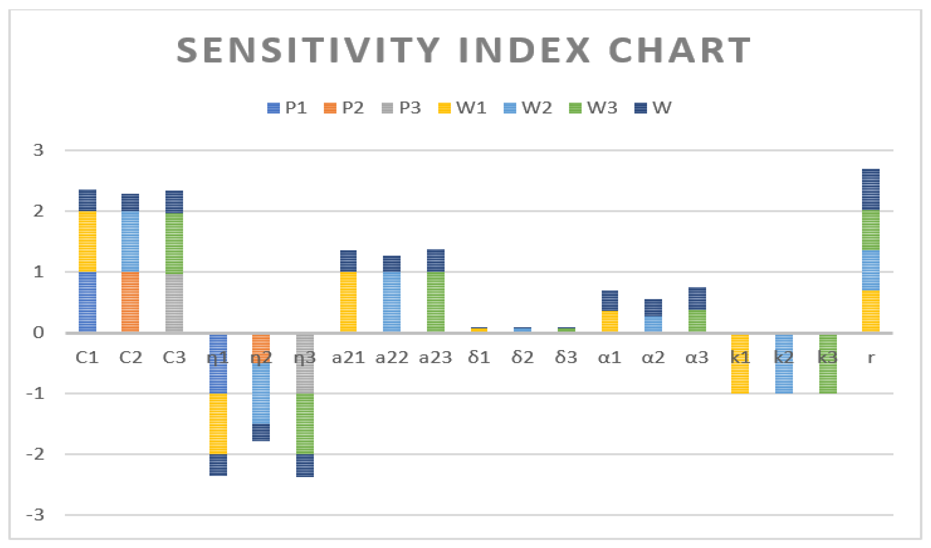
4.2. Local Sensitivity Analysis

In this sub-section, we have discussed the local sensitivity analysis for the proposed model to evaluate the important parameters whose variation can change the dynamics of the advertising and pricing of the system.

Table 2. Sensitivity Index.

Parameters	${\mathit{p}}_1$	${\mathit{p}}_2$	${\mathit{p}}_3$	${\mathit{w}}_1$	${\mathit{w}}_2$	${\mathit{w}}_3$	w
$c_1$	1	0	0	1	0	0	0.3504
$c_2$	0	1	0	0	1	0	0.2735
$c_3$	0	0	0.9565	0	0	1	0.3761
${\eta }_1$	−1	0	0	−1	0	0	−0.3504
${\eta }_2$	0	−0.5	0	0	−1	0	−0.2735
${\eta }_3$	0	0	−1	0	0	−1	−0.3761
$a_{21}$	0	0	0	1	0	0	0.3504
$a_{22}$	0	0	0	0	1	0	0.2735
$a_{23}$	0	0	0	0	0	1	0.3761
${\delta }_1$	0	0	0	0.0645	0	0	0.0236
${\delta }_2$	0	0	0	0	0.0673	0	0.0184
${\delta }_3$	0	0	0	0	0	0.0655	0.0253
${\alpha }_1$	0	0	0	0.3504	0	0	0.3504
${\alpha }_2$	0	0	0	0	0.2735	0	0.2735
${\alpha }_3$	0	0	0	0	0	0.3761	0.3761
$k_1$	0	0	0	−1	0	0	0
$k_2$	0	0	0	0	−1	0	0
$k_3$	0	0	0	0	0	−1	0

shows the effects of changing these parameters on optimal control, followed by the bar graph in Figure 6 visualization of Table 2.

The above Table 2 shows a clear picture and helps in the identification of the important parameters that would have an important impact. We can observe that there is a rise in the differentiated/single advertising effort rates with an increase in the production cost per unit item, which means a positive correlation exists between both of them, and it is obvious that the increase in production cost requires more advertisement effort. However, a negative correlation exists between the elasticity of the demand with respect to the price with the advertisement effort. The reason is that the high demand elasticity with respect to the price would require less advertising effort for all segments. Further, the coefficient of the goodwill, in contrast, shows a positive correlation with the advertising effort rates. The reason is that as we introduce a new product into the market, due to the lack of knowledge of it among people, the requirement of advertisement has to be in excess so that the goodwill of the product can be enhanced. Finally, the table also shows that an increase/decrease in the discount rate also leads to an increase/decrease in the advertisement effort. This is due to the fact that the hike in the discount rate reduces the profit. Hence, the advertising effort should be more so that the profit can be compensated.

5. Conclusions

The level of interest in market segmentation is one of the most visible advancements in marketing. Market segmentation is inarguably a crucial topic in marketing theory and practice, and the purpose of businesses is to use it in advertising campaigns to throw a spotlight on new products to gain a competitive advantage over their competitors. The goal of segmenting a market is to drive advertising campaigns to a subset of customers who might be interested in purchasing the product. In this paper, we discuss the concept of a differentiated and single-channel advertising process for the formulation of goodwill for the introduction of a new product in a segmented market under the assumption that the stock of goodwill evolves through the combination of differentiated and single-channel advertising strategies. Because the purchasing power of consumers in each sector varies, businesses can charge higher prices to those willing and able to pay more, while charging less to others whose demand is price-elastic. This suggests incorporating different prices for each segment size in the model. By applying Pontryagin’s maximum principle, we established a complete analysis of the optimal price and advertising effort policies. We found that the price policy follows the myopically optimal price rule for a monopolist, as is common in the price literature, and the advertising effort decreases as time goes by for all the segments. Our findings imply that most advertising effort is concentrated at the start of the planning phase for new product introduction, and that advertising at low levels near the end of the planning period is optimal. This is due to the product’s goodwill effect; advertising efforts are used to develop goodwill, but as the product’s goodwill grows, there is less need for advertising near the conclusion of the planning period, T, or no advertising may ever be needed near the end. This assumption, we believe, is perfectly valid in the context of launching a new product.

To demonstrate the model’s and solution procedure’s effectiveness, numerical examples are presented. A sensitivity analysis of parameters is also performed. The current optimal control model can be extended in a competitive context for further research. Another direction for future research is to incorporate factors, such as price and quality, in the formulation of goodwill with a differentiated and single-channel advertising strategy in a segmented market. It is of great interest to figure out optimal control policies and what the best control rules are for a model with two or more generations of products on the market.

References

1. Kotler, P. Marketing Management, 11th ed.; Prentice-Hall: Englewood Cliffs, NJ, USA, 2003. [Google Scholar]
2. Kotler, P.; De Bes, F.T. Lateral Marketing: New Techniques for Finding Breakthrough Ideas; Wiley: Hoboken, NJ, USA, 2003. [Google Scholar]
3. Wedel, M.; Kamakura, W. Market Segmentation: Conceptual and Methodological Foundations, 2nd ed.; Kluwer Academic Press: New York, NY, USA, 1999. [Google Scholar]
4. Steenkamp, J.-B.E.; Ter Hofstede, F. International Market Segmentation: Issues and Perspectives. Int. J. Res. Mark. 2002, 19, 185–213. [Google Scholar] [CrossRef]
5. Chaturvedi, A.; Carroll, J.D.; Green, P.E.; Rotondo, J.A. A Feature-Based Approach to Market Segmentation Via Overlapping K-Centroids Clustering. J. Mark. Res. 1997, 34, 370–377. [Google Scholar] [CrossRef]
6. Lemmens, A.; Croux, C.; Stremersch, S. Dynamics in the International Market Segmentation of New Product Growth. Int. J. Res. Mark. 2012, 29, 81–92. [Google Scholar] [CrossRef] [Green Version]
7. Little, J.D.C.; Lodish, L.M. A Media Planning Calculus. Oper. Res. 1969, 17, 1–35. [Google Scholar] [CrossRef]
8. Seidmann, T.I.; Sethi, S.P.; Derzko, N.A. Dynamics and Optimization of a Distributed Sales-Advertising Models. J. Optim. Theory Appl. 1987, 52, 443–462. [Google Scholar] [CrossRef]
9. Buratto, A.; Grosset, L.; Viscolani, B. Advertising Channel Selection in a Segmented Market. Automatica 2006, 42, 1343–1347. [Google Scholar] [CrossRef]
10. Favaretto, D.; Viscolani, B. Advertising and Production of a Seasonal Good for a Heterogeneous Market. 4or-A Q. J. Oper. Res. 2010, 8, 141–153. [Google Scholar] [CrossRef] [Green Version]
11. Buratto, A.; Grosset, L.; Viscolani, B. Advertising a New Product in Segmented Market. Eur. J. Oper. Res. 2006, 175, 1262–1267. [Google Scholar] [CrossRef]
12. Nerlove, M.; Arrow, K.J. Optimal advertising policy under dynamic conditions. Economica 1962, 29, 129–142. [Google Scholar] [CrossRef]
13. Jha, P.C.; Chaudhary, K.; Kapur, P.K. Optimal Advertising Control Policy for A New Product in Segmented Market. OPSEARCH 2009, 46, 225–237. [Google Scholar] [CrossRef]
14. Mehta, S.; Chaudhary, K.; Kumar, V. Optimal Promotional Effort Policy in Innovation Diffusion Model Incorporating Dynamic Market Size in Segment Specific Market. Int. J. Math. Eng. Manag. Sci. 2020, 5, 682–696. [Google Scholar] [CrossRef]
15. Ma, J.; Jiang, H. Dynamics of a nonlinear differential advertising model with single parameter sales promotion strategy. Electron. Res. Arch. 2022, 30, 1142–1157. [Google Scholar] [CrossRef]
16. Chaudhary, K.; Kumar, P.; Chauhan, S.; Kumar, V. Optimal promotional policy of an innovation diffusion model incorporating the brand image in a segment-specific market. J. Manag. Anal. 2022, 9, 120–136. [Google Scholar] [CrossRef]
17. Fruchter, G.E.; Jaffe, E.D.; Nebenzahl, I.D. Nebenzahl, Dynamic Brand-Image-based Production Location Decisions. Automatica 2006, 42, 1371–1380. [Google Scholar] [CrossRef]
18. Feichtinger, G.; Hartl, R.F.; Sethi, S.P. Dynamic optimal control models in advertising: Recent developments. Manag. Sci. 1994, 40, 195–226. [Google Scholar] [CrossRef]
19. Sethi, S.P.; Thompson, G.L. Optimal Control Theory: Applications to Management Science and Economics; Kluwer Academic Publishers: Dordrecht, The Netherlands, 2000. [Google Scholar]
20. Teng, J.T.; Thompson, G.L. Oligopoly Models for Optimal Advertising When Production Costs Obey a Learning Curve. Manag. Sci. 1983, 29, 1087–1101. [Google Scholar] [CrossRef]
21. Mesak, H.I.; Bari, A.; Ellis, T.S. Optimal Dynamic Marketing-Mix Policies for Frequently Purchased Products and Services Versus Consumer Durable Goods: A Generalized Analytic Approach. Eur. J. Oper. Res. 2020, 280, 764–777. [Google Scholar] [CrossRef]
22. Kumar, P.; Chaudhary, K.; Kumar, V.; Singh, V.B. Advertising and Pricing Policies for a Diffusion Model Incorporating Price Sensitive Potential Market in Segment Specific Environment. Int. J. Math. Eng. Manag. Sci. 2022, 7, 547–557. [Google Scholar] [CrossRef]
23. Huang, J.; Leng, M.; Liang, L. Recent Developments in Dynamic Advertising Research. Eur. J. Oper. Res. 2012, 220, 591–609. [Google Scholar] [CrossRef]
24. Dockner, E.J.; Jorgensen, S. Optimal Advertising Policies for Diffusion Models of New Product Innovation in Monopolistic Situations. Manag. Sci. 1988, 34, 119–130. [Google Scholar] [CrossRef]
25. Pan, X.; Li, S. Dynamic Optimal Control of Process-Product Innovation with Learning by Doing. Eur. J. Oper. Res. 2016, 248, 136–145. [Google Scholar] [CrossRef]
26. Ouardighi, F.E.; Pasin, F. Quality Improvement and Goodwill Accumulation in a Dynamic Duopoly. Eur. J. Oper. Res. 2006, 175, 1021–1032. [Google Scholar] [CrossRef]
27. Seierstad, A.; Sydsaeter, K. Optimal Control Theory with Economic Applications; North-Holland: Amesterdam, The Netherlands, 1987. [Google Scholar]
28. Kalish, S. Monopolist pricing with dynamic demand and product cost. Mark. Sci. 1983, 2, 135–159. [Google Scholar] [CrossRef] [Green Version]
29. Gale, D.; Nikaido, H. The Jacobian matrix and global univalence of mappings. Math. Ann. 1965, 159, 81–93. [Google Scholar] [CrossRef]
Figure 1. Optimal advertising effort policy for two initial conditions.
Axioms 12 00223 g001
Figure 2. Adjoint variable trajectories over time.
Axioms 12 00223 g002
Figure 3. The differentiated and single-channel advertising efforts rate.
Axioms 12 00223 g003
Figure 4. The optimal goodwill trajectories for all segments.
Axioms 12 00223 g004
Figure 5. (y1, y2, y3)-phase diagram.
Axioms 12 00223 g005
Figure 6. Sensitivity Index Chart.
Axioms 12 00223 g006