
Different Estimation Methods for New Probability Distribution Approach Based on Environmental and Medical Data

 , , ,
, , , 
Abstract
:1. Introduction and Motivation
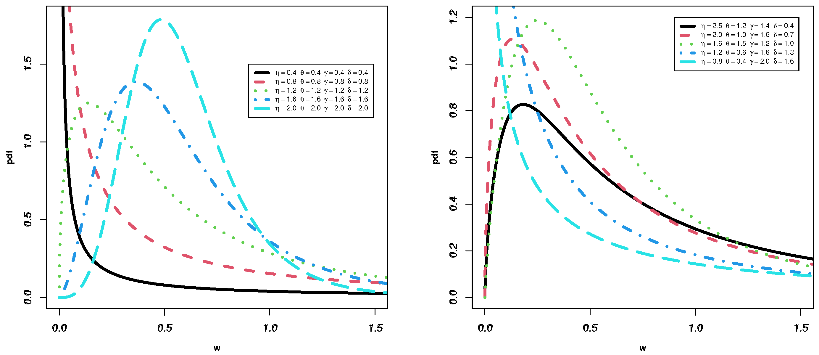
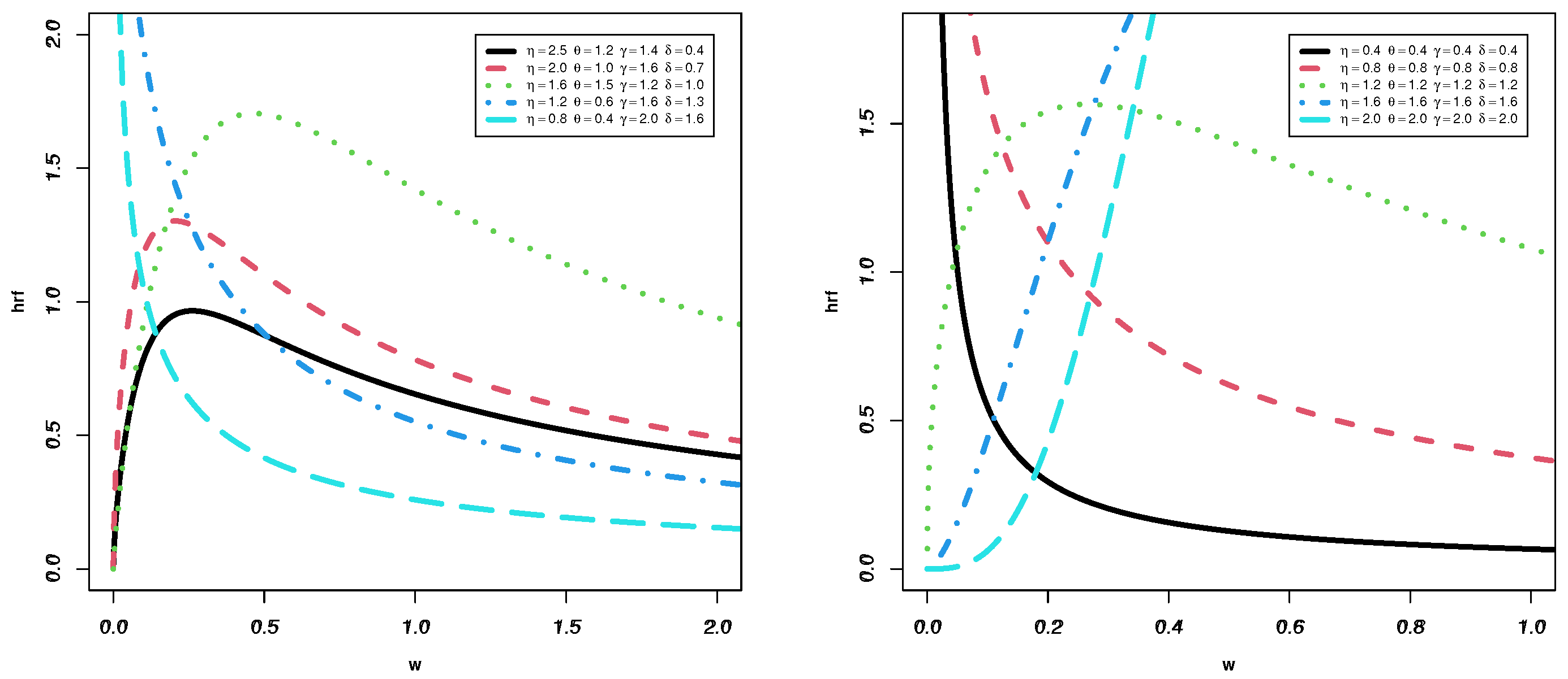
- Using the TIIEHL class of distributions to improve the properties and versatility of the PLo model (as motivated above). This assumption is shown by the observation of the uni-modal, decreasing, right skewness, and heavy-tailed forms of the pdf. The hazard rate function (hrf) can be decreasing, up-side-down, and J-shaped.
- To provide a new generalized version of the PLo model with a closed-form quantile function (QF).
- To investigate the essential statistical aspects of the TIIEHL-PLo model, such as the median, mean (), variance (var), skewness (S), kurtosis (K), raw moments, moment generating function, and order statistics.
- To investigate the statistical inference of the TIIEHL-PLo model using six different techniques of estimation such as the maximum likelihood (ML), the least square (LS) and weighted least square (WLS), maximum product spacing (MPS), Cramer-von–Mises (CVM), and the Anderson and Darling (AD) estimates.
2. Model Formulation
3. Basic Statistical Properties
3.1. Quantile Function and MacGillivray’s Skewness
3.2. Moments
3.3. Order Statistics
4. Six Different Approaches of Estimation
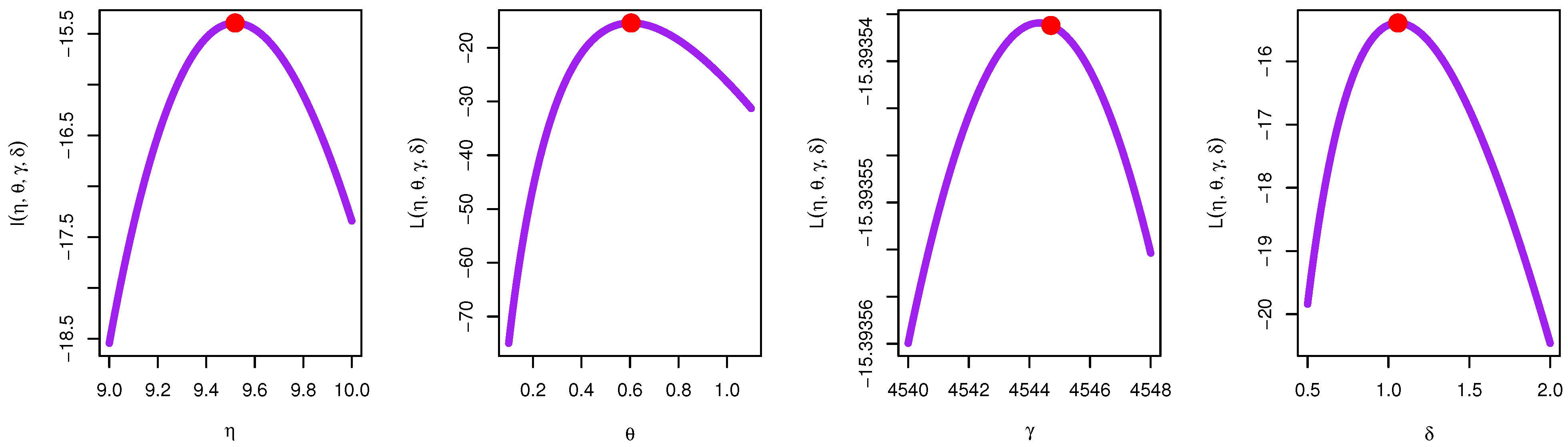
4.1. Maximum Likelihood Approach of Estimation
4.2. Maximum Product Spacing Approach of Estimation
4.3. Anderson and Darling Approach of Estimation
4.4. Cramer-von-Mises Approach of Estimation
4.5. Least Square and Weighted Least Square Approaches of Estimation
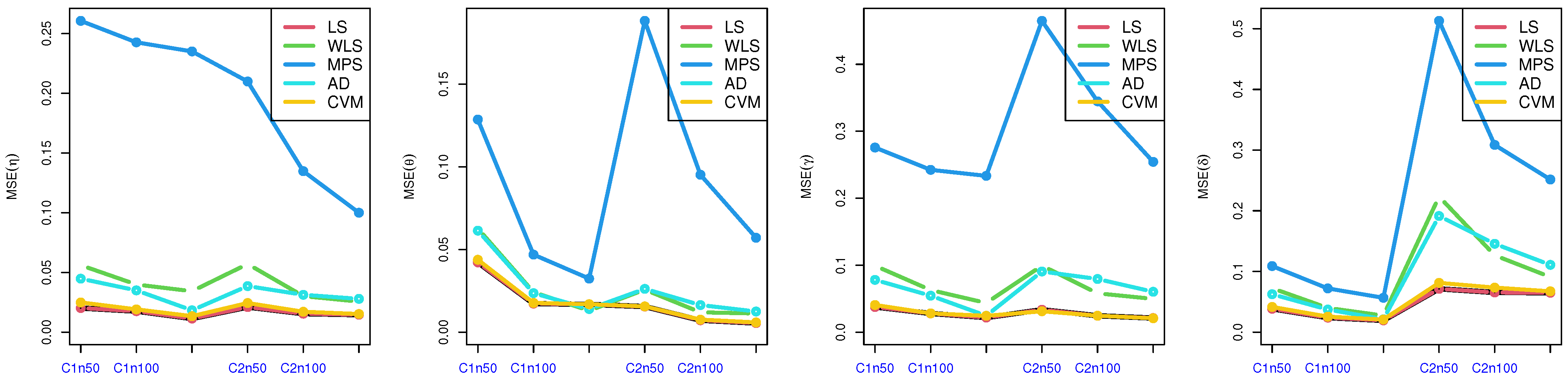
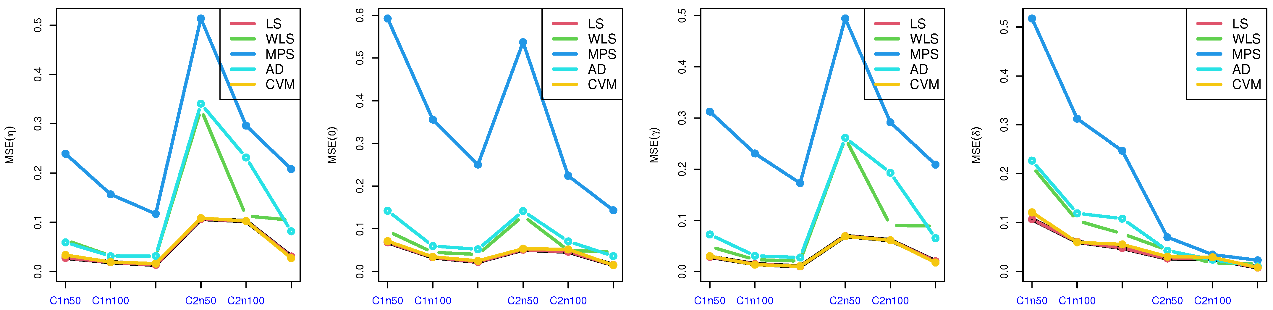
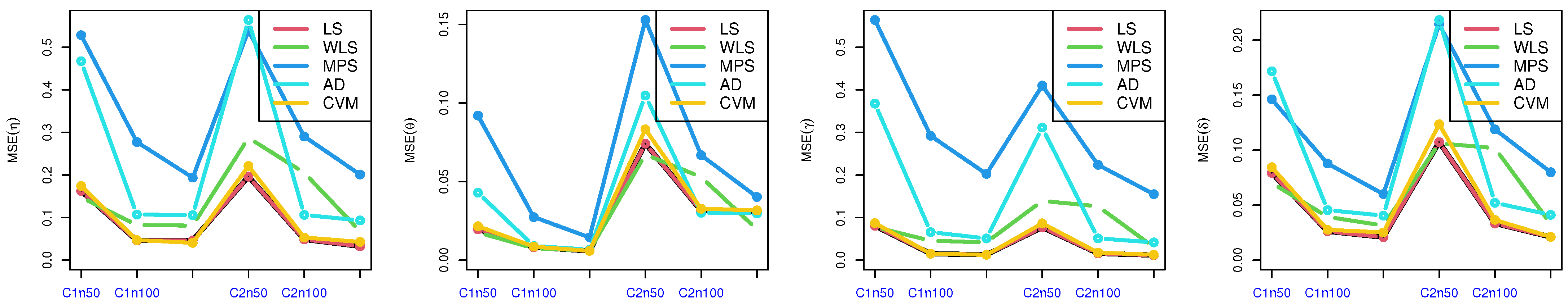
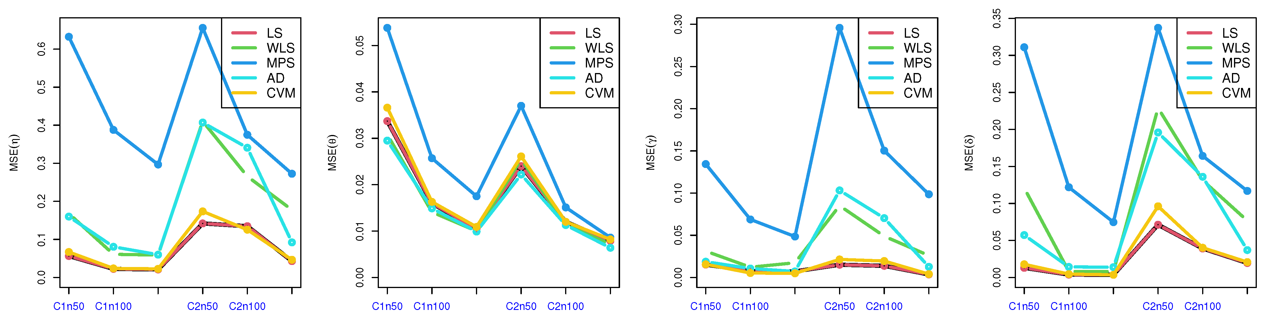
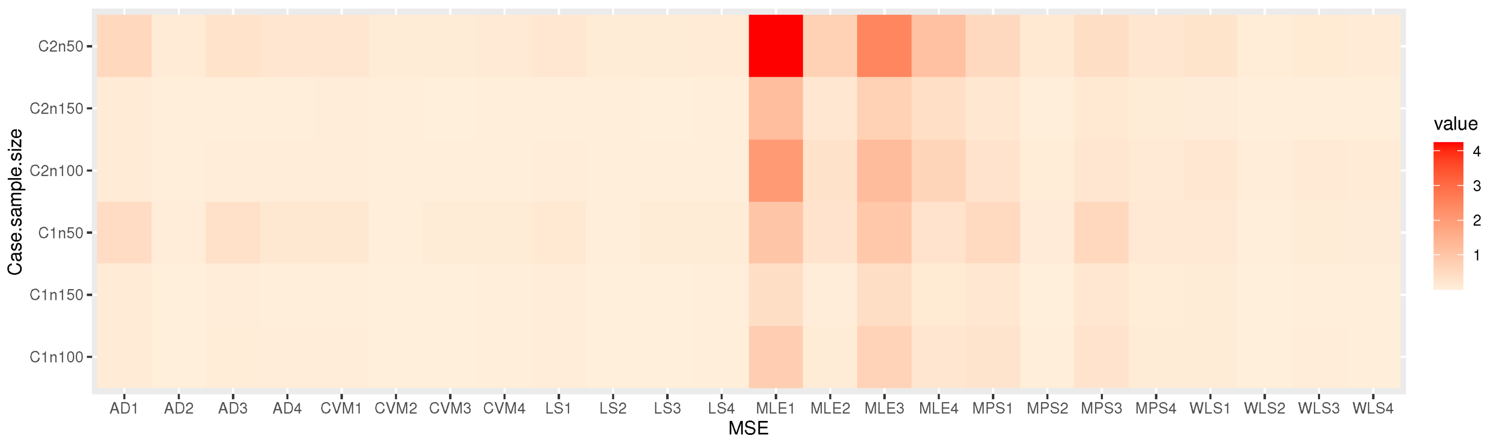
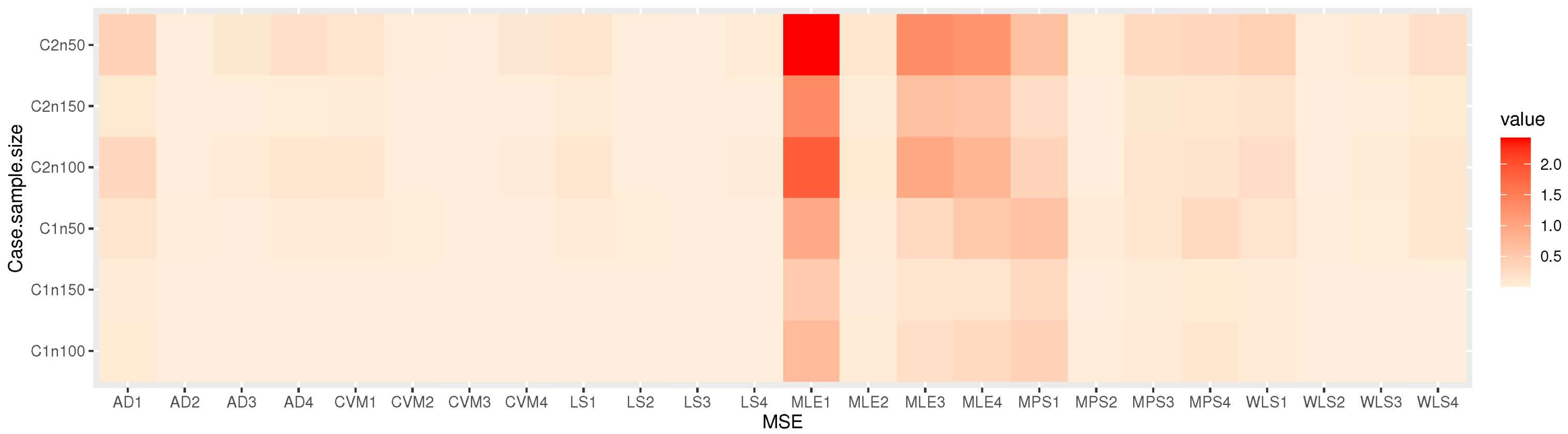
5. Simulation
- Simulation techniques for various parameters with varied actual values of the parameters, datum w is distributed as a TIIEHL-PLo distribution: Using the R package and the following:In Table 2, and 0.7, and 1.8;In Table 3, and 0.85 and 2;In Table 4, and 1.2 and 3;In Table 5, and 0.5 and 1.2.
- Set different samples sizes and 150.
- Use the numerical analysis to obtain the estimator based on different estimation methods.
- Monte Carlo trials were run using a random sample of .
- Generate a sample of the TIIEHL-PLo distribution using QF which is provided in Equation (10).
- Calculate the mean squared error (MSE) and bias of the estimator.
- The results in the tables show that the TIIEHL-PLo distribution is stable since the range of bias and MSE for the four parameters of the TIIEHL-PLo distribution is fairly modest.
- As the sample size increases, we occasionally observe a decrease in the bias and MSE for all estimations.
- This indicates that, for high sample sizes, several estimating methodologies yield a correct bias and MSE findings.
- The LS and CVM estimation approach are the most accurate means of estimating the TIIEHL-PLo distribution parameter.
- Better metrics than the MLE approaches are provided by the LS, WLS, CVM, MPS, and AD estimation methods.
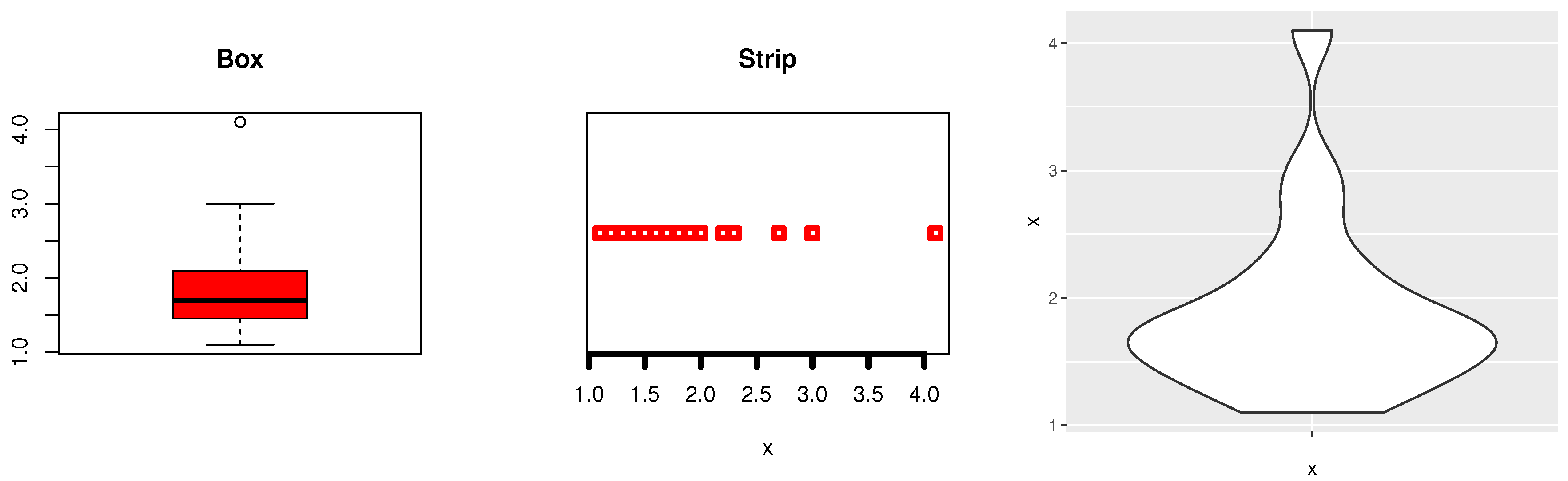
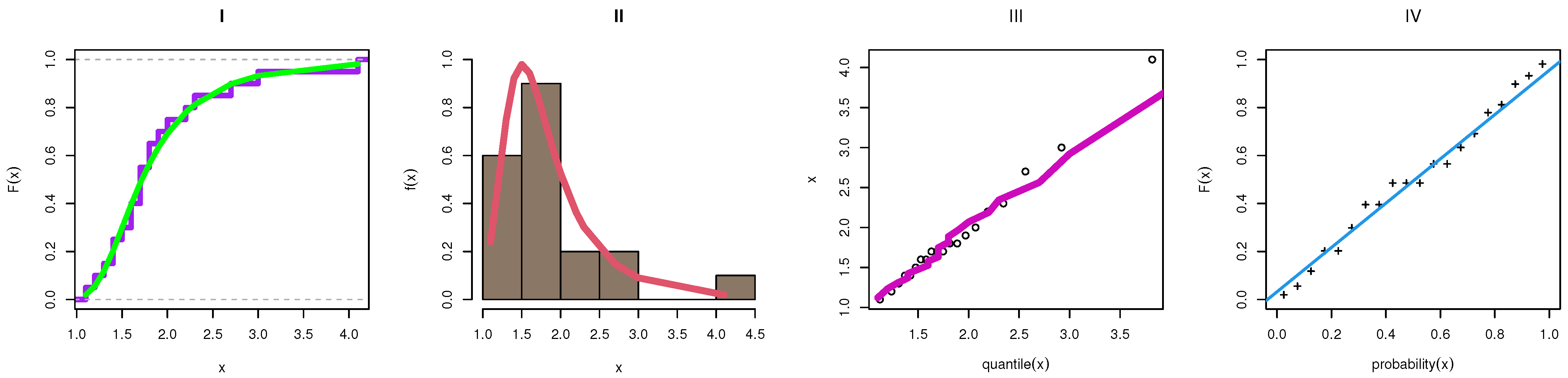
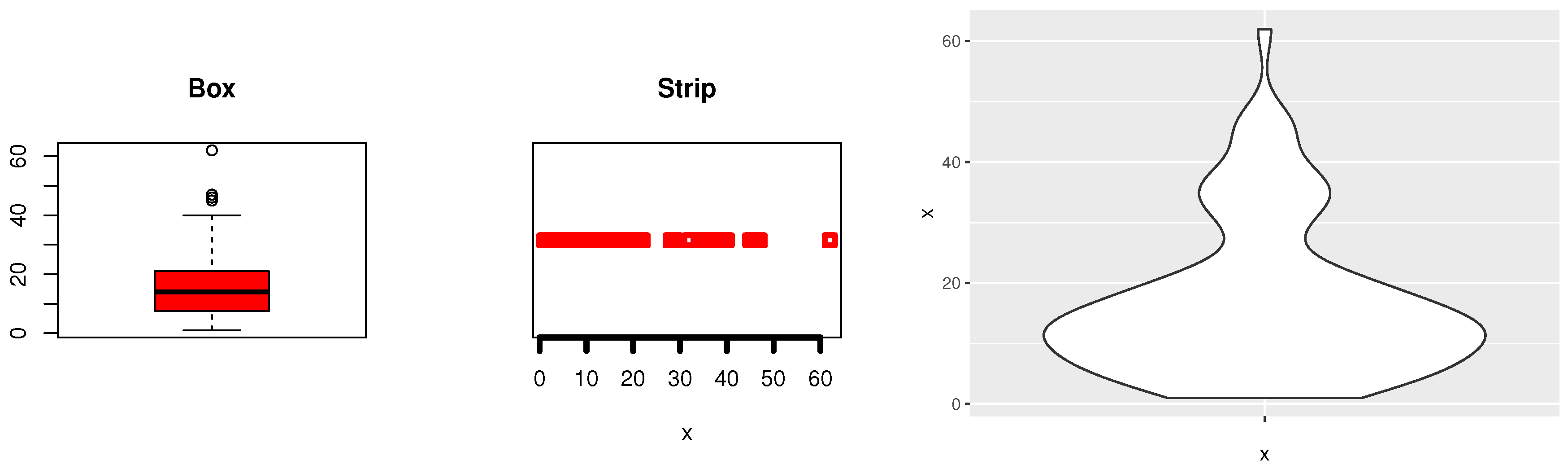
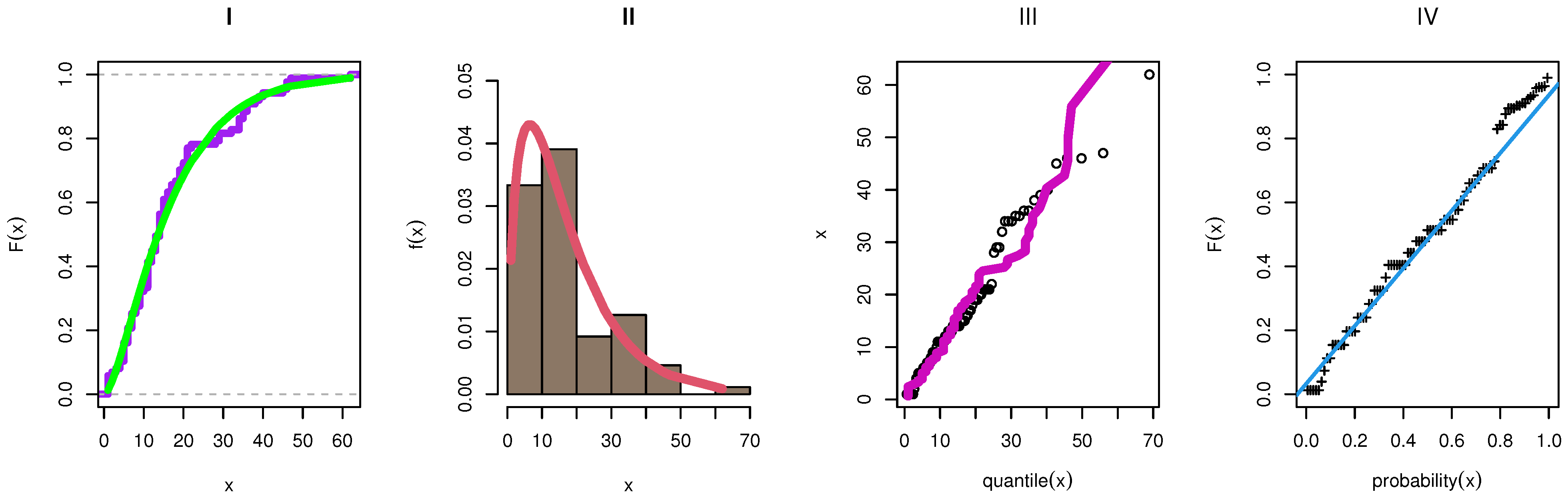
6. Modeling of Environmental and Medical Data
6.1. Environmental Data
6.2. Medical Data
7. Conclusions and Summary
Author Contributions
Funding
Data Availability Statement
Acknowledgments
Conflicts of Interest
References
- Lomax, K.S. Business failures: Another example of the analysis of failure data. J. Am. Stat. Assoc. 1954, 49, 847–852. [Google Scholar] [CrossRef]
- Hassan, A.; Al-Ghamdi, A. Optimum step stress accelerated life testing for Lomax distribution. J. Appl. Sci. Res. 2009, 5, 2153–2164. [Google Scholar]
- Atkinson, A.; Harrison, A. Distribution of Personal Wealth in Britain; Cambridge University Press: Cambridge, UK, 1978. [Google Scholar]
- Harris, C. The Pareto distribution as a queue service discipline. Oper. Res. 1968, 16, 307–313. [Google Scholar] [CrossRef]
- Chen, J.; Addie, R.G.; Zukerman, M.; Neame, T.D. Performance evaluation of a queue fed by a Poisson Lomax Burst Process. IEEE Commun. Lett. 2015, 19, 367–370. [Google Scholar] [CrossRef]
- Ghitany, M.E.; Al-Awadhi, F.A.; Alkhalfan, L.A. Marshall Olkin extended Lomax distribution and its application to censored data. Commun. Stat. Theory Methods 2007, 36, 1855–1866. [Google Scholar] [CrossRef]
- Abdul-Moniem, I.B.; Abdel-Hameed, H.F. On exponentiated Lomax distribution. Int. J. Math. Arch. 2012, 3, 2144–2150. [Google Scholar]
- Ashour, S.K.; Eltehiwy, M.A. Transmuted Lomax distribution. Am. J. Appl. Math. Stat. 2013, 1, 121–127. [Google Scholar] [CrossRef] [Green Version]
- Lemonte, A.J.; Cordeiro, G.M. An extended Lomax distribution. Statistics 2013, 47, 800–816. [Google Scholar] [CrossRef]
- Al-Zahrani, B.; Sagor, H. The Poisson-Lomax distribution. Rev. Colomb. Estad. 2014, 37, 225–245. [Google Scholar] [CrossRef]
- El-Bassiouny, A.H.; Abdo, N.F.; Shahen, H.S. Exponential Lomax distribution. Int. J. Comput. Appl. 2015, 121, 24–29. [Google Scholar]
- Cordeiro, G.M.; Ortega, E.M.; Popovíc, B.V. The gamma Lomax distribution. J. Stat. Comput. Simul. 2015, 85, 305–319. [Google Scholar] [CrossRef]
- Tahir, M.H.; Cordeiro, G.M.; Mansoor, M.; Zubair, M. The Weibull-Lomax distribution: Properties and applications. Hacet. J. Math. Stat. 2015, 44, 461–480. [Google Scholar] [CrossRef]
- Kilany, N.M. Weighted Lomax distribution. SpringerPlus 2016, 5, 1862. [Google Scholar] [CrossRef] [Green Version]
- Oguntunde, P.E.; Khaleel, M.A.; Ahmed, M.T.; Adejumo, A.O.; Odetunmibi, O.A. A New Generalization of the Lomax Distribution with Increasing, Decreasing and Constant Failure Rate. Model. Simul. Eng. 2017, 2017, 6043169. [Google Scholar] [CrossRef] [Green Version]
- Hassan, A.S.; Elgarhy, M.; Mohamed, R.E. Statistical Properties and Estimation of Type II Half Logistic Lomax Distribution. Thail. Stat. 2020, 18, 290–305. [Google Scholar]
- Tahir, M.H.; Hussain, M.A.; Cordeiro, G.M.; Hamedani, G.G.; Mansoor, M.; Zubair, M. The Gumbel-Lomax distribution: Properties and applications. J. Stat. Theory Appl. 2016, 15, 61–79. [Google Scholar] [CrossRef] [Green Version]
- Rady, E.A.; Hassanein, W.A.; Elhaddad, T.A. The power Lomax distribution with an application to bladder cancer data. SpringerPlus 2016, 5, 1838. [Google Scholar] [CrossRef] [Green Version]
- Moltok, T.T.; Dikko, H.G.; Asiribo, O.E. A transmuted Power Lomax distribution. Afr. J. Nat. Sci. 2017, 20, 67–78. [Google Scholar]
- Al-Marzouki, S. A new generalization of power Lomax distribution. Int. J. Math. Math. Sci. 2018, 7, 59–68. [Google Scholar]
- Assar, S.M. On odds generalized exponential-power Lomax distribution. J. Math. Stat. 2018, 14, 167–174. [Google Scholar] [CrossRef]
- Hassan, A.S.; Abd-Allah, M. On the inverse power Lomax distribution. Ann. Data Sci. 2019, 6, 259–278. [Google Scholar] [CrossRef]
- Al-Marzouki, S.; Jamal, F.; Chesneau, C.; Elgarhy, M. Type II Topp Leone Power Lomax Distribution with Applications. Mathematics 2020, 8, 4. [Google Scholar] [CrossRef] [Green Version]
- Algarni, A. Sine Power Lomax Model with Application to Bladder Cancer Data. Nanosci. Nanotechnol. Lett. 2020, 12, 677–684. [Google Scholar]
- Al-Mofleh, H.; Elgarhy, M.; Afify, A.Z.; Zannon, M.S. Type II exponentiated half logistic generated family of distributions with applications. Electron. J. Appl. Stat. Anal. 2020, 13, 36–561. [Google Scholar]
- Almetwally, E.M. Extended odd weibull inverse Nadarajah-Haghighi distribution with application on COVID-19 in Saudi Arabia. Math. Sci. Lett. Int. J. 2021, 10, 85–99. [Google Scholar]
- Cordeiro, G.M.; Ortega, E.M.; Nadarajah, S. The Kumaraswamy Weibull distribution with application to failure data. J. Frankl. Inst. 2010, 347, 1399–1429. [Google Scholar] [CrossRef]
- Almetwally, E.M. Marshall olkin alpha power extended Weibull distribution: Different methods of estimation based on type i and type II censoring. Gazi Univ. J. Sci. 2022, 35, 293–312. [Google Scholar]
- MacGillivray, H.L. Skewness and asymmetry: Measures and orderings. Ann. Stat. 1986, 14, 994–1011. [Google Scholar] [CrossRef]
- Macdonald, P.D.M. Comments and queries comment on “an estimation procedure for mixtures of distributions” by choi and bulgren. J. R. Stat. Soc. Ser. B (Methodol.) 1971, 33, 326–329. [Google Scholar] [CrossRef]
- Swain, J.J.; Venkatraman, S.; Wilson, J.R. Least-squares estimation of distribution functions in Johnson’s translation system. J. Stat. Comput. Simul. 1988, 29, 271–297. [Google Scholar] [CrossRef]
- Ross, M.S. Introductory Statistics, 3rd ed.; Elsevier: Oxford, UK, 2010; p. 365. [Google Scholar]
- Barco, K.V.P.; Mazucheli, J.; Janeiro, V. The inverse power Lindley distribution. Commun. Stat.-Simul. Comput. 2017, 46, 6308–6323. [Google Scholar] [CrossRef]
- Alyami, S.A.; Elbatal, I.; Alotaibi, N.; Almetwally, E.M.; Okasha, H.M.; Elgarhy, M. Topp-Leone Modified Weibull Model: Theory and Applications to Medical and Engineering Data. Appl. Sci. 2022, 12, 10431. [Google Scholar] [CrossRef]


| var | S | K | CV | ||||||||
|---|---|---|---|---|---|---|---|---|---|---|---|
| 2 | 2 | 2 | 2 | 0.6 | 0.435 | 0.383 | 0.415 | 0.076 | 1.479 | 8.287 | 0.459 |
| 2.5 | 0.654 | 0.484 | 0.404 | 0.382 | 0.056 | 1.062 | 5.82 | 0.362 | |||
| 3 | 0.696 | 0.528 | 0.435 | 0.391 | 0.044 | 0.812 | 4.806 | 0.3 | |||
| 2.5 | 2 | 0.524 | 0.327 | 0.241 | 0.211 | 0.053 | 1.245 | 6.503 | 0.438 | ||
| 2.5 | 0.587 | 0.387 | 0.284 | 0.232 | 0.042 | 0.891 | 4.92 | 0.348 | |||
| 3 | 0.637 | 0.439 | 0.327 | 0.262 | 0.034 | 0.671 | 4.234 | 0.289 | |||
| 3 | 2 | 0.471 | 0.262 | 0.17 | 0.128 | 0.04 | 1.109 | 5.673 | 0.425 | ||
| 2.5 | 0.54 | 0.325 | 0.216 | 0.158 | 0.033 | 0.788 | 4.469 | 0.338 | |||
| 3 | 0.594 | 0.38 | 0.262 | 0.193 | 0.028 | 0.584 | 3.937 | 0.282 | |||
| 3 | 2 | 2 | 0.755 | 0.657 | 0.664 | 0.799 | 0.087 | 1.479 | 8.493 | 0.39 | |
| 2.5 | 0.79 | 0.682 | 0.647 | 0.679 | 0.059 | 1.101 | 6.127 | 0.307 | |||
| 3 | 0.816 | 0.709 | 0.657 | 0.65 | 0.043 | 0.877 | 5.123 | 0.254 | |||
| 2.5 | 2 | 0.654 | 0.486 | 0.41 | 0.397 | 0.058 | 1.223 | 6.569 | 0.367 | ||
| 2.5 | 0.705 | 0.539 | 0.447 | 0.403 | 0.042 | 0.91 | 5.111 | 0.29 | |||
| 3 | 0.743 | 0.584 | 0.486 | 0.428 | 0.032 | 0.716 | 4.454 | 0.241 | |||
| 3 | 2 | 0.585 | 0.385 | 0.285 | 0.237 | 0.043 | 1.074 | 5.682 | 0.353 | ||
| 2.5 | 0.645 | 0.449 | 0.337 | 0.272 | 0.033 | 0.794 | 4.605 | 0.28 | |||
| 3 | 0.691 | 0.503 | 0.385 | 0.311 | 0.026 | 0.617 | 4.11 | 0.232 | |||
| 4 | 2 | 2 | 2 | 0.454 | 0.235 | 0.137 | 0.089 | 0.029 | 0.742 | 4.234 | 0.378 |
| 2.5 | 0.525 | 0.301 | 0.187 | 0.125 | 0.025 | 0.482 | 3.638 | 0.303 | |||
| 3 | 0.581 | 0.359 | 0.235 | 0.162 | 0.022 | 0.311 | 3.392 | 0.254 | |||
| 2.5 | 2 | 0.4 | 0.182 | 0.093 | 0.052 | 0.022 | 0.661 | 3.948 | 0.369 | ||
| 2.5 | 0.476 | 0.246 | 0.137 | 0.082 | 0.02 | 0.416 | 3.47 | 0.297 | |||
| 3 | 0.535 | 0.304 | 0.182 | 0.115 | 0.018 | 0.252 | 3.282 | 0.249 | |||
| 3 | 2 | 0.362 | 0.149 | 0.068 | 0.034 | 0.017 | 0.61 | 3.784 | 0.363 | ||
| 2.5 | 0.439 | 0.209 | 0.107 | 0.059 | 0.017 | 0.373 | 3.374 | 0.293 | |||
| 3 | 0.501 | 0.266 | 0.149 | 0.087 | 0.015 | 0.213 | 3.219 | 0.245 | |||
| 3 | 2 | 2 | 0.599 | 0.393 | 0.28 | 0.217 | 0.034 | 0.679 | 4.184 | 0.308 | |
| 2.5 | 0.659 | 0.46 | 0.34 | 0.265 | 0.026 | 0.46 | 3.696 | 0.246 | |||
| 3 | 0.703 | 0.515 | 0.393 | 0.311 | 0.021 | 0.316 | 3.485 | 0.206 | |||
| 2.5 | 2 | 0.525 | 0.3 | 0.186 | 0.124 | 0.024 | 0.584 | 3.883 | 0.297 | ||
| 2.5 | 0.593 | 0.372 | 0.246 | 0.17 | 0.02 | 0.379 | 3.513 | 0.238 | |||
| 3 | 0.645 | 0.432 | 0.3 | 0.216 | 0.017 | 0.243 | 3.361 | 0.199 | |||
| 3 | 2 | 0.474 | 0.243 | 0.134 | 0.08 | 0.019 | 0.523 | 3.713 | 0.291 | ||
| 2.5 | 0.546 | 0.315 | 0.19 | 0.12 | 0.016 | 0.326 | 3.411 | 0.233 | |||
| 3 | 0.602 | 0.376 | 0.243 | 0.163 | 0.014 | 0.195 | 3.293 | 0.195 |
| MLE | LS | WLS | MPS | CVM | AD | |||||||||
|---|---|---|---|---|---|---|---|---|---|---|---|---|---|---|
| N | Bias | MSE | Bias | MSE | Bias | MSE | Bias | MSE | Bias | MSE | Bias | MSE | ||
| 0.7 | 50 | 0.4280 | 0.7539 | 0.0622 | 0.0202 | 0.1751 | 0.0561 | 0.4285 | 0.2607 | 0.0923 | 0.0249 | 0.1623 | 0.0448 | |
| 0.0990 | 0.1072 | 0.1190 | 0.0422 | 0.1108 | 0.0627 | 0.0985 | 0.1286 | 0.1365 | 0.0438 | 0.1295 | 0.0614 | |||
| 0.3489 | 0.4889 | 0.0078 | 0.0376 | 0.1258 | 0.0992 | 0.3501 | 0.2757 | 0.0241 | 0.0406 | 0.0962 | 0.0781 | |||
| −0.0008 | 0.1380 | 0.0068 | 0.0385 | 0.0246 | 0.0724 | −0.0075 | 0.1089 | 0.0230 | 0.0416 | 0.0230 | 0.0625 | |||
| 100 | 0.5073 | 0.5146 | 0.0617 | 0.0176 | 0.1678 | 0.0399 | 0.4051 | 0.2427 | 0.0811 | 0.0191 | 0.1515 | 0.0350 | ||
| −0.0574 | 0.0439 | 0.0625 | 0.0173 | 0.0368 | 0.0242 | −0.0573 | 0.0469 | 0.0721 | 0.0177 | 0.0498 | 0.0236 | |||
| 0.3451 | 0.3547 | 0.0064 | 0.0280 | 0.1205 | 0.0629 | 0.3451 | 0.2424 | 0.0235 | 0.0281 | 0.1201 | 0.0545 | |||
| 0.0228 | 0.0901 | 0.0052 | 0.0239 | 0.0204 | 0.0399 | 0.0062 | 0.0721 | 0.0220 | 0.0256 | 0.0401 | 0.0373 | |||
| 150 | 0.4173 | 0.5023 | 0.0605 | 0.0114 | 0.1577 | 0.0343 | 0.3954 | 0.2351 | 0.0777 | 0.0134 | 0.1223 | 0.0183 | ||
| −0.0498 | 0.0325 | 0.0608 | 0.0168 | 0.0011 | 0.0130 | −0.0398 | 0.0324 | 0.0698 | 0.0169 | 0.0514 | 0.0140 | |||
| 0.4009 | 0.3238 | 0.0050 | 0.0218 | 0.1205 | 0.0436 | 0.3291 | 0.2334 | 0.0219 | 0.0244 | 0.0788 | 0.0245 | |||
| 0.0213 | 0.0790 | 0.0042 | 0.0194 | 0.0206 | 0.0273 | 0.0053 | 0.0566 | 0.0210 | 0.0208 | 0.0352 | 0.0213 | |||
| 1.8 | 50 | −0.1993 | 0.5622 | 0.0126 | 0.0210 | 0.0347 | 0.0571 | −0.1985 | 0.2099 | 0.0235 | 0.0244 | −0.0050 | 0.0386 | |
| 0.3262 | 0.1620 | 0.0296 | 0.0155 | 0.0646 | 0.0257 | 0.3264 | 0.1883 | 0.0506 | 0.0156 | 0.0613 | 0.0262 | |||
| −0.1639 | 0.6559 | −0.0198 | 0.0335 | −0.0286 | 0.0993 | −0.1640 | 0.4649 | −0.0041 | 0.0312 | −0.0192 | 0.0906 | |||
| 0.2018 | 0.8703 | 0.0010 | 0.0714 | 0.0330 | 0.2234 | 0.2009 | 0.5129 | 0.0110 | 0.0812 | 0.0636 | 0.1914 | |||
| 100 | −0.1804 | 0.2264 | 0.0126 | 0.0155 | 0.0318 | 0.0302 | −0.1807 | 0.1348 | 0.0229 | 0.0171 | 0.0154 | 0.0313 | ||
| 0.2439 | 0.0739 | 0.0200 | 0.0072 | 0.0404 | 0.0120 | 0.2441 | 0.0952 | 0.0309 | 0.0076 | 0.0608 | 0.0164 | |||
| −0.1591 | 0.3190 | −0.0154 | 0.0245 | −0.0218 | 0.0580 | −0.1592 | 0.3447 | −0.0038 | 0.0246 | −0.0336 | 0.0794 | |||
| 0.1175 | 0.3940 | −0.0010 | 0.0654 | 0.0029 | 0.1266 | 0.1173 | 0.3085 | −0.0042 | 0.0734 | 0.0106 | 0.1456 | |||
| 150 | −0.1507 | 0.2133 | 0.0123 | 0.0146 | 0.0261 | 0.0256 | −0.1509 | 0.1000 | 0.0219 | 0.0152 | 0.0242 | 0.0279 | ||
| 0.1755 | 0.0456 | 0.0166 | 0.0055 | 0.0401 | 0.0113 | 0.1755 | 0.0571 | 0.0258 | 0.0059 | 0.0530 | 0.0125 | |||
| −0.1279 | 0.3049 | −0.0092 | 0.0211 | −0.0209 | 0.0497 | −0.1280 | 0.2543 | −0.0035 | 0.0208 | −0.0285 | 0.0603 | |||
| 0.1087 | 0.3840 | 0.0002 | 0.0649 | −0.0019 | 0.0909 | 0.1089 | 0.2515 | −0.0027 | 0.0673 | −0.0059 | 0.1109 | |||
| MLE | LS | WLS | MPS | CVM | AD | |||||||||
|---|---|---|---|---|---|---|---|---|---|---|---|---|---|---|
| n | Bias | MSE | Bias | MSE | Bias | MSE | Bias | MSE | Bias | MSE | Bias | MSE | ||
| 0.85 | 50 | −0.1158 | 0.7176 | 0.0087 | 0.0276 | 0.0595 | 0.0638 | −0.1147 | 0.2391 | 0.0283 | 0.0333 | 0.0232 | 0.0591 | |
| 0.1581 | 0.5360 | 0.0052 | 0.0682 | 0.0220 | 0.0945 | 0.1583 | 0.5926 | 0.0129 | 0.0709 | 0.0414 | 0.1421 | |||
| −0.1195 | 0.6751 | −0.0015 | 0.0285 | −0.0037 | 0.0488 | −0.1194 | 0.3125 | 0.0259 | 0.0297 | −0.0106 | 0.0722 | |||
| 0.2172 | 0.9925 | 0.0480 | 0.1066 | 0.0381 | 0.2152 | 0.2162 | 0.5175 | 0.0650 | 0.1208 | 0.0718 | 0.2267 | |||
| 100 | −0.1076 | 0.4903 | 0.0067 | 0.0188 | 0.0335 | 0.0318 | −0.1078 | 0.1567 | 0.0236 | 0.0190 | 0.0346 | 0.0310 | ||
| 0.1354 | 0.3672 | 0.0052 | 0.0331 | 0.0116 | 0.0447 | 0.1356 | 0.3558 | 0.0125 | 0.0342 | 0.0226 | 0.0595 | |||
| −0.1194 | 0.4995 | −0.0015 | 0.0144 | −0.0035 | 0.0230 | −0.1196 | 0.2306 | 0.0041 | 0.0133 | −0.0089 | 0.0306 | |||
| 0.1257 | 0.5805 | −0.0157 | 0.0606 | 0.0165 | 0.1039 | 0.1255 | 0.3126 | 0.0053 | 0.0596 | 0.0135 | 0.1189 | |||
| 150 | −0.0927 | 0.3670 | 0.0061 | 0.0133 | 0.0327 | 0.0306 | −0.0930 | 0.1169 | 0.0238 | 0.0159 | 0.0331 | 0.0314 | ||
| 0.1061 | 0.2978 | −0.0005 | 0.0224 | 0.0102 | 0.0398 | 0.1061 | 0.2503 | 0.0065 | 0.0248 | 0.0199 | 0.0518 | |||
| −0.0981 | 0.4457 | 0.0012 | 0.0097 | −0.0034 | 0.0201 | −0.0982 | 0.1726 | 0.0041 | 0.0101 | −0.0050 | 0.0271 | |||
| 0.1078 | 0.4370 | 0.0148 | 0.0479 | −0.0135 | 0.0773 | 0.1081 | 0.2468 | 0.0042 | 0.0554 | 0.0125 | 0.1080 | |||
| 2 | 50 | −0.0369 | 2.5221 | −0.0068 | 0.1066 | 0.0114 | 0.3297 | −0.0363 | 0.5137 | 0.0058 | 0.1083 | 0.0085 | 0.3407 | |
| 0.1304 | 0.9183 | 0.0100 | 0.0510 | 0.0363 | 0.1301 | 0.1302 | 0.5371 | 0.0265 | 0.0533 | 0.0477 | 0.1415 | |||
| −0.0608 | 1.8920 | −0.0055 | 0.0692 | 0.0154 | 0.2606 | −0.0601 | 0.4946 | 0.0088 | 0.0687 | 0.0133 | 0.2614 | |||
| −0.0278 | 0.2960 | 0.0077 | 0.0264 | 0.0064 | 0.0438 | −0.0283 | 0.0700 | 0.0282 | 0.0302 | 0.0149 | 0.0426 | |||
| 100 | −0.0301 | 1.8807 | 0.0061 | 0.1023 | −0.0037 | 0.1128 | −0.0300 | 0.2962 | 0.0042 | 0.1025 | 0.0073 | 0.2314 | ||
| 0.0616 | 0.5196 | 0.0100 | 0.0461 | 0.0152 | 0.0494 | 0.0615 | 0.2241 | 0.0197 | 0.0516 | 0.0146 | 0.0704 | |||
| −0.0330 | 1.4274 | 0.0055 | 0.0611 | −0.0047 | 0.0900 | −0.0328 | 0.2915 | 0.0069 | 0.0609 | 0.0132 | 0.1928 | |||
| −0.0131 | 0.1896 | 0.0035 | 0.0257 | 0.0032 | 0.0163 | −0.0131 | 0.0344 | 0.0101 | 0.0289 | −0.0011 | 0.0239 | |||
| 150 | −0.0362 | 1.1643 | −0.0001 | 0.0304 | 0.0037 | 0.1040 | −0.0301 | 0.2080 | 0.0038 | 0.0271 | −0.0034 | 0.0815 | ||
| 0.0562 | 0.3912 | 0.0020 | 0.0153 | 0.0120 | 0.0455 | 0.0563 | 0.1433 | 0.0074 | 0.0147 | 0.0137 | 0.0360 | |||
| −0.0445 | 0.8100 | −0.0001 | 0.0200 | 0.0038 | 0.0886 | −0.0304 | 0.2089 | 0.0040 | 0.0174 | −0.0033 | 0.0652 | |||
| −0.0085 | 0.1514 | 0.0021 | 0.0080 | 0.0014 | 0.0158 | −0.0082 | 0.0228 | 0.0084 | 0.0082 | 0.0058 | 0.0103 | |||
| MLE | LS | WLS | MPS | CVM | AD | |||||||||
|---|---|---|---|---|---|---|---|---|---|---|---|---|---|---|
| n | Bias | MSE | Bias | MSE | Bias | MSE | Bias | MSE | Bias | MSE | Bias | MSE | ||
| 1.2 | 50 | −0.0334 | 1.0185 | 0.0070 | 0.1627 | −0.0056 | 0.1478 | −0.0330 | 0.5284 | 0.0233 | 0.1741 | 0.0018 | 0.4672 | |
| 0.0557 | 0.2945 | 0.0045 | 0.0196 | 0.0137 | 0.0176 | 0.0556 | 0.0920 | 0.0290 | 0.0216 | 0.0515 | 0.0429 | |||
| −0.0531 | 0.9668 | −0.0073 | 0.0806 | −0.0128 | 0.0780 | −0.0527 | 0.5641 | 0.0037 | 0.0868 | −0.0244 | 0.3677 | |||
| −0.0123 | 0.2988 | 0.0049 | 0.0793 | 0.0187 | 0.0701 | −0.0127 | 0.1462 | 0.0190 | 0.0845 | 0.0293 | 0.1717 | |||
| 100 | −0.0118 | 0.8033 | −0.0051 | 0.0462 | 0.0043 | 0.0824 | −0.0117 | 0.2774 | 0.0021 | 0.0472 | 0.0016 | 0.1072 | ||
| 0.0146 | 0.0913 | −0.0014 | 0.0082 | 0.0036 | 0.0076 | 0.0146 | 0.0274 | 0.0107 | 0.0086 | 0.0080 | 0.0090 | |||
| −0.0212 | 0.6897 | −0.0047 | 0.0151 | −0.0066 | 0.0455 | −0.0210 | 0.2920 | −0.0048 | 0.0153 | −0.0032 | 0.0658 | |||
| −0.0170 | 0.2239 | 0.0051 | 0.0262 | 0.0022 | 0.0393 | −0.0117 | 0.0878 | 0.0149 | 0.0276 | 0.0062 | 0.0455 | |||
| 150 | −0.0145 | 0.4159 | 0.0048 | 0.0465 | −0.0022 | 0.0811 | −0.0105 | 0.1938 | 0.0022 | 0.0406 | 0.0016 | 0.1058 | ||
| 0.0134 | 0.0465 | −0.0002 | 0.0059 | 0.0022 | 0.0061 | 0.0134 | 0.0145 | 0.0073 | 0.0059 | 0.0078 | 0.0067 | |||
| −0.0240 | 0.4163 | 0.0047 | 0.0129 | −0.0062 | 0.0419 | −0.0204 | 0.2024 | 0.0044 | 0.0125 | 0.0030 | 0.0510 | |||
| −0.0067 | 0.1389 | −0.0040 | 0.0209 | 0.0025 | 0.0315 | −0.0066 | 0.0601 | 0.0031 | 0.0252 | −0.0042 | 0.0405 | |||
| 3 | 50 | −0.0243 | 4.2460 | −0.0017 | 0.1962 | 0.0130 | 0.2873 | −0.0240 | 0.5391 | 0.0148 | 0.2211 | 0.0231 | 0.5641 | |
| 0.0165 | 0.7345 | 0.0035 | 0.0741 | 0.0072 | 0.0672 | 0.0164 | 0.1528 | 0.0228 | 0.0832 | 0.0255 | 0.1047 | |||
| −0.0359 | 2.4839 | −0.0074 | 0.0770 | 0.0038 | 0.1393 | −0.0355 | 0.4100 | 0.0020 | 0.0865 | 0.0038 | 0.3113 | |||
| 0.0015 | 1.1197 | 0.0138 | 0.1073 | 0.0089 | 0.1062 | 0.0011 | 0.2145 | 0.0379 | 0.1235 | 0.0272 | 0.2183 | |||
| 100 | −0.0069 | 2.0304 | −0.0010 | 0.0488 | 0.0128 | 0.2052 | −0.0068 | 0.2905 | 0.0062 | 0.0532 | 0.0107 | 0.1062 | ||
| 0.0012 | 0.3298 | −0.0027 | 0.0315 | 0.0061 | 0.0529 | 0.0011 | 0.0668 | 0.0070 | 0.0327 | 0.0032 | 0.0301 | |||
| −0.0138 | 1.2379 | −0.0027 | 0.0159 | 0.0021 | 0.1264 | −0.0136 | 0.2238 | 0.0012 | 0.0177 | 0.0037 | 0.0511 | |||
| −0.0118 | 0.6388 | 0.0007 | 0.0334 | 0.0064 | 0.1018 | −0.0012 | 0.1189 | 0.0129 | 0.0366 | 0.0010 | 0.0521 | |||
| 150 | −0.0126 | 1.1938 | 0.0012 | 0.0326 | 0.0068 | 0.0678 | −0.0061 | 0.2011 | 0.0052 | 0.0429 | 0.0107 | 0.0933 | ||
| 0.0048 | 0.1946 | 0.0027 | 0.0306 | 0.0027 | 0.0196 | 0.0010 | 0.0402 | 0.0061 | 0.0317 | 0.0031 | 0.0298 | |||
| −0.0187 | 0.7477 | 0.0007 | 0.0118 | 0.0021 | 0.0305 | −0.0129 | 0.1549 | 0.0011 | 0.0127 | 0.0031 | 0.0417 | |||
| −0.0016 | 0.4042 | 0.0007 | 0.0211 | 0.0026 | 0.0329 | −0.0010 | 0.0799 | 0.0111 | 0.0212 | 0.0010 | 0.0412 | |||
| MLE | LS | WLS | MPS | CVM | AD | |||||||||
|---|---|---|---|---|---|---|---|---|---|---|---|---|---|---|
| n | Bias | MSE | Bias | MSE | Bias | MSE | Bias | MSE | Bias | MSE | Bias | MSE | ||
| 0.5 | 50 | −0.1133 | 0.9396 | −0.0092 | 0.0564 | −0.0283 | 0.1679 | −0.1130 | 0.6324 | −0.0084 | 0.0669 | −0.0374 | 0.1600 | |
| −0.0529 | 0.0728 | −0.0084 | 0.0337 | −0.0097 | 0.0308 | −0.0526 | 0.0538 | 0.0209 | 0.0366 | −0.0066 | 0.0295 | |||
| −0.0320 | 0.3072 | 0.0068 | 0.0153 | 0.0043 | 0.0312 | −0.0319 | 0.1344 | 0.0108 | 0.0156 | 0.0048 | 0.0187 | |||
| 0.4889 | 0.5335 | 0.0404 | 0.0130 | 0.1409 | 0.1209 | 0.4879 | 0.3110 | 0.0472 | 0.0178 | 0.1406 | 0.0573 | |||
| 100 | −0.0755 | 0.7256 | −0.0004 | 0.0226 | −0.0056 | 0.0609 | −0.0754 | 0.3877 | −0.0023 | 0.0238 | −0.0134 | 0.0806 | ||
| −0.0343 | 0.0511 | −0.0052 | 0.0160 | −0.0036 | 0.0141 | −0.0342 | 0.0257 | 0.0090 | 0.0163 | −0.0043 | 0.0149 | |||
| −0.0263 | 0.2340 | 0.0023 | 0.0074 | 0.0037 | 0.0122 | −0.0264 | 0.0688 | 0.0030 | 0.0053 | 0.0030 | 0.0106 | |||
| 0.2619 | 0.2949 | 0.0121 | 0.0039 | 0.0319 | 0.0081 | 0.2615 | 0.1219 | 0.0164 | 0.0046 | 0.0530 | 0.0143 | |||
| 150 | −0.0736 | 0.5195 | −0.0003 | 0.0211 | −0.0041 | 0.0589 | −0.0736 | 0.2968 | 0.0001 | 0.0226 | −0.0124 | 0.0599 | ||
| −0.0258 | 0.0391 | −0.0027 | 0.0105 | −0.0027 | 0.0100 | −0.0257 | 0.0175 | 0.0074 | 0.0109 | −0.0019 | 0.0099 | |||
| −0.0261 | 0.1483 | 0.0023 | 0.0072 | 0.0013 | 0.0174 | −0.0262 | 0.0485 | 0.0030 | 0.0049 | 0.0005 | 0.0072 | |||
| 0.2072 | 0.1649 | 0.0119 | 0.0036 | 0.0347 | 0.0081 | 0.2071 | 0.0747 | 0.0116 | 0.0036 | 0.0470 | 0.0139 | |||
| 1.2 | 50 | −0.0437 | 2.4249 | −0.0144 | 0.1420 | −0.0140 | 0.4104 | −0.0431 | 0.6558 | −0.0120 | 0.1736 | 0.0030 | 0.4071 | |
| −0.0055 | 0.1348 | −0.0074 | 0.0240 | 0.0009 | 0.0255 | −0.0054 | 0.0370 | 0.0162 | 0.0261 | 0.0073 | 0.0222 | |||
| −0.0305 | 1.3166 | −0.0022 | 0.0151 | −0.0042 | 0.0851 | −0.0302 | 0.2958 | −0.0006 | 0.0214 | 0.0050 | 0.1032 | |||
| 0.1500 | 1.2372 | 0.0541 | 0.0713 | 0.1227 | 0.2290 | 0.1493 | 0.3372 | 0.0824 | 0.0962 | 0.0997 | 0.1959 | |||
| 100 | −0.0215 | 1.8760 | 0.0102 | 0.1348 | −0.0125 | 0.2657 | −0.0214 | 0.3749 | 0.0123 | 0.1255 | 0.0030 | 0.3408 | ||
| −0.0101 | 0.0870 | −0.0041 | 0.0120 | −0.0008 | 0.0113 | −0.0041 | 0.0151 | 0.0078 | 0.0120 | −0.0003 | 0.0113 | |||
| −0.0157 | 0.9802 | 0.0019 | 0.0138 | −0.0010 | 0.0489 | −0.0156 | 0.1503 | 0.0006 | 0.0195 | 0.0050 | 0.0703 | |||
| 0.0770 | 0.7863 | −0.0062 | 0.0392 | 0.0849 | 0.1312 | 0.0768 | 0.1642 | 0.0079 | 0.0402 | 0.0649 | 0.1360 | |||
| 150 | −0.0283 | 1.3563 | −0.0066 | 0.0431 | 0.0024 | 0.1775 | −0.0208 | 0.2725 | −0.0020 | 0.0465 | 0.0019 | 0.0922 | ||
| −0.0048 | 0.0442 | −0.0027 | 0.0079 | −0.0004 | 0.0072 | −0.0040 | 0.0086 | 0.0055 | 0.0082 | 0.0002 | 0.0064 | |||
| −0.0209 | 0.6381 | −0.0012 | 0.0036 | 0.0010 | 0.0260 | −0.0121 | 0.0986 | 0.0004 | 0.0040 | 0.0015 | 0.0127 | |||
| 0.0702 | 0.5834 | 0.0052 | 0.0196 | 0.0448 | 0.0767 | 0.0703 | 0.1169 | 0.0062 | 0.0208 | 0.0236 | 0.0370 | |||
| MLE | LS | WLS | MPS | CVM | AD | ||
|---|---|---|---|---|---|---|---|
| n | |||||||
| 0.7 | 50 | 0.3720 | 0.0346 | 0.0726 | 0.1935 | 0.0377 | 0.0617 |
| 100 | 0.2508 | 0.0217 | 0.0417 | 0.1510 | 0.0226 | 0.0376 | |
| 150 | 0.2344 | 0.0173 | 0.0296 | 0.1394 | 0.0189 | 0.0195 | |
| 1.8 | 50 | 0.5626 | 0.0353 | 0.1014 | 0.3440 | 0.0381 | 0.0867 |
| 100 | 0.2533 | 0.0281 | 0.0567 | 0.2208 | 0.0307 | 0.0682 | |
| 150 | 0.2370 | 0.0265 | 0.0444 | 0.1657 | 0.0273 | 0.0529 | |
| n | |||||||
| 0.85 | 50 | 0.7303 | 0.0577 | 0.1056 | 0.4154 | 0.0637 | 0.1250 |
| 100 | 0.4844 | 0.0317 | 0.0508 | 0.2639 | 0.0315 | 0.0600 | |
| 150 | 0.3869 | 0.0233 | 0.0419 | 0.1967 | 0.0265 | 0.0546 | |
| 2 | 50 | 1.4071 | 0.0633 | 0.1910 | 0.4039 | 0.0651 | 0.1965 |
| 100 | 1.0043 | 0.0588 | 0.0671 | 0.2116 | 0.0610 | 0.1296 | |
| 150 | 0.6292 | 0.0184 | 0.0635 | 0.1457 | 0.0168 | 0.0482 | |
| n | |||||||
| 1.2 | 50 | 0.6446 | 0.0855 | 0.0784 | 0.3327 | 0.0917 | 0.2624 |
| 100 | 0.4521 | 0.0239 | 0.0437 | 0.1711 | 0.0247 | 0.0569 | |
| 150 | 0.2544 | 0.0216 | 0.0401 | 0.1177 | 0.0211 | 0.0510 | |
| 3 | 50 | 2.1460 | 0.1137 | 0.1500 | 0.3291 | 0.1286 | 0.2996 |
| 100 | 1.0592 | 0.0324 | 0.1216 | 0.1750 | 0.0351 | 0.0599 | |
| 150 | 0.6351 | 0.0240 | 0.0377 | 0.1190 | 0.0271 | 0.0515 | |
| n | |||||||
| 0.5 | 50 | 0.4633 | 0.0296 | 0.0877 | 0.2829 | 0.0342 | 0.0664 |
| 100 | 0.3264 | 0.0125 | 0.0238 | 0.1510 | 0.0125 | 0.0301 | |
| 150 | 0.2179 | 0.0106 | 0.0236 | 0.1094 | 0.0105 | 0.0227 | |
| 1.2 | 50 | 1.2784 | 0.0631 | 0.1875 | 0.3315 | 0.0793 | 0.1821 |
| 100 | 0.9324 | 0.0500 | 0.1143 | 0.1762 | 0.0493 | 0.1396 | |
| 150 | 0.6555 | 0.0185 | 0.0718 | 0.1242 | 0.0199 | 0.0370 | |
| Models | Estimates | SE | CVM | AD | KS | PVKS | |||||
|---|---|---|---|---|---|---|---|---|---|---|---|
| TIIEHL-PLo | 0.0547 | 0.0025 | 101.4707 | 108.2262 | 102.6136 | 103.9133 | 0.0423 | 0.3147 | 0.0764 | 0.9738 | |
| 11.9313 | 6.5648 | ||||||||||
| 10.2097 | 5.2268 | ||||||||||
| 120.4763 | 26.4693 | ||||||||||
| EOWINH | 7.7423 | 2.4349 | 102.4427 | 103.5855 | 109.1982 | 104.8853 | 0.0427 | 0.3298 | 0.0809 | 0.9560 | |
| 0.4600 | 0.5247 | ||||||||||
| 0.9827 | 0.9747 | ||||||||||
| 5.7681 | 4.7740 | ||||||||||
| KW | 0.1322 | 0.0142 | 99.2020 | 100.3448 | 105.9575 | 101.6446 | 0.0255 | 0.2087 | 0.0656 | 0.9954 | |
| 3.3827 | 0.0097 | ||||||||||
| 13.7096 | 0.5152 | ||||||||||
| 0.1023 | 0.0214 | ||||||||||
| MOAPLo | 294.3313 | 21.2626 | 105.5206 | 106.6635 | 112.2761 | 107.9632 | 0.0698 | 0.4915 | 0.0828 | 0.9469 | |
| 27.7774 | 23.9966 | ||||||||||
| 1180.6838 | 39.5466 | ||||||||||
| 9.5382 | 9.3425 | ||||||||||
| MOAPEW | 54.5650 | 140.1735 | 107.1567 | 108.9214 | 115.6011 | 110.2099 | 0.0791 | 0.5424 | 0.0808 | 0.9567 | |
| 2.9115 | 2.1861 | ||||||||||
| 0.8447 | 2.3056 | ||||||||||
| 24.1657 | 112.4007 | ||||||||||
| 17.6442 | 118.2467 | ||||||||||
| ELo | 137.985746 | 112.6857 | 101.3571 | 108.80238 | 105.42374 | 104.18904 | 0.043415 | 0.336339 | 0.085706 | 0.930577 | |
| 75.35675 | 219.6866 | ||||||||||
| 47.6452043 | 149.0872 | ||||||||||
| IWLoPS | 0.0540 | 0.0301 | 101.9895 | 103.1323 | 108.7450 | 104.4321 | 0.0479 | 0.3487 | 0.0773 | 0.9706 | |
| 345.6694 | 190.0276 | ||||||||||
| 99.8438 | 52.5460 | ||||||||||
| 1.2466 | 0.9456 | ||||||||||
| WLo | 1.6850 | 3.6630 | 103.5711 | 104.7139 | 110.3266 | 106.0137 | 0.0771 | 0.5231 | 0.0947 | 0.8655 | |
| 10.3668 | 9.1686 | ||||||||||
| 0.2485 | 0.2101 | ||||||||||
| 0.2855 | 0.9960 | ||||||||||
| GLo | 103.5638 | 357.9515 | 102.2910 | 103.4338 | 109.0465 | 104.7335 | 0.0431 | 0.3341 | 0.0852 | 0.9334 | |
| 73.8117 | 277.9995 | ||||||||||
| 0.9181 | 1.7041 | ||||||||||
| 122.1513 | 132.8174 |
| MLE | LS | WLS | MPS | CVM | AD | |
|---|---|---|---|---|---|---|
| 0.0547 | 0.0357 | 0.0665 | 0.0500 | 0.0414 | 0.0436 | |
| 11.9313 | 17.1084 | 9.0774 | 11.7787 | 12.8477 | 13.4472 | |
| 10.2097 | 8.9407 | 8.9112 | 9.1147 | 8.2366 | 8.9022 | |
| 120.4763 | 88.0345 | 92.3735 | 120.8870 | 123.9244 | 109.8484 | |
| KS | 0.0764 | 0.0563 | 0.0558 | 0.0611 | 0.0603 | 0.0582 |
| PVKS | 0.9738 | 0.9996 | 0.9996 | 0.9983 | 0.9986 | 0.9993 |
| Models | Estimates | SE | CVM | AD | KS | PVKS | |||||
|---|---|---|---|---|---|---|---|---|---|---|---|
| TIIEHL-PLo | 9.5189 | 2.5157 | 38.7871 | 42.7700 | 41.4538 | 39.5646 | 0.0266 | 0.1515 | 0.0952 | 0.9935 | |
| 0.6046 | 0.5165 | ||||||||||
| 4544.7074 | 25.5165 | ||||||||||
| 1.0583 | 0.8994 | ||||||||||
| EOWINH | 146.9404 | 1.3401 | 43.2241 | 45.8908 | 47.2070 | 44.0016 | 0.0971 | 0.5746 | 0.1686 | 0.6202 | |
| 5.0325 | 0.1032 | ||||||||||
| 10.7858 | 1.0159 | ||||||||||
| 0.8082 | 1.3055 | ||||||||||
| KW | 2.1289 | 0.7607 | 41.1433 | 43.8099 | 45.1262 | 41.9208 | 0.0627 | 0.3691 | 0.1488 | 0.7679 | |
| 0.8551 | 0.3273 | ||||||||||
| 28.9148 | 24.2893 | ||||||||||
| 1.2803 | 1.1606 | ||||||||||
| MOAPLo | 546,390.9153 | 225.1516 | 44.8576 | 47.5243 | 48.8405 | 45.6351 | 0.1168 | 0.6871 | 0.1290 | 0.8931 | |
| 1,287,898.0703 | 2356.5153 | ||||||||||
| 8.6949 | 3.1731 | ||||||||||
| 475,204.4105 | 130.0856 | ||||||||||
| MOAPEW | 38.8928 | 41.7939 | 48.5882 | 52.8739 | 53.5669 | 49.5601 | 0.1341 | 0.7925 | 0.1517 | 0.7467 | |
| 2.5248 | 0.6696 | ||||||||||
| 0.1090 | 0.1214 | ||||||||||
| 32.1868 | 12.1517 | ||||||||||
| 25.2059 | 34.5792 | ||||||||||
| ELo | 77.2175 | 116.8405 | 39.1512 | 43.0124 | 41.9955 | 39.9549 | 0.0391 | 0.2260 | 0.1211 | 0.9308 | |
| 12.0930 | 17.6372 | ||||||||||
| 3.6927 | 7.7470 | ||||||||||
| IWLoPS | 1.3286 | 5.8583 | 38.8502 | 42.8152 | 42.8331 | 39.6277 | 0.0253 | 0.1457 | 0.0945 | 0.9941 | |
| 3.0159 | 8.0370 | ||||||||||
| 11.6474 | 59.2088 | ||||||||||
| 1.0065 | 1.5240 | ||||||||||
| WLo | 8.3496 | 34.5554 | 47.3153 | 49.9820 | 51.2982 | 48.0928 | 0.1575 | 0.9298 | 0.1790 | 0.5430 | |
| 5.6433 | 4.1698 | ||||||||||
| 0.2286 | 0.2052 | ||||||||||
| 0.2380 | 0.6492 | ||||||||||
| GLo | 1.6185 | 4.0536 | 38.7894 | 42.8456 | 42.7723 | 39.5669 | 0.0285 | 0.1610 | 0.0961 | 0.9926 | |
| 1.1993 | 0.5152 | ||||||||||
| 0.3103 | 0.3337 | ||||||||||
| 30.0251 | 8.2652 |
| MLE | LS | WLS | MPS | CVM | AD | |
|---|---|---|---|---|---|---|
| 9.5189 | 9.9205 | 9.7301 | 11.1211 | 9.4695 | 9.5634 | |
| 0.6046 | 0.5250 | 0.5259 | 0.7125 | 0.5733 | 0.5682 | |
| 4544.7074 | 5552.7217 | 4547.8144 | 4602.8831 | 4548.3921 | 4544.2005 | |
| 1.0583 | 1.1914 | 1.1224 | 0.1279 | 1.2596 | 1.1490 | |
| KS | 0.0952 | 0.0945 | 0.1011 | 0.4691 | 0.0890 | 0.0941 |
| PVKS | 0.9935 | 0.9943 | 0.9868 | 0.0003 | 0.9974 | 0.9944 |
| Models | Estimates | SE | CVM | AD | KS | PVKS | |||||
|---|---|---|---|---|---|---|---|---|---|---|---|
| TIIEHL-PLo | 1.8085 | 1.2965 | 664.2789 | 674.1425 | 664.7667 | 668.2506 | 0.0817 | 0.6012 | 0.0710 | 0.7725 | |
| 0.1161 | 0.0952 | ||||||||||
| 41.3607 | 21.2156 | ||||||||||
| 6812.653 | 178.7555 | ||||||||||
| EOWINH | 143.3842 | 51.2157 | 669.3280 | 679.8158 | 679.1916 | 673.2997 | 0.1287 | 1.0204 | 0.1241 | 0.1370 | |
| 133.7293 | 303.9769 | ||||||||||
| 33.8102 | 20.1257 | ||||||||||
| 0.4976 | 0.3460 | ||||||||||
| KW | 0.0808 | 0.2125 | 664.8686 | 674.3564 | 673.7322 | 669.8404 | 0.0911 | 0.6100 | 0.0739 | 0.7284 | |
| 1.2726 | 0.2508 | ||||||||||
| 1.1680 | 0.5009 | ||||||||||
| 0.3210 | 0.9742 | ||||||||||
| MOAPLo | 0.0269 | 0.0419 | 664.3716 | 674.5594 | 673.9352 | 668.4334 | 0.0823 | 0.6184 | 0.0731 | 0.7413 | |
| 90.5058 | 30.9432 | ||||||||||
| 15.1273 | 11.1261 | ||||||||||
| 1104.807 | 861.105 | ||||||||||
| MOAPEW | 5.4995 | 6.7764 | 673.4946 | 674.9235 | 685.8242 | 678.4593 | 0.2217 | 1.2727 | 0.0914 | 0.4609 | |
| 0.2972 | 0.1458 | ||||||||||
| 5.1496 | 11.4986 | ||||||||||
| 1.5716 | 4.0306 | ||||||||||
| 0.2669 | 0.5105 | ||||||||||
| ELo | 1.812536 | 0.316325 | 665.7241 | 674.2132 | 671.1218 | 669.7029 | 0.086053 | 0.618995 | 0.084499 | 0.563524 | |
| 11.24635 | 8.116818 | ||||||||||
| 123.1732 | 102.2685 | ||||||||||
| IWLoPS | 2.8782 | 0.5064 | 665.1901 | 675.6779 | 675.0538 | 669.1619 | 0.0808 | 0.6352 | 0.0851 | 0.5537 | |
| 0.1144 | 0.0168 | ||||||||||
| 75.6522 | 28.3858 | ||||||||||
| 318.7325 | 95.4457 | ||||||||||
| WLo | 0.1965 | 4.4704 | 664.9076 | 674.3954 | 673.7712 | 668.8794 | 0.0929 | 0.6170 | 0.0750 | 0.7125 | |
| 1.4744 | 0.8668 | ||||||||||
| 0.8391 | 0.5010 | ||||||||||
| 4.3238 | 70.5703 | ||||||||||
| GLo | 44.9638 | 69.7191 | 664.3935 | 674.4225 | 673.7984 | 668.9065 | 0.0848 | 0.6160 | 0.0749 | 0.7138 | |
| 127.8803 | 85.2441 | ||||||||||
| 3.1249 | 1.1160 | ||||||||||
| 3.0512 | 0.7620 |
| MLE | LS | WLS | CVM | AD | |
|---|---|---|---|---|---|
| 1.8085 | 2.5624 | 1.8118 | 1.9405 | 1.8150 | |
| 0.1161 | 0.1006 | 0.1154 | 0.1137 | 0.1143 | |
| 41.3607 | 70.4544 | 41.4426 | 46.6119 | 41.4314 | |
| 6812.6527 | 2457.0208 | 6813.0472 | 6834.7056 | 6812.6556 | |
| KS | 0.0710 | 0.0696 | 0.0685 | 0.0705 | 0.0697 |
| PVKS | 0.7725 | 0.7933 | 0.8085 | 0.7807 | 0.7913 |
Disclaimer/Publisher’s Note: The statements, opinions and data contained in all publications are solely those of the individual author(s) and contributor(s) and not of MDPI and/or the editor(s). MDPI and/or the editor(s) disclaim responsibility for any injury to people or property resulting from any ideas, methods, instructions or products referred to in the content. |
© 2023 by the authors. Licensee MDPI, Basel, Switzerland. This article is an open access article distributed under the terms and conditions of the Creative Commons Attribution (CC BY) license (https://creativecommons.org/licenses/by/4.0/).
Share and Cite
Hassan, E.A.A.; Elgarhy, M.; Eldessouky, E.A.; Hassan, O.H.M.; Amin, E.A.; Almetwally, E.M. Different Estimation Methods for New Probability Distribution Approach Based on Environmental and Medical Data. Axioms 2023, 12, 220. https://doi.org/10.3390/axioms12020220
Hassan EAA, Elgarhy M, Eldessouky EA, Hassan OHM, Amin EA, Almetwally EM. Different Estimation Methods for New Probability Distribution Approach Based on Environmental and Medical Data. Axioms. 2023; 12(2):220. https://doi.org/10.3390/axioms12020220
Chicago/Turabian StyleHassan, Eid A. A., Mohammed Elgarhy, Eman A. Eldessouky, Osama H. Mahmoud Hassan, Essam A. Amin, and Ehab M. Almetwally. 2023. "Different Estimation Methods for New Probability Distribution Approach Based on Environmental and Medical Data" Axioms 12, no. 2: 220. https://doi.org/10.3390/axioms12020220