Pseudo-Quasi Overlap Functions and Related Fuzzy Inference Methods

Abstract

The overlap function, a particular kind of binary aggregate function, has been extensively utilized in decision-making, image manipulation, classification, and other fields. With regard to overlap function theory, many scholars have also obtained many achievements, such as pseudo-overlap function, quasi-overlap function, semi-overlap function, etc. The above generalized overlap functions contain commutativity and continuity, which makes them have some limitations in practical applications. In this essay, we give the definition of pseudo-quasi overlap functions by removing the commutativity and continuity of overlap functions, and analyze the relationship of pseudo-t-norms and pseudo-quasi overlap functions. Moreover, we present a structure method for pseudo-quasi overlap functions. Then, we extend additive generators to pseudo-quasi overlap functions, and we discuss additive generators of pseudo-quasi overlap functions. The results show that, compared with the additive generators generated by overlap functions, the additive generators generated by pseudo-quasi overlap functions have fewer restraint conditions. In addition, we also provide a method for creating quasi-overlap functions by utilizing pseudo-t-norms and pseudo automorphisms. Finally, we introduce the idea of left-continuous pseudo-quasi overlap functions, and we study fuzzy inference triple I methods of residual implication operators induced by left-continuous pseudo-quasi overlap functions. On the basis of the above, we give solutions of pseudo-quasi overlap function fuzzy inference triple I methods based on FMP (fuzzy modus ponens) and FMT (fuzzy modus tollens) problems.

1. Introduction

To better classify the background and objects in images, Bustine [1] proposed the definition of overlap functions in 2009. Based on the overlap function, some academics have conducted extensive research and widely applied it to image processing, classification, and decision-making problems [2,3,4]. Overlap functions are only applicable to two variables. In 2016, Gómez extended such functions to more than two variables and proposed the idea of n-dimensional overlap functions [5]. Because there are not enough samples with fuzzy rules that have a high degree of compatibility with the previous section of fuzzy rules in the system, some categorization issues do not perform well when the matching degree is calculated by using n-dimensional overlap functions. In view of the above factors, in 2019, Miguel replaced the constraint on boundaries in the notion of n-dimensional overlap functions, that is, the necessary and sufficient conditions, with a sufficient condition. Miguel also gave the notion of n-dimensional general overlap functions [6], and gave the construction method of such functions. Furthermore, the continuity in overlap functions are not particularly necessary, and the lattice is the theoretical basis for the development of image-processing technology and application. Therefore, in 2019, Paiva et al. [7] removed the continuity in overlap functions, proposed the quasi-overlap functions on bounded lattices, and focused on the study of their construction on bounded posets. For the purpose of getting a more comprehensive conclusion regarding the fuzzy operator caused by the aggregate function, Zhang et al. [8] broadened the scope of the general overlap function by deleting its right continuity, introduced the new semi-overlap function, and discussed a few of their correlative algebraic features and the associated operator with residual implications. In recent years, in order to better apply overlap functions and grouping functions to real life, many scholars have also proposed interval-valued overlap functions, general interval-valued overlap functions, and interval-valued pseudo-overlap functions, etc. [9].

In 1965, Zadeh introduced fuzzy sets [10] to better handle the uncertainty, imprecision and fuzziness of information. Numerous academics have extensively researched fuzzy set theory and used it in pattern recognition, medical diagnosis, fuzzy control, and other fields [11,12,13]. Fuzzy inference is an essential aspect of fuzzy set theory, and acquired many achievements [14,15,16,17,18,19,20]. The core content of fuzzy reasoning are fuzzy modus ponens (FMP) and fuzzy modus tollens (FMT).

$$\begin{gathered} \begin{array}{ll}\mathit{FMP}:& \mathit{given} \mathit{rule} A⟶B,\\ & \mathit{and} \mathit{input} A^{*},\\ & \overline{\mathit{output} \hspace{1em}{B}^{*}.\hspace{1em}\hspace{1em}}\hfill \end{array} \\ \begin{array}{ll}\mathit{FMT}:& \mathit{given} \mathit{rule} A⟶B,\\ & \mathit{and} \mathit{input} B^{*},\\ & \overline{\mathit{output} \hspace{1em}{A}^{*}.\hspace{1em}\hspace{1em}}\hfill \end{array} \end{gathered}$$

where $X,Y$ are nonempty universe, $F(x),F(y)$ are fuzzy sets on $X,Y$, separately, that is, $A(x),A^{*}(x)\in F(x),B(y),B^{*}(y)\in F(y)$. Zadeh proposed the CRI algorithm [21], but it lacks a strict logic basis and does not have reducibility. Consequently, Wang presented the full implication triple I algorithm [22], which effectively made up for the shortcomings of the CRI algorithm and brought it into the fuzzy logic system. With regard to the triple I algorithm, several professors have done in-depth research and had many achievements [23,24,25,26,27,28]. Wang and Fu [29] give the expression of triple I method solution according to left-continuous t-norms and operators with residual implication. Afterward, Abrusci and Ruet [30] first introduced the definition of nonsymmetric logic, which extended both linear and cyclic linear logic. As is known to all, noncommutative fuzzy logic plays significant roles in uncertain fuzzy inference, decision-making problems, and fuzzy expert database systems, etc. In 2001, Flondor [31] gave the notion of the pseudo t-norm (i.e., nonsymmetric t-norm), pseudo-BL algebra, and discussed correlation properties of the pseudo t-norm. Subsequently, Luo [32] structured the triple I methods according to operators with residual implication produced by left-continuous pseudo-t-norms.

Considering the above background and current state of research both domestically and internationally, we have the following research motivations.

(1) Currently, overlap functions extended by most scholars contain commutativity or symmetry, which makes them have some limitations in image processing, multiattribute decision-making, classification problem, etc. Thus, we delete the symmetry and continuity of overlap functions, and introduce the concept of pseudo-quasi overlap functions. Furthermore, we also study its related properties.

(2) There is currently minimal research on the combination of various generalized overlap functions and fuzzy reasoning methods. Additionally, the properties of pseudo-quasi overlap functions and pseudo-t-norms are somewhat similar, that is, they do not satisfy commutativity and continuity. Moreover, some scholars have studied fuzzy reasoning algorithms of pseudo-t-norms. Thus, based on the above theoretical basis, we propose the definition of left-continuous pseudo-quasi overlap functions. In addition, we study fuzzy inference triple I methods of residual implications provided by left-continuous pseudo-quasi overlap functions.

The remaining portions of the essay are organized as follows. In Section 2, we give some previous knowledge about overlap functions, pseudo-t-norms and implication operators. In Section 3, we propose the ideal of pseudo-quasi overlap functions, and analyze the relationship of pseudo-t-norms and pseudo-quasi overlap functions. Furthermore, we present construction methods of pseudo-quasi overlap functions. In Section 4, we generalize additive generators to pseudo-quasi overlap functions, and study additive generators of pseudo-quasi overlap functions. Likewise, we investigate pseudo-quasi overlap functions produced by pseudo-t-norms and pseudo-automorphisms. Of course, we also give some of its related properties, such as its migrative, homogeneity, and idempotent properties. In Section 5, we combine triple I methods with residual implication operators generated by left-continuous pseudo-quasi overlap functions, and discuss fuzzy inference triple I methods of pseudo-quasi overlap functions. More importantly, we give solutions of pseudo-quasi overlap function fuzzy inference triple I methods for FMP and FMT problems. In Section 6, we give summary of this paper and some prospects for future research.

2. Preliminaries

We summarize some fundamental knowledge and relative notions in this part.

Definition 1

([33]). Let M be a nondecreasing binary function defined on $[0,1]$. M is referred to as an aggregation function when it satisfies $M(1,1)=1$, and $M(0,0)=0$.

Definition 2

([31]). Assume $PT$ be a binary operator defined on $[0,1]$. PT is referred to as a pseudo-t-norm when it fulfills

(PT1)

PT is associative;

(PT2)

PT is nondecreasing; and

(PT3)

PT has neutrality property, i.e.,$PT(x,1)=PT(1,x)=x$.

Definition 3

([31]). Assume $PS$ be a binary operator defined on $[0,1]$. $PS$ is referred to as a pseudo-t-conorm when it fulfills

(PS1)

PS is associative;

(PS2)

PS is non-decreasing; and

(PS3)

PS has neutrality property, i.e., $PS(x,0)=PS(0,x)=0$.

Definition 4

([34]). Let I be a binary operator defined on $[0,1]$. I is known as a fuzzy implication when it fulfills $\forall x,y\in [0,1]$, the first variable of I does not increase, the second variable of I does not decrease, and I satisfies the constraint on boundaries, that is, $I(0,0)=I(1,1)=1,I(1,0)=0.$

Definition 5

([35]). Assume I to be a fuzzy implication.

(i) 

I is said to fulfill the neutrality property (i.e., NP) if $\forall x\in [0,1]$ such that $I(1,x)=x$;

(ii) 

I is said to fulfill the exchange principle (i.e., EP) if $\forall x,y,z\in [0,1]$ such that $I(x,I(y,z))=I(y,I(x,z))$;

(iii) 

I is said to fulfill the identity principle (i.e., IP) if $\forall x\in [0,1]$ such that $I(x,x)=1$;

(iv) 

I is said to fulfill the left ordering property (i.e., LOP) if $\forall x,y\in [0,1],x\le y$ such that $I(x,y)=1$;

(v) 

I is said to fulfill the right ordering property (i.e., ROP) if $\forall x,y\in [0,1],I(x,y)=1$ such that $x\le y$;

(vi) 

I is said to fulfill the ordering property (i.e., OP) if $x,y\in [0,1],x\le y\iff I(x,y)=1$;

(vii) 

I is said to fulfill the consequent boundary (i.e., CB) if $x,y\in [0,1]$ such that $y\le I(x,y)$;

(viii) 

I is said to fulfill the the subiterative Boolean law (i.e., SIB) if $x,y\in [0,1]$ such that $I(x,I(x,y))\ge I(x,y)$;

(ix) 

I is said to fulfill the iterative Boolean law (i.e., IB) if $x,y\in [0,1]$ such that $I(x,I(x,y))=I(x,y)$;

(x) 

I is said to fulfill the strong boundary condition (i.e., SBC) if $x\in (0,1]$ such that $I(x,0)=0$;

(xi) 

I is said to fulfill the left boundary condition (i.e., LBC) if $x\in [0,1]$ such that $I(0,x)=1$;

(xii) 

I is said to fulfill the right boundary condition (i.e., RBC) if $x\in [0,1]$ such that $I(x,1)=1$;

(xiii) 

I is said to fulfill the exchange principle (i.e., EP1) if $I(x,I(x,y))=1$ such that $I(y,I(x,z))=1$;

(xiv) 

I is said to fulfill the pseudo-exchange principle (i.e., PEP) if $I(x,z)\ge y\iff I(y,z)\ge x$.

Definition 6

([1]). A binary function $O:{[0,1]}^2\to [0,1]$ is referred to as an overlap function when it fulfills $\forall x,y\in [0,1]$,

(O1)

O is symmetric;

(O2)

$O(x,y)=0\iff x=0$ or $y=0$;

(O3)

$O(x,y)=1\iff x=1$ and $y=1$;

(O4)

O is nondecreasing;

(O5)

O is continuous.

Definition 7

([7]). A binary function $QO:{[0,1]}^2\to [0,1]$ is referred to as a quasi-overlap function when it satisfies $(O1)-(O4)$.

Definition 8

([1]). A binary function $G:{[0,1]}^2\to [0,1]$ is called a group function when it fulfills $\forall x,y\in [0,1]$,

(G1)

G is symmetric;

(G2)

$G(x,y)=0\iff x=0$ and $y=0$;

(G3)

$G(x,y)=1\iff x=1$ or $y=1$;

(G4)

G is nondecreasing;

(G5)

G is continuous.

Definition 9

([7]). A binary function $QG:{[0,1]}^2\to [0,1]$ is called a quasi-group function when it satisfies properties $(G1)$–$(G4)$.

Lemma 1

([36]). Let $f:[a,b]\to [c,d]$ be a unary function. If f is monotonous, then $f^{-1}$ is also monotonous, and $f^{-1},f$ have monotonicity consistency.

Definition 10

([37]). Assume $A:{[0,1]}^2\to [0,1]$ and $B:{[0,1]}^2\to [0,1]$ to be two bivariate aggregation functions. A is known as $B-$migrative when it satisfies $\forall x,y\in [0,1]$,

$$A(B(x,y),z)=A(x,B(y,z)).$$

3. Pseudo-Quasi Overlap Function and Pseudo-Quasi Group Function

In this part, we propose the definition of pseudo-quasi overlap functions and pseudo-quasi group functions. More importantly, we propose some properties about pseudo-quasi overlap functions and pseudo-quasi group functions.

Definition 11.

A binary function$PQO$: [0,1]${}^2\to [0,1]$ is known as a pseudo-quasi overlap function when it fulfills $\forall x,y\in [0,1]$,

(PQO1) 

$PQO(x,y)=0\iff x=0$ or $y=0$;

(PQO2) 

$PQO(x,y)=1\iff x=1$ and $y=1$; and

(PQO3) 

$PQO$ is non-decreasing.

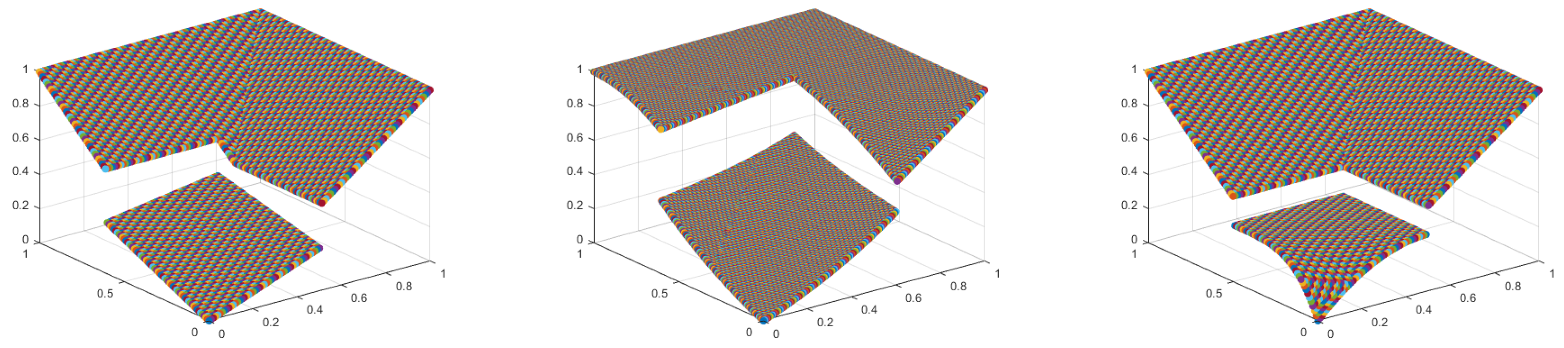
Example 1.

(1) For $\forall x,y\in [0,1],a,b\in (0,1),a\ne b$, the function $PQO:{[0,1]}^2\to [0,1]$ provided by

$$PQO(x,y)=\left\{\begin{array}{cc}xy\hfill & if0<x<a,0<y<b\hfill \\ min\{x,y\}\hfill & otherwise\hfill \end{array}\right.$$

is a pseudo-quasi overlap function

(2)

For $\forall x,y\in [0,1],k,l\ge 1,k\ne l,a\in (0,1)$, the function $PQO:{[0,1]}^2\to [0,1]$ provided by

$$PQO(x,y)=\left\{\begin{array}{cc}{x}^k{y}^l,\hfill & if0\le x\le a,0\le y\le a\hfill \\ \frac{2x^k{y}^l}{x+y}\hfill & otherwise\hfill \end{array}\right.$$

is a pseudo-quasi overlap functions.

(3)

For $\forall x,y\in [0,1]$, the function $PQO:{[0,1]}^2\to [0,1]$ provided by

$$PQO(x,y)=\left\{\begin{array}{cc}\frac{1+{(2x-1)}^2{(2y-1)}^4}{2},\hfill & if0.5\le x\le 1,0.5\le y\le 1\hfill \\ xy\hfill & otherwise\hfill \end{array}\right.$$

is a pseudo-quasi overlap function.

Certainly, we give the graphs of the above three pseudo-quasi overlap functions respectively, as shown in Figure 1.

Because properties of pseudo-quasi overlap functions are similar to properties of pseudo t-norms, they are not commutative and continuous. Thus, the following consider the relationship between pseudo-quasi overlap functions and pseudo-t-norms.

Definition 12.

A pseudo-t-norm is positive if $0<x\le 1,0<y\le 1$ such that $PT(x,y)>0$.

Definition 13.

An element is known as a nontrivial zero divisor of pseudo-t-norms when $x\in (0,1],y\in (0,1]$ fulfills $PT(x,y)=0$.

Theorem 1.

Let $PQO:{[0,1]}^2\to [0,1]$ be a bivariate function.

(1) 

If $PQO$ is an associative and continuous pseudo-quasi overlap function, then $PQO$ is a positive pseudo-t-norm.

(2) 

If $PQO$ is a positive pseudo t-norm, then $PQO$ is an associative pseudo-quasi overlap function.

(3) 

If $PQO$ is a pseudo-t-norm and it has no nontrivial zero divisor, then $PQO$ is an associative pseudo-quasi overlap function.

Proof. 

(1) Obviously, $PQO$ satisfied $(PT1),(PT2)$. Because $PQO$ is an associative and continuous pseudo-quasi overlap function, it follows that $PQO(0,1)=0,PQO(1,1)=1$. Then, for $\forall x\in [0,1]$, we can find y, and $0\le y\le 1,PQO(y,1)=x$. Consequently,

$$PQO(x,1)=PQO(PQO(y,1),1)=PQO(y,PQO(1,1))=PQO(y,1)=x.$$

Analogously, $PQO(1,x)=x$. Thus, $PQO$ satisfies $(PT3)$. Therefore, $PQO$ is a pseudo-t-norm. Indeed, $PQO$ is a positive pseudo-t-norm.

(2)

Directly, $PQO$ satisfied $(PQO2),(PQO3)$. Because $PQO$ is a pseudo-t-norm. Then

$$PQO(x,0)=PQO(0,x)=PQO(0,0)=0.$$

Moreover, $PQO$ is positive, so we know that $0<x\le 1,0<y\le 1$, and $PQO(x,y)>0$. Hence, if $PQO(x,y)=0$, then $x=0$ or $y=0$. Thus, $PQO$ satisfies $(PQO1)$. Therefore, $PQO$ is a pseudo-quasi overlap function. Moreover, $PQO$ satisfies associativity. Consequently, $PQO$ is an associative pseudo-quasi overlap function.

(3)

In fact, $PQO$ satisfies $(PQO2),(PQO3)$. Suppose that $PQO$ has no nontrivial zero divisor. In that way, if $0<x\le 1$, and $0<y\le 1$, so $PQO(x,y)\ne 0$. Hence, if $PQO(x,y)=0$, then $x=0$ or $y=0$. On the other hand, consider that $PQO$ is a pseudo-t-norm, we know that

$$PQO(x,0)=PQO(0,x)=PQO(0,0)=0.$$

Thus, $PQO$ satisfies $(PQO1)$. Therefore, $PQO$ is a pseudo-quasi overlap function. Indeed, $PQO$ is an associative pseudo-quasi overlap function. □

All quasi(pseudo)-overlap function are pseudo-quasi overlap functions. A continuous (commutative) pseudo-quasi overlap function is a quasi(pseudo)-overlap function. For the following theorem, we consider converting pseudo-quasi overlap functions into quasi(pseudo)-overlap functions.

Theorem 2.

Let ${QO}_1:{[0,1]}^2\to [0,1]$ and ${QO}_2:{[0,1]}^2\to [0,1]$ be two bivariate functions. If $PQO$ is a pseudo-quasi overlap function such that

$$\begin{array}{c}{QO}_1(x,y)=PQO(min\{x,y\},max\{x,y\})\\ {QO}_2(x,y)=PQO(max\{x,y\},min\{x,y\}).\end{array}$$

Then, ${QO}_1$ and ${QO}_2$ are two quasi-overlap functions.

Proof. 

If $PQO$ is a pseudo-quasi overlap function. Then,

$${QO}_1(x,y)=PQO(min\{x,y\},max\{x,y\})=PQO(min\{y,x\},max\{y,x\})={QO}_1(y,x).$$

Hence, $QO{}_1$ satisfies $(O1)$. If

$${QO}_1(x,y)=PQO(min\{x,y\},max\{x,y\})=0\mathrm{then}min\{x,y\}max\{x,y\}=0.$$

Hence, $x=0$ or $y=0$. Conversely, if $x=0$ or $y=0$, then, $PQO(min\{x,y\},$$max\{x,y\})=0$. Hence, ${QO}_1(x,y)=0$. Thus, $QO{}_1$ satisfies $(O2)$. Similarly, $QO{}_1$ satisfies $(O3)$. Take $\forall x,y,z\in [0,1],y\le z$, we know that $min\{x,y\}\le min\{x,z\}$, and $max\{x,y\}\le max\{x,z\}$. Moreover, according to $(O2)$, we know that

$${QO}_1(x,y)=PQO(min\{x,y\},max\{x,y\})\le PQO(min\{x,z\},max\{x,z\})={QO}_1(x,z).$$

Therefore, ${QO}_1$ satisfies $(O4)$. Indeed, ${QO}_1$ is a quasi-overlap function. Similarly, ${QO}_2$ is a quasi-overlap function. □

Definition 14.

An aggregation function is positive if $0<x\le 1,0<y\le 1$ fulfills $A(x,y)>0$.

Theorem 3.

Let $A:{[0,1]}^2\to [0,1]$ be an aggregation function, and $PQO$ is a pseudo-quasi overlap function such that

$$\begin{array}{c}PO(x,y)=A(PQO(x,y),PQO(y,x))\\ (QO(x,y)=A(PQO(x,y),PQO(y,x))).\end{array}$$

Then, $PO(QO)$ is a pseudo(quasi)-overlap function when and only when

(1) 

A is continuous (commutative);

(2) 

A is positive; and

(3) 

$A(x,y)=1\iff x=1$ and $y=1.$

Proof. 

(Necessity) Assume that $PO$ is a pseudo-overlap function, and

$$PO(x,y)=A(PQO(x,y),PQO(y,x)).$$

Items $(1)$ is direct. About $(2),(3)$. If $A(PQO(x,y),PQO(y,x))=0$, i.e.,

$$PQO(x,y)=PQO(y,x)=0.$$

Consequently, $x=0$ or $y=0$. Hence, if $x\in (0,1],y\in (0,1]$, then $A(x,y)>0$, that is, A is positive. Thus, A satisfies $(2)$. Similarly, A satisfies $(3)$.

(Sufficiency) Obviously, $PO$ satisfies $(O5)$. Suppose that A satisfies $(2)$ and

$$PO(x,y)=A(PQO(x,y),PQO(y,x)).$$

If $PO(x,y)=A(PQO(x,y),PQO(y,x))=0$ and A is positive, then $PQO(x,y)=0$ or $PQO(x,y)=0$. Consequently, $x=0$ or $y=0$. Conversely, $x=0$ or $y=0$, that is,

$$PQO(x,y)=PQO(y,x)=0.$$

Hence, $PO(x,y)=A(PQO(x,y),PQO(y,x))=A(0,0)=0$. Thus, $PO$ satisfies $(O2)$. Similarly, if A satisfies $(3)$, we know that $PO$ satisfies $(O3)$. Take $\forall x,y,z\in [0,1]$, $y\le z$. Then,

$$PO(x,y)=A(PQO(x,y),PQO(y,x))\le A(PQO(x,z),PQO(z,x))=PO(x,z).$$

Thus, $PO$ satisfies $(O4)$. Therefore, $PO$ is a pseudo-overlap function. Similarly, we get that $QO$ is a quasi-overlap function. □

Next, we present an expression form of pseudo quasi-overlap functions.

Lemma 2.

The function $PQO:{[0,1]}^2\to [0,1]$ is a pseudo-quasi overlap function if and only if

$$PQO(x,y)=\frac{f(x,y)}{f(x,y)+h(x,y).}$$

Take two binary functions $f,h$ defined on $[0,1]$, and fulfilling the following:

(1) 

$f$ is asymmetric or h is asymmetric;

(2) 

$f$ is non-decreasing and h is non-increasing;

(3) 

$f(x,y)=0\iff x=0$ or $y=0$;

(4) 

$h(x,y)=0\iff x=1$ and $y=1$; and

(5) 

$f$ is discontinuous or h is discontinuous.

Proof. 

The proof is analogous to [1]. □

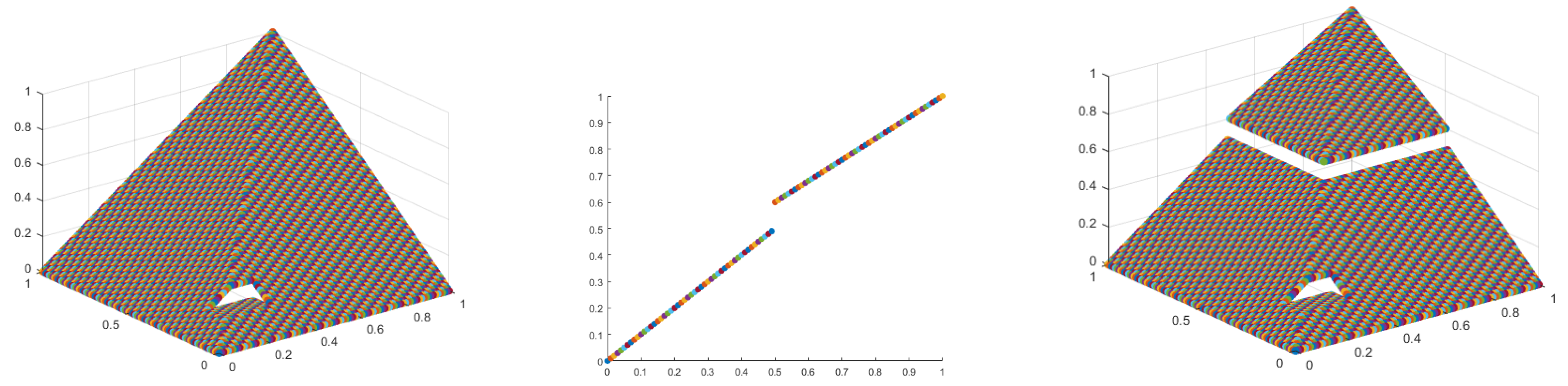
Example 2.

Take $a\in (0,1),f:{[0,1]}^2\to [0,1],h:{[0,1]}^2\to [0,1]$, separately, given by

$$f(x,y)={(xy)}^{\frac{1}{2}}$$

$$h(x,y)=\left\{\begin{array}{cc}max(-x+1,-y^2+1)\hfill & if0\le x\le a,0\le y\le a\hfill \\ max(-x+1,-y+1)\hfill & otherwise\hfill \end{array}\right..$$

Obviously, f is symmetric and continuous and g is asymmetric and discontinuous and satisfies the conditions of Lemma 2. Thus, $\forall x,y\in [0,1],a\in (0,1)$

$$PQO(x,y)=\left\{\begin{array}{cc}\frac{{(xy)}^{\frac{1}{2}}}{{(xy)}^{\frac{1}{2}}+max(-x+1,-y^2+1)}\hfill & if0\le x\le a,0\le y\le a\hfill \\ \frac{{(xy)}^{\frac{1}{2}}}{{(xy)}^{\frac{1}{2}}+max(-x+1,-y+1)}\hfill & otherwise\hfill \end{array}\right.$$

is a pseudo-quasi overlap function.

We give the graphs of the above $f,h,PQO=\frac{f}{f+h}$, respectively, as shown in Figure 2.

From Figure 2, we know the following.

(i) 

The image of f is continuous. The reason why the part indicated by the green arrow appears is that the differential value of the f at $x\to 0^{+}$ or $y\to 0^{+}$ is too large, i.e., $\underset{x\to 0^{+}}{lim}\frac{\partial f(x,y)}{\partial x}=\underset{y\to 0^{+}}{lim}\frac{\partial f(x,y)}{\partial y}=\infty$.

(ii) 

Similarly, the discontinuity in the image of $PQO=\frac{f}{f+h}$ is mainly reflected in the part indicated by the red arrow, excluding the part indicated by the green arrow. The reason why the part indicated by the green arrow appears is that the differential value of the $PQO=\frac{f}{f+h}$ at $x\to 0^{+}$ or $y\to 0^{+}$ is too large, i.e., $\underset{x\to 0^{+}}{lim}\frac{\partial PQO(x,y)}{\partial x}=\underset{y\to 0^{+}}{lim}\frac{\partial PQO(x,y)}{\partial y}=\infty$.

Corollary 1.

If the condition (1) of Lemma 2 is replaced by (1)’: f, h is symmetric. Then, $PQO$ is a quasi-overlap function.

Corollary 2.

If the condition (5) of Lemma 2 is replaced by (5)’: f, h is continuous. Then, $PQO$ is a pseudo-overlap function.

Corollary 3.

If the condition (1), (5) of Lemma 2 is replaced by (1)’: f, h is symmetric, (5)’: f, h is continuous. Then, PQO given by [1] is an overlap function.

Definition 15.

A binary function $PQG:{[0,1]}^2\to [0,1]$ is a pseudo-quasi group function if $\forall x,y\in [0,1]$, such that

$(PQG1)\mathcal{PQG}(x,y)=0\iff x=0$ and $y=0$;

$(PQG2)PQG(x,y)=1\iff x=1$ or $y=1$;

$(PQG3)PQG$ is nondecreasing.

Example 3.

(1) For $\forall x,y\in [0,1],a,b\in (0,1),a\ne b$, the function $PQG:{[0,1]}^2\to [0,1]$ provided by

$$PQG(x,y)=\left\{\begin{array}{cc}\frac{x+y-xy}{2}\hfill & ifx\in [0,a],y\in [0,b]\hfill \\ max(x,y)\hfill & otherwise\hfill \end{array}\right.$$

is a pseudo-quasi group function.

(2)

For $\forall x,y\in [0,1],a\in (0,1)$, the function $PQG:{[0,1]}^2\to [0,1]$ provided by

$$PQG(x,y)=\left\{\begin{array}{cc}\frac{x+y-2xy}{2-x-y}\hfill & ifx,y\in [0,a]\hfill \\ x+(1-x)(2y-y^2)\hfill & otherwise\hfill \end{array}\right.$$

is a pseudo-quasi group function.

(3)

For$\forall x,y\in [0,1],a,b\in (0,1)$, the function$PQG:{[0,1]}^2\to [0,1]$provided by

$$PQG(x,y)=\left\{\begin{array}{cc}\frac{1-{(1-2x)}^2{(1-2y)}^4}{3}\hfill & ifx\in [0,a],y\in [0,b]\hfill \\ max(x,y)\hfill & otherwise\hfill \end{array}\right.$$

is a pseudo-quasi group function.

We give the graphs of the above three pseudo-quasi group functions in Figure 3.

Indeed, the properties of pseudo-quasi group functions are similar to properties of pseudo t-conorms. They are not commutative and continuous. Consequently, the following consider the relationship between pseudo-quasi group functions and pseudo t-conorms.

Theorem 4.

Let $PQG:{[0,1]}^2\to [0,1]$ be a bivariate function.

(1) 

If $PQG$ is an associative and continuous pseudo-quasi group function, then $PQG$ is a positive pseudo t-conorm.

(2) 

If $PQG$ is a pseudo-t-conorm, and $xy<1,PQO(x,y)<1$, then $PQG$ is an associative pseudo-quasi overlap function.

Proof. 

(1) Obviously, $PQG$ satisfies $(PS1),(PS2)$. Because $PQG$ is an associative and continuous pseudo-quasi overlap function, it follows that $PQG(0,0)=0,PQG(1,0)=1$. Then, for $\forall x\in [0,1]$, we can find y fulfills $0\le y\le 1$, and $PQG(y,0)=x$. Consequently,

$$PQG(x,0)=PQG(PQG(y,0),0)=PQG(y,PQG(0,0))=PQG(y,0)=x.$$

Analogously, $PQG(0,y)=y$. Thus, $PQG$ satisfied $(PS3)$. Therefore, $PQG$ is a pseudo-t-conorm.

(2)

Directly, $PQG$ satisfies $(PQG1),(PQG3)$. Because $PQG$ is a pseudo-t-conorm, then

$$PQG(1,x)=PQG(x,1)=PQG(1,1)=1.$$

Moreover, if $xy<1$, then $PQO(x,y)<1$. Hence, if $PQG(x,y)=1$, then $x=1$ and $y=1$. Thus, $PQG$ satisfies $(PQG2)$. Therefore, $PQG$ is a pseudo-quasi group function. Besides, $PQG$ satisfies associativity. Consequently, $PQG$ is an associative pseudo-quasi group function. □

Obviously, all quasi(pseudo)-group functions are pseudo-quasi group functions. A continuous (commutative) pseudo-quasi group function is a quasi(pseudo)-group function. For the following theorem, we consider converting pseudo-quasi overlap groups into quasi(pseudo)-overlap groups.

Theorem 5.

Assume ${QG}_1:{[0,1]}^2\to [0,1]$ and ${QG}_2:{[0,1]}^2\to [0,1]$ to be two bivariate functions. If $PQG$ is a pseudo-quasi group function such that

$$\begin{array}{c}{QG}_1(x,y)=PQG(min\{x,y\},max\{x,y\})\\ {QG}_2(x,y)=PQG(max\{x,y\},min\{x,y\}),\end{array}$$

then, ${QG}_1$ and ${QG}_2$ are two quasi-overlap group functions.

Proof. 

The proof is analogous to Theorem 2. □

Theorem 6.

Let $A:{[0,1]}^2\to [0,1]$ be an aggregation function, and $PQG$ be a pseudo-quasi group function, such that

$$\begin{array}{c}PG(x,y)=A(PQG(x,y),PQG(y,x))\\ (QG(x,y)=A(PQG(x,y),PQG(y,x))).\end{array}$$

Then, $PG(QG)$ is a pseudo(quasi)-group function if and only if

(1) 

A is continuous (commutative);

(2) 

$A(x,y)=0\iff x=0$ and $y=0$; and

(3) 

$A(x,y)=1\Rightarrow x=1$ or $y=1$.

Proof. 

The proof is analogous to Theorem 3. □

Next, we present an expression form of pseudo-quasi group functions.

Lemma 3.

Let $f:{[0,1]}^2\to [0,1]$ and $h:{[0,1]}^2\to [0,1]$ be two unary functions, and $PQG:{[0,1]}^2\to [0,1]$ provided by

$$PQG(x,y)=-\frac{f(x,y)}{f(x,y)+h(x,y)}+1.$$

Then, $PQG$ is a pseudo-quasi group function if and only if it fulfills the following requirements:

(1) 

f is asymmetric or h is asymmetric;

(2) 

f is increasing and h is decreasing;

(3) 

$f(x,y)=0\iff x=1$ or $y=1$;

(4) 

$h(x,y)=0\iff x=0$ and $y=0$; and

(5) 

f is discontinuous or h is discontinuous.

Proof. 

The proof is analogous to Lemma 2. □

Example 4.

Take $a\in (0,1),f:{[0,1]}^2\to [0,1],h:{[0,1]}^2\to [0,1]$, respectively, given by

$$f(x,y)={(1-x-y+xy)}^{1/2}$$

$$h(x,y)=\left\{\begin{array}{cc}max(x,y^2)\hfill & if0\le x\le a,0\le y\le a\hfill \\ max(x,y)\hfill & otherwise\hfill \end{array}\right..$$

Obviously, f is symmetric and continuous, and h is asymmetric and discontinuous and satisfies the conditions of Lemma 3. Thus, $\forall x,y\in [0,1],a\in (0,1)$,

$$\mathcal{PQG}(x,y)=\left\{\begin{array}{cc}-\frac{{(1-x-y+xy)}^{1/2}}{{(1-x-y+xy)}^{1/2}+max(x,y^2)}+1\hfill & if0\le x\le a,0\le y\le a\hfill \\ -\frac{{(1-x-y+xy)}^{1/2}}{{(1-x-y+xy)}^{1/2}+max(x,y)}+1\hfill & otherwise\hfill \end{array}\right.$$

is a pseudo-quasi group function.

We give the graphs of the above $f,h,PQG=-\frac{f}{f+h}+1$, respectively, as shown in Figure 4.

From Figure 4, we know the following.

(i) 

The image of f is continuous. The reason why the part indicated by the green arrow appears is that the differential value of the f at $x\to 0^{+}$ or $y\to 0^{+}$ is too large, i.e., $\underset{x\to 0^{+}}{lim}\frac{\partial f(x,y)}{\partial x}=\underset{y\to 0^{+}}{lim}\frac{\partial f(x,y)}{\partial y}=\infty$.

(ii) 

Similarly, the discontinuity in the image of $PQG=-\frac{f}{f+h}+1$ is mainly reflected in the part indicated by the red arrow, excluding the part indicated by the green arrow. The reason why the part indicated by the green arrow appears is that the differential value of the $PQG=-\frac{f}{f+h}+1$ at $x\to 1^{-}$ or $y\to 1^{-}$ is too large, i.e., $\underset{x\to 1^{-}}{lim}\frac{\partial PQG(x,y)}{\partial x}=\underset{y\to 1^{-}}{lim}\frac{\partial PQG(x,y)}{\partial y}=\infty$.

Corollary 4.

If the condition $(1)$ of Lemma 3 is replaced by (1)’: f, h is symmetric. Then, $PQG$ is a quasi-overlap group.

Corollary 5.

If the condition $(5)$ of Lemma 3 is replaced by (5)’: f, h is continuous. Then, $PQG$ is a pseudo-overlap group.

Corollary 6.

If the condition $(1),(5)$ of Lemma 3 is replaced by (1)’: f, h is symmetric, (5)’: f, h is continuous. Then, $PQG$ is a group function.

Finally, we gain a means to structure pseudo-quasi overlap (group) functions by negative functions and pseudo-quasi group (overlap) functions.

Theorem 7.

Assume $N:[0,1]\to [0,1]$ to be a negation function and $PQO$ is a pseudo-quasi overlap function. Then, there exists a pseudo-quasi group function $PQG$ such that $\forall x,y\in [0,1]$,

$$PQG(x,y)=N(PQO(N(x),N(y))).$$

Proof. 

Suppose that N is a fuzzy negation, and $PQO$ is a pseudo-quasi overlap function. We need to prove that the function $PQG:{[0,1]}^2\to [0,1]$, defined by

$$PQG(x,y)=N(PQO(N(x),N(y))),$$

is a pseudo-quasi group function. If $x=y=0$, then $N(x)=N(y)=1$. Consequently,

$$PQO(N(x),N(y))=PQO(1,1)=1.$$

Thus, $PQG(0,0)=N(PQO(N(x),N(y)))=N(1)=0$. Contrarily, if

$$PQG(x,y)=N(PQO(N(x),N(y)))=0,$$

then $PQO(N(x),N(y))=1$. Consequently, $N(x)=N(y)=1$. Thus, $x=y=0$. Hence, $PQG$ satisfies $(PQG1)$. Similarly, $PQG$ satisfies $(PQG2)$. Consider $y,z\in [0,1]$ and $y\le z$. Then, $N(z)\le N(y)$. So, $PQO(N(x),N(z)))\le PQG(N(x),N(y)))$. Thus,

$$PQG(x,y)=N(PQO(N(x),N(y)))\le N(PQO(N(x),N(z)))=PQG(x,z).$$

Hence, $PQG$ satisfies $(PQG3)$. Therefore, $PQG$ is a pseudo-quasi group function. □

Theorem 8.

Let N: $[0,1]\to [0,1]$ be a negation function, and $PQG$ be a pseudo-quasi group function. Then, there exists a pseudo-quasi overlap function $PQO$, such that $\forall x,y\in [0,1]$,

$$PQO(x,y)=N(PQG(N(x),N(y))).$$

Proof. 

The proof is analogous to Theorem 7. □

Theorems 7 and 8 demonstrate the dual property of the pseudo-quasi overlap function and pseudo-quasi group function with regard to the negation function.

4. Additive Generators of Pseudo-Quasi Overlap Functions

In [38], an overlap function is constructed by two continuous and decreasing univariate functions. Thus, in this section, we give a method to structure pseudo-quasi overlap functions by two decreasing univariate functions $\theta ,\vartheta$, where $\theta$ satisfies discontinuity and $\vartheta$ satisfies discontinuity.

4.1. Additive Generators for Pseudo-Quasi Overlap Functions

First and foremost, we give the notion of additive generators based on pseudo-quasi overlap functions.

Definition 16.

Let $\theta :[0,1]\to [0,\infty ]$ and $\vartheta :[0,\infty ]\to [0,1]$ be two decreasing functions, where θ is discontinuous and ϑ is discontinuous. If a function $PQO : {[0,1]}^2\to [0,1]$ given by $PQO(x,y)=\vartheta (p\theta (x)+q\theta (y))$, for $\forall x,y\in [0,1],p\ne q,p,q\in (0,\infty )$, is a pseudo-quasi overlap function, then, a pair $(\vartheta ,\theta )$ is said to be an additive generator of pseudo-quasi overlap functions ${PQO}_{\vartheta ,\theta }$. More specifically, ${PQO}_{\vartheta ,\theta }$ is called a pseudo-quasi function additively generated by the pair $(\vartheta ,\theta )$.

Theorem 9.

Let $\theta :[0,1]\to [0,\infty ]$ and $\vartheta :[0,\infty ]\to [0,1]$ be two decreasing functions, and let θ be discontinuous or ϑ be discontinuous. For $\forall x,y\in [0,1],p\ne q,p,q\in (0,\infty )$, satisfying

(1) 

$x=0$ when and only when $\theta (x)=\infty$;

(2) 

$x=1$ when and only when $\theta (x)=0$;

(3) 

$x=0$ when and only when $\vartheta (x)=1$; and

(4) 

$x=\infty$ when and only when $\vartheta (x)=0$.

Then, $PQO : {[0,1]}^2\to [0,1]$ provided by

$$PQO(x,y)=\vartheta (p\theta (x)+q\theta (y))$$

is a pseudo-quasi overlap function.

Proof. 

Suppose that $\theta ,\vartheta$ are decreasing functions, and fulfill $(1),(2),(3),(4)$. If

$$PQO(x,y)=\vartheta (p\theta (x)+q\theta (y))=0,$$

then $p\theta (x)+q\theta (y)=\infty$. Consequently, $\theta (x)=\infty$ or $\theta (y)=\infty$. Thus, $x=0$ or $y=0$. Conversely, if $x=0$ or $y=0$, then $PQO(x,y)=\vartheta (p\theta (x)+q\theta (y))=0$. Thus, $PQO$ satisfies $(PQO1)$. In addition, if $PQO(x,y)=\vartheta (p\theta (x)+q\theta (y))=1$; that is, $p\theta (x)+q\theta (y)=0$, and then $\theta (x)=0$ and $\theta (y)=0$. Hence, $x=1$ and $y=1$. Thus, $PQO$ satisfies $(PQO2)$. Consider $\forall x,y,z\in [0,1],y\le z$, i.e., $\theta (y)\ge \theta (z)$. Then, $p\theta (x)+q\theta (y)\ge p\theta (x)+q\theta (z)$. Hence,

$$PQO(x,y)=\vartheta (p\theta (x)+q\theta (y))\le \vartheta (p\theta (x)+q\theta (z))=\mathcal{PQO}(x,z).$$

Thus, $PQO$ satisfies $(PQO3)$. Therefore, $PQO$ is a pseudo-quasi overlap function. □

Example 5.

Take $\theta :[0,1]\to [0,\infty ]$ and $\vartheta :[0,\infty ]\to [0,1]$, respectively, given by

$$\theta (x)=\left\{\begin{array}{cc}\infty \hfill & ifx=0\hfill \\ -2lnx\hfill & otherwise\hfill \end{array}\right.$$

$$\vartheta (x)=\left\{\begin{array}{cc}0\hfill & ifx=\infty \hfill \\ {(\frac{1}{e})}^x\hfill & if2<x<\infty \hfill \\ 1-\frac{x}{e}\hfill & otherwise\hfill \end{array}\right..$$

Obviously, $\theta (x)$ is continuous, $\vartheta (x)$ is discontinuous, and satisfies the conditions of Theorem 9. Then, for $\forall x,y\in [0,1],p\ne q,p,q\in (0,\infty )$,

$$PQO(x,y)=\vartheta (p\theta (x)+q\theta (y))=\left\{\begin{array}{cc}0\hfill & ifxy=0\hfill \\ x^{2p}{y}^{2q}\hfill & if0<x^p{y}^q<\frac{1}{e}\hfill \\ 1+\frac{1}{e}ln(x^{2p}{y}^{2q})\hfill & otherwise\hfill \end{array}\right.$$

is a pseudo-quasi overlap function.

We give the graphs of the above $\theta ,\vartheta ,PQO=\vartheta (p\theta +q\theta )$, in Figure 5.

Corollary 7.

If $p=q=1$ of Theorem 9, then, $PQO$ is a quasi-overlap function.

Corollary 8.

If $\theta ,\vartheta$ is continuous of Theorem 9, then, $PQO$ is a pseudo-overlap function.

Corollary 9.

If $p=q=1$, and $\theta ,\vartheta$ is continuous of Theorem 9. Then, $PQO$ given by [38] is an overlap function.

Table 1. Additive generators of overlap functions and pseudo-quasi overlap functions.

Function	Additive Generators of Overlap Functions	Additive Generators of Pseudo-Quasi Overlap Functions
formula	$O=\vartheta (p\theta +q\theta )$	$PQO=\vartheta (p\theta +q\theta )$
$p,q$	$p=q=1$	$p\ne q,p,q\in (0,\infty )$
$\theta ,\vartheta$	decreasing	decreasing
$\theta ,\vartheta$	continuous	$\theta$ is discontinuous or $\vartheta$ is discontinuous

shows that compared with the additive generators generated by overlap functions, the additive generators generated by pseudo-quasi overlap functions have fewer restriction conditions.

According to the above Theorem 9, we gain the following conclusions.

Corollary 10.

Let $\theta :[0,1]\to [0,\infty ]$ and $\vartheta :[0,\infty ]\to [0,1]$ be two decreasing functions, and θ is continuous, ϑ is discontinuous, and

(i) 

$x=1$ when and only when $\theta (x)=0$; and

(ii) 

$x=0$ when and only when $\theta (x)=\infty$.

If a function $\mathcal{PQO}:{[0,1]}^2\to [0,1]$ given by $\mathcal{PQO}(x,y)=\vartheta (p\theta (x)+q\theta (y))$ is a pseudo-quasi overlap function, then the conditions listed below are true:

 (1)

$x=\infty$ when and only when $\vartheta (x)=0$; and

 (2)

$x=0$ when and only when $\vartheta (x)=1$.

Proof. 

(1) Suppose that $\mathcal{PQO}(x,y)=\vartheta (p\theta (x)+q\theta (y))$ is a pseudo-quasi overlap function. (Sufficiency) Considering that $p\theta$ is continuous, and $p\theta (1)=0,p\theta (0)=\infty$. Then, for $\forall x\in [0,\infty ]$, we can find $x^{\prime },0\le x^{\prime }\le 1$, and satisfying $p\theta (x^{\prime })=x$. More importantly, according to $(i)$, we know that

$$\mathcal{PQO}(x^{\prime },1)=\vartheta (p\theta (x^{\prime })+q\theta (1))=\vartheta (p\theta (x^{\prime }))=\vartheta (x)=0.$$

Then, $x^{\prime }=0$. Thus, $x=p\theta (x^{\prime })=p\theta (0)=\infty$. (Necessity) If $x=\infty$, by item $(ii)$, so

$$\vartheta (x)=\vartheta (\infty )=\vartheta (\infty +\infty )=\vartheta (p\theta (0)+q\theta (0))=\mathcal{PQO}(0,0)=0.$$

Therefore, $\vartheta (x)=0⟺x=\infty$. $(2)$ Analogous to item $(1)$. □

Corollary 11.

Let $\theta :[0,1]\to [0,\infty ]$ and $\vartheta :[0,\infty ]\to [0,1]$ be two decreasing functions, and θ is discontinuous or ϑ is discontinuous, and

 (i)

$x=\infty$ when and only when $\vartheta (x)=0$; and

 (ii)

$x=0$ when and only when $\vartheta (x)=1$.

If the function $PQO$ given by $PQO(x,y)=\vartheta (p\theta (x)+q\theta (y))$ is a pseudo-quasi overlap function, then the conditions listed below are true:

 (1)

$x=1$ when and only when $\theta (x)=0$; and

 (2)

$x=0$ when and only when $\theta (x)=\infty$.

Proof. 

Suppose that $PQO(x,y)=\vartheta (p\theta (x)+q\theta (y))$ is a pseudo-quasi overlap function.

(1)

(Sufficiency) If $\theta (x)=0$. So, $PQO(x,x)=\vartheta (p\theta (x)+q\theta (x))=\vartheta (0)=1$. Thus, $x=1$. (Necessity) If $x=1$, then $PQO(x,x)=\vartheta (p\theta (x)+q\theta (x))=1$. Furthermore, according to $(ii)$, we know that, $p\theta (x)+q\theta (x)=0$. Thus, $\theta (x)=0$.

(2)

(Sufficiency) If $\theta (x)=\infty$, then $PQO(x,x)=\vartheta (p\theta (x)+q\theta (x))=\vartheta (\infty )=0$. Thus, $x=0$. (Necessity) If $x=0$. So, $PQO(x,1)=\vartheta (p\theta (x)+q\theta (1))=0$. Moreover, according to $(i),(1)$, we know that, $\infty =p\theta (x)+q\theta (1)=p\theta (x)+0=p\theta (x)$. Thus, $\theta (x)=\infty .$ □

Corollary 12.

Let ${PQO}_1 : {[0,1]}^2\to [0,1]$ and ${PQO}_2 : {[0,1]}^2\to [0,1]$ be two pseudo-quasi functions additively generated by the pair $({\vartheta }_1,{\theta }_1),({\vartheta }_2,{\theta }_2)$, separately. Consider the following states:

 (1)

If ${\theta }_1\le {\theta }_2$ and ${\vartheta }_2\le {\vartheta }_1$, then ${PQO}_2\le {PQO}_1$; and

 (2)

If ${\theta }_2\le {\theta }_1$ and ${\vartheta }_1\le {\vartheta }_2$, then ${PQO}_1\le {PQO}_2$.

Proof. 

We presume that ${PQO}_1(x,y)={\vartheta }_1(p{\theta }_1(x)+q{\theta }_1(y))$,

$${PQO}_2(x,y)={\vartheta }_2(p{\theta }_2(x)+q{\theta }_2(y)).$$

(1) If ${\theta }_1\le {\theta }_2$, then $p{\theta }_1(x)+q{\theta }_1(y)\le p{\theta }_2(x)+q{\theta }_2(y)$. Moreover ${\vartheta }_2\le {\vartheta }_1$, we know that,

$${\vartheta }_2(p{\theta }_2(x)+q{\theta }_2(y))\le {\vartheta }_1(p{\theta }_2(x)+q{\theta }_2(y))\le {\vartheta }_1(p{\theta }_1(x)+q{\theta }_1(y)).$$

Thus, ${PQO}_2\le {PQO}_1$. $(2)$ This is analogous to item $(1)$. □

4.2. Pseudo-Quasi Overlap Functions Generated by Pseudo-t-Norms and Pseudo Automorphisms

We recall the concept of pseudo automorphisms. Moreover, we introduce a method to construct pseudo-quasi overlap functions generated by pseudo-t-norms and pseudo automorphisms.

Definition 17

([38]). A unary function $H:[0,1]\to [0,1]$ is a pseudo automorphism if

 (1)

H is non-decreasing;

 (2)

H fulfills continuity;

 (3)

$x=1$ when and only when $H(x)=1$; and

 (4)

$x=0$ when and only when $H(x)=0$.

Lemma 4

([38]). A pseudo automorphism H is an automorphism if it is strictly increasing.

Theorem 10.

Let H be a pseudo automorphism, and $PT$ is a positive pseudo t-norm, and H is discontinuous or $PT$ is discontinuous. Then, a function ${PQO}_{H,PT}:{[0,1]}^2\to [0,1]$ provided by

$${PQO}_{H,PT}(x,y)=H(PT(x,y))$$

is a pseudo-quasi overlap function.

Proof. 

Suppose that H is a pseudo automorphism, $PT$ is positive, and H is discontinuous or $PT$ is discontinuous. So, $\forall x\in [0,1],PT(x,0)=PT(0,x)=PT(0,0)=0$. If $x=0$ or $y=0$, then ${PQO}_{H,T}(x,y)=H(PT(x,y))=H(0)=0$. Conversely, if

$${PQO}_{H,T}(x,y)=H(PT(x,y))=0,$$

then $PT(x,y)=0$. More importantly, $PT$ is positive. Hence, $x=0$ or $y=0$. Thus, ${PQO}_{H,T}$ satisfies $(PQO2)$. Similarly, ${PQO}_{H,T}$ satisfies $(PQO3)$. In addition, $PT$ and H are increasing functions, and then ${PQO}_{H,T}$ is also an increasing function. Thus, ${PQO}_{H,T}$ satisfied $(PQO1)$. Therefore, $PQO$ is a pseudo-quasi overlap function. □

Example 6.

(1) Take $0<c<e<d<1,0<a<1,PT : {[0,1]}^2\to [0,1],H:[0,1]\to [0,1]$, respectively, given by

$$PT(x,y)=\left\{\begin{array}{cc}c\hfill & ifc<x\le d,c<y\le e\hfill \\ min(x,y)\hfill & otherwise\hfill \end{array}\right.$$

$$H(x)=\left\{\begin{array}{cc}x\hfill & if0\le x<a\hfill \\ 0.8x+0.2\hfill & otherwise\hfill \end{array}\right..$$

Obviously, H is a pseudo automorphism, $PT$ is a positive and discontinuous pseudo-t-norm, and satisfies the conditions of Theorem 10. Then, $\forall x,y\in [0,1],0<a<1$,

$$PQO(x)=H(PT(x,y))=\left\{\begin{array}{cc}PT(x,y)\hfill & if0\le PT(x,y)<a\hfill \\ 0.8PT(x,y)+0.2\hfill & otherwise\hfill \end{array}\right.$$

is a pseudo-quasi overlap function.

We give the graphs of the above $PT,H,PQO=H(PT)$, individually, in Figure 6.

${PQO}_{H,PT}$ of Theorem 10 is said to be a pseudo-quasi overlap function generated by a pseudo-t-norm $PT$ and a pseudo automorphism H, or a pseudo-quasi overlap function generated by a $(H,PT)-$distortion.

Corollary 13.

If “H is discontinuous or $PT$ is discontinuous” of Theorem 10 is replaced by “$H,PT$ are continuous,” then, $PQO$ is a pseudo-overlap function.

Corollary 14.

If “$PT$ is a positive pseudo-t-norm” of Theorem 10 is replaced by “$PT$ is a positive t-norm,” then, $PQO$ is a quasi-overlap function.

Corollary 15.

If “H is discontinuous or $PT$ is discontinuous” and “$PT$ is a positive pseudo-t-norm” of Theorem 10 is replaced by “$H,PT$ are continuous” and “$PT$ is a positive t-norm”. Then, $PQO$ given by [38] is a overlap function.

Table 2. Overlap functions created by t-norms and pseudo isomorphisms and pseudo-quasi overlap functions created by pseudo-t-norms and pseudo isomorphisms.

Function	Overlap Functions Created by t-Norms and Pseudo Isomorphisms	Pseudo-Quasi Overlap Functions Created by Pseudo-t-Norms and Pseudo Isomorphisms
Formula	$O=H(T(x,y))$	$PQO=H(PT(x,y))$
$T/PT$	T is commutative	PT is noncommutative
H	non-decreasing	non-decreasing
$H,T/H,PT$	continuous	H is discontinuous or $PT$ is discontinuous

shows that pseudo-quasi overlap functions created by pseudo-t-norms and pseudo isomorphisms have fewer limitation conditions than overlap functions generated by t-norms and pseudo automorphisms.

Corollary 16.

Let $H:[0,1]\to [0,1]$ be an automorphism, $PT:{[0,1]}^2\to [0,1]$ is a pseudo-t-norm, and H is discontinuous or $PT$ is discontinuous. Then, a function ${PQO}_{H,T}$ given by ${PQO}_{H,PT}(x,y)=H(PT(x,y))$ is a pseudo-quasi overlap function if only and if $PT$ is positive.

Proof. 

(Necessity) If $PT(x,y)=0$, then ${PQO}_{H,T}(x,y)=H(PT(x,y))=H(0)=0$. Because ${PQO}_{H,T}$ is a pseudo-quasi overlap function, we are aware that $x=0$ or $y=0$. Thus, $PT$ is positive. (Sufficiency) This is analogous to Theorem 10. □

Corollary 17.

Let ${PQO}_{H,PT}$ be a pseudo-quasi overlap function generated by pseudo-t-norms $PT$ and pseudo automorphisms H. Then,

$$H(x)={PQO}_{H,PT}(x,1)={PQO}_{H,PT}(1,x)$$

Proof. 

${PQO}_{H,PT}(x,1)=$$H(PT(x,1))=H(x)=H(PT(1,x))$$={PQO}_{H,PT}(1,x)$. □

Corollary 17 provides a way to define a pseudo-automorphism H by a pseudo-quasi overlap function ${PQO}_{H,PT}$; that is, $H(x)={PQO}_{H,PT}(x,1)={PQO}_{H,PT}(1,x)$.

Corollary 18.

Let $PQO:{[0,1]}^2\to [0,1]$ be a pseudo-quasi overlap function. If $PQO$ is associative and continuous, then $PQO$ is a pseudo-quasi overlap function generated by a $(H,PQO)-$distortion.

Proof. 

If $PQO$ is associative and continuous, according to Theorem 1, we know that $PQO$ is a positive pseudo-t-norm. Consequently, $PQO(x,y)=H(PT(x,y))=H(PQO(x,y))$. Thus, $PQO$ is a pseudo-quasi overlap function generated by a $(H,PQO)-$distortion. □

Theorem 11.

Let $PQO:{[0,1]}^2\to [0,1]$ be a pseudo-quasi overlap function, and $H:[0,1]\to [0,1]$ be a pseudo automorphism. $PQO$ is generated by a $(H,PT)-$distortion ⇔$PT=H^{-1}·PQO,H(x)=PQO(x,1)=PQO(1,x)$.

Proof. 

(Necessity) Suppose that $PQO$ is a pseudo-quasi overlap function generated by a $(H,PT)-$distortion, i.e., $PQO=H·PT$. Then, $PT=H^{-1}·PQO$. Thus, by Corollary 17, $H(x)=PQO(x,1)=PQO(1,x)$. Indeed, $PT$ is a discontinuous pseudo-t-norm. (Sufficiency) Directly, $PT$ satisfies $(PT1)$. Because $H^{-1}$ and $PQO$ are increasing, it follows that $PT=H^{-1}·PQO$ is also increasing. Then, $PT$ satisfies $(PT2)$. Moreover,

$$PT(x,1)=H^{-1}(PQO(x,1))=H^{-1}(H(x))=x,$$

and $PT(1,x)=H^{-1}(PQO(1,x))=H^{-1}(H(x))=x$. Thus, T satisfies $(PT3)$. Therefore, $PT$ is a pseudo-t-norm. Moreover, if $PT(x,y)=H^{-1}(PQO(x,y))=0$. Then, $PQO(x,y)=0$. Thus, $x=0$ or $y=0$. Therefore, $PT$ is positive. Indeed, $PT$ is discontinuous. Finally, by Theorem 10, and $PQO=H·PT$, we know that $PQO$ is a pseudo-quasi overlap function generated by a $(H,PT)-$distortion. □

4.3. The Related Properties of Pseudo-Quasi Overlap Functions Generated by Additive Generators or $(H,PT)-$Distortions

We discuss the migrativity property of pseudo-quasi overlap functions generated by $(H,PT)-$distortions.

Theorem 12.

Let $H:[0,1]\to [0,1]$ be a pseudo automorphism, $PT:{[0,1]}^2\to [0,1]$ be a positive pseudo-t-norm, and H be discontinuous or $PT$ be discontinuous. Then, $PQO:{[0,1]}^2\to [0,1]$ is a pseudo-quasi overlap function generated by a $(H,PT)-$distortion if and only if $PQO$ is $PT$-migrative, and $H(x)=PQO(x,1)$.

Proof. 

(Necessity) Suppose that $PQO$ is a pseudo-quasi overlap function generated by additive generator and a $(H,PT)-$distortion, i.e., $PQO=H·PT$. Then,

$$\begin{array}{ll}PQO(PT(x,y),z)& =H(PT(PT(x,y),z)=H(PT(x,PT(y,z)))\\ & \hspace{1em}=PQO(x,PT(y,z)).\end{array}$$

Thus, $PQO$ is $PT$-migrative. Moreover, according to Corollary 17, we know that, $H(x)=PQO(x,1)$. (Sufficiency) If $PQO$ is $PT$-migrative, and $H(x)=PQO(x,1)$, then

$$PQO(x,y)=PQO(x,PT(y,1))=PQO(PT(x,y),1)=H(PT(x,y)).$$

Moreover, according to Theorem 10, we know that $PQO$ is a pseudo-quasi overlap function generated by a $(H,PT)-$distortion. □

We introduce the homogeneity property of pseudo-quasi overlap functions generated by $(\mathcal{H},\mathcal{PT})-$distortions.

Lemma 5

([38]). Let $H:[0,1]\to [0,1]$ be a pseudo automorphism, and $k\in [0,\infty ]$. H is homogeneous of order k $\iff H(x)=x^k$.

Lemma 6

([38]). Assume $H:[0,1]\to [0,1]$ to be a pseudo automorphism, and $k\in [0,\infty ]$. If H is homogeneous of order k, then $H^{-1}$ is also homogeneous of order $\frac{1}{k}$, and $H^{-1}=x^{\frac{1}{k}}$.

Theorem 13.

Assume $PQO$ to be a pseudo-quasi overlap function obtained by a $(H,PT)-$distortion, and $k_1\in [0,\infty ]$, H is a pseudo automorphism and homogeneous of order $k_1$. $PT$ is discontinuous and homogeneous of order $k_2$, where $k_2\in [0,\infty ]$ if and only if $PQO$ is homogeneous of order $k_1{k}_2$.

Proof. 

The proof is analogous to [38]. □

Theorem 14.

Let ${PQO}_{\vartheta ,\theta }$ be a pseudo-quasi overlap function additively generated by the pair $(\vartheta ,\theta )$. If ϑ and θ are homogeneous of order $k_1,k_2$, separately. Then, ${PQO}_{\vartheta ,\theta }$ is homogeneous of order $k_1{k}_2$.

Proof. 

Suppose that ${PQO}_{\vartheta ,\theta }$ is a pseudo-quasi overlap function additively created by the pair $(\vartheta ,\theta )$; that is, $PQO(x,y)=\vartheta (p\theta (x)+q\theta (y))$. Because $\vartheta$ and $\theta$ are homogeneous of order $k_1,k_2$, separately, then, $\vartheta (\alpha x)={\alpha }^{k_1}\vartheta (x)$, and $\theta (\alpha x)={\alpha }^{k_2}\theta (x)$. Consequently,

$$PQO(\alpha x,\alpha y)=\vartheta (p\theta (\alpha x)+q\theta (\alpha y))=\vartheta ({\alpha }^{k_2}(p\theta (x)+q\theta (y)))={\alpha }^{k_1{k}_2}\vartheta (p\theta (x)+q\theta (y)).$$

Thus, ${PQO}_{\vartheta ,\theta }$ is homogeneous of order $k_1{k}_2$. □

We study the idempotent property of a pseudo-quasi overlap function obtained by a $(H,PT)-$distortion.

Lemma 7

([38]). If $H:[0,1]\to [0,1]$ is an identity function, then, $H^{-1}$ is also an identity function, and $H^{-1}(x)=H(x)=x$.

Theorem 15.

Let $PQO$ be a pseudo-quasi overlap function acquired by a $(H,PT)-$distortion, and H be an identity function. If T is idempotent $\iff PQO$ is idempotent.

Proof. 

(Necessity) Suppose $PQO$ is a pseudo-quasi overlap function acquired by a $(H,PT)-$distortion; that is, $PQO(x,y)=H(PT(x,y))$. Then,

$$PQO(x,x)=H(PT(x,x))=H(x)=x.$$

Thus, $PQO$ is idempotent. (Sufficiency) According to Lemma 7, we know that

$$T(x,x)=H^{-1}(PQO(x,x))=H^{-1}(x)=x.$$

Thus, $PT$ is idempotent. □

5. Fuzzy Inference Triple I Methods Based on Pseudo-Quasi Overlap Functions

In this section, we give the definition of left-continuous pseudo-quasi overlap functions and the corresponding residual implication operator. In particular, we extend triple I algorithms to pseudo-quasi overlap functions, and study fuzzy inference triple I algorithms of residual implication operators provided by left-continuous pseudo-quasi overlap functions. Moreover, we give the solutions of expressions of the fuzzy inference triple I algorithms based on pseudo-quasi overlap functions for FMP and FMT problems.

Definition 18.

Let $PQO$ be a pseudo-quasi overlap function. $PQO$ is left-continuous when it fulfills $\forall x,y\in [0,1]$,

$PQO({\displaystyle \underset{i\in I}{\bigvee }}{x}_i,y)={\displaystyle \underset{i\in I}{\bigvee }}PQO(x_i,y)$ (left-continuous in the first variate)

$PQO(x,{\displaystyle \underset{j\in J}{\bigvee }}{y}_j)={\displaystyle \underset{j\in J}{\bigvee }}PQO(x,y_i)$ (left-continuous in the second variate).

As we know, a left-continuous pseudo-quasi overlap function can be continuous or discontinuous. If it is continuous, then it is a pseudo-overlap function. The left-continuous pseudo-quasi overlap function mentioned in this paper is discontinuous.

Definition 19.

Let $PQO$ be a left-continuous pseudo-quasi overlap function. Then, two residual implication operators $R_{PQO}^{(1)}:{[0,1]}^2\to [0,1]$, $R_{PQO}^{(2)}:{[0,1]}^2\to [0,1]$ defined by

$$R_{PQO}^{(1)}(x,y)=\bigvee \{z\in [0,1]\mid PQO(z,x)\le y\}$$

$$R_{PQO}^{(2)}(x,y)=\bigvee \{z\in [0,1]\mid PQO(x,z)\le y\}.$$

Theorem 16.

Let $PQO$ be a left-continuous pseudo-quasi overlap function. Then, the first residual implication operator $R_{PQO}^{(1)}$ and the second residual implication operator $R_{PQO}^{(2)}$ fulfill the conditions listed below:

 (i)

$PQO(z,x)\le y$ when and only when $z\le R_{PQO}^{(1)}(x,y)$, and also that $R_{PQO}^{(1)}$ is provided by

$$R_{PQO}^{(1)}(x,y)=\bigvee \{z\in [0,1]\mid PQO(z,x)\le y\}\mathit{;}$$

 (ii)

$PQO(x,z)\le y$ when and only when $z\le R_{PQO}^{(2)}(x,y)$, and also that $R_{PQO}^{(2)}$ is provided by

$$R_{PQO}^{(2)}(x,y)=\bigvee \{z\in [0,1]\mid PQO(x,z)\le y\}.$$

Proof. 

(i) (Necessity) Suppose that $R_{PQO}^{(1)}$ is provided by

$$C{R}_{PQO}^{(1)}(x,y)=\bigvee \{u\in [0,1]\mid PQO(z,x)\le y\}.$$

If $PQO(z,x)\le y$, So $z\le R_{PQO}^{(1)}(x,y)$. (Sufficiency) If $z\le R_{PQO}^{(1)}(x,y)$, then

$$z\le \bigvee \{u\in [0,1]\mid PQO(u,x)\le y\}.$$

In addition, $PQO$ is left-continuous in the first variate, we know that,

$$PQO(z,x)\le PQO(\bigvee \{z\in [0,1]\mid PQO(z,x)\le y\},x)$$

$$=\bigvee \{PQO(z,x)\mid PQO(z,x)\le y\}=y.$$

Consequently, $PQO(z,x)\le y$, and (ii) is analogous to (i). □

Corollary 19.

Let $PQO$ be a left-continuous pseudo-quasi overlap function, $R_{PQO}^{(1)}$ be the first residual implication operator and $R_{PQO}^{(2)}$ be the second residual implication operator of the $PQO$. The following conditions hold.

 (i)

$R_{PQO}^{(1)},R_{PQO}^{(2)}$ satisfies (NP) $\iff PQO$ has 1 as the neutral element;

 (ii)

$R_{PQO}^{(1)}(R_{PQO}^{(2)})$ satisfies (EP) $\iff PQO$ satisfies

$$PQO(PQO(x,y),z)=PQO(PQO(x,z),y)$$

$$(PQO(x,PQO(y,z))=PQO(y,PQO(x,z)))\mathit{;}$$

 (iii)

$R_{PQO}^{(1)}(R_{PQO}^{(2)})$ satisfies (IP) $\iff PQO$ fulfills $x\ge PQO(1,x)(x\ge PQO(x,1))$ whenever $x\in [0,1]$;

 (iv)

$R_{PQO}^{(1)}(R_{PQO}^{(2)})$ satisfies (LOP) $\iff PQO$ fulfills $x\ge PQO(1,x)(x\ge PQO(x,1))$ whenever $x\in [0,1]$;

 (v)

$R_{PQO}^{(1)}(R_{PQO}^{(2)})$ satisfies (ROP) $\iff PQO$ fulfills $x\le PQO(1,x)(x\le PQO(x,1))$ whenever $x\in [0,1]$;

 (vi)

$R_{PQO}^{(1)}(R_{PQO}^{(2)})$ satisfies (OP) $\iff PQO$ fulfills $x=PQO(1,x)(x=PQO(x,1))$ whenever $x\in [0,1]$;

 (vii)

$R_{PQO}^{(2)}$ satisfies (CB) $\iff PQO$ fulfills $x\bigwedge y\ge PQO(x,y)$ whenever $x,y\in [0,1]$;

 (viii)

$R_{PQO}^{(1)}(R_{PQO}^{(2)})$ satisfies (SIB) $\iff R_{PQO}^{(1)}(R_{PQO}^{(2)})$ satisfies (CB);

 (ix)

$R_{PQO}^{(1)},R_{PQO}^{(2)}$ satisfies (IB) $\iff x\bigwedge y=PQO(x,y)$;

 (x)

$R_{PQO}^{(1)},R_{PQO}^{(2)}$ satisfies (SBC), (LBC), and (RBC); and

 (xi)

$PQO$ has 1 as neutral element $\Rightarrow R_{PQO}^{(1)},R_{PQO}^{(2)}$ satisfies (CB).

Proof. 

The proof is direct. □

Example 7.

The following are three left-continuous pseudo-quasi overlap functions $PQO$ and its corresponding residual implication operators $R_{PQO}^{(1)},R_{PQO}^{(2)}$.

First, we give three important pseudo-quasi left-continuous overlap functions:

 (i)

$PQO(x,y)=\left\{\begin{array}{cc}xy\hfill & if0\le x\le a,0\le y\le a,and0<a<1,a\ne b\hfill \\ min\{x,y\}\hfill & otherwise\hfill \end{array}\right.$

 (ii)

$PQO(x,y)=\left\{\begin{array}{cc}x{y}^2\hfill & if0\le x\le a,0\le y\le a,and0<a<1\hfill \\ \frac{2xy}{x+y}\hfill & otherwise\hfill \end{array}\right.$

 (iii)

$PQO(x,y)=\left\{\begin{array}{cc}\frac{{(2x-1)}^2{(2y-1)}^4+1}{2}\hfill & if0.5<x\le 1,0.5<y\le 1\hfill \\ xy\hfill & otherwise\hfill \end{array}.\right.$

As we know, the image of the left-continuous pseudo-quasi overlap function in (i), (ii), and (iii) is similar to Figure 1.

Obviously, we know that

 (i)

$PQO(1,x)=min\{1,x\}=x$. Thus, $R_{PQO}^{(1)}$ satisfies (LOP), (ROP), i.e., $x\le y$ when and only when $R_{PQO}^{(1)}(x,y)=1$. Similarly, $R_{PQO}^{(2)}$ satisfies (LOP), (ROP), that is, $x\le y$ when and only when $R_{PQO}^{(2)}(x,y)=1$.

 (ii)

$PQO(1,x)=\frac{2x}{x+1}\ge x$. Thus, $R_{PQO}^{(1)}$ satisfies (ROP), that is, $R_{PQO}^{(1)}(x,y)=1\Rightarrow x\le y$. Similarly, $R_{PQO}^{(2)}$ satisfies (ROP), that is, $R_{PQO}^{(2)}(x,y)=1\Rightarrow x\le y$.

 (iii)

If $0\le x\le 0.5$, then $PQO(1,x)=x$. Thus, $R_{\mathcal{PQO}}^{(1)}$ satisfies (LOP), (ROP), i.e., $x\le y\iff R_{PQO}^{(1)}(x,y)=1$. If $0.5<x\le 1$, then $PQO(1,x)=\frac{1+{(2x-1)}^2}{2}$. Hence, $PQO(1,x)\le x$. Thus, $R_{PQO}^{(1)}$ satisfies (LOP), that is, $x\le y\Rightarrow R_{PQO}^{(1)}(x,y)=1$. Similarly, if $0\le x\le 0.5$, then $PQO(x,1)=x$. Thus, $R_{PQO}^{(2)}$ satisfies (LOP), (ROP); that is, $x\le y\iff R_{PQO}^{(2)}(x,y)=1$. If $0.5<x\le 1$, then $PQO(1,x)\le x$. Thus, $R_{PQO}^{(2)}$ satisfies(LOP), that is, $x\le y\Rightarrow R_{PQO}^{(2)}(x,y)=1$.

Thus, we obtain residual implication operators ${(i)}^{\prime },{(ii)}^{\prime },{(iii)}^{\prime }$ induced by the above left-continuous pseudo-quasi overlap functions $(i),(ii),and (iii)$. We have the following Figure 7, Figure 8 and Figure 9.

(i)’

$R_{PQO}^{(1)}=\left\{\begin{array}{cc}\frac{y}{x}\hfill & ify<x\le b\hfill \\ max\{a,y\}\hfill & ifx>y,andx>b\hfill \\ 1\hfill & otherwise\hfill \end{array}\right.$

$R_{PQO}^{(2)}=\left\{\begin{array}{cc}y\hfill & ify<x\le a\hfill \\ max\{\frac{y}{x},y\}\hfill & ifx>y,andx>a\hfill \\ 1\hfill & otherwise\hfill \end{array}\right.$

(ii)’

$R_{PQO}^{(1)}=\left\{\begin{array}{cc}\frac{y}{x^2}\hfill & ify<x\le a\hfill \\ \frac{xy}{2x-y}\hfill & ifx>y,andx>a\hfill \\ 1\hfill & otherwise\hfill \end{array}\right.$

$R_{PQO}^{(2)}=\left\{\begin{array}{cc}\sqrt{\frac{x}{y}}\hfill & ify<x\le a\hfill \\ \frac{xy}{2x-y}\hfill & ifx>y,andx>a\hfill \\ 1\hfill & otherwise\hfill \end{array}\right.$

(iii)’

$R_{PQO}^{(1)}=\left\{\begin{array}{cc}\frac{y}{x}\hfill & ify<x\le 0.5\hfill \\ \frac{\sqrt{2y-1}}{2{(2x-1)}^2}+\frac{1}{2}\hfill & ifx>y,andx>0.5\hfill \\ 1\hfill & otherwise\hfill \end{array}\right.$

$R_{PQO}^{(2)}=\left\{\begin{array}{cc}\frac{y}{x}\hfill & ify<x\le 0.5\hfill \\ \frac{\sqrt[4]{2y-1}\sqrt{2x-1}}{4x}+\frac{1}{2}\hfill & ifx>y,andx>0.5\hfill \\ 1\hfill & otherwise\hfill \end{array}\right.$

Definition 20.

Assume $R_{PQO}^{(1)}$ and $R_{PQO}^{(2)}$ be two operators with residual implications, $X,Y$ are nonempty universes, $F(x),F(y)$ are fuzzy sets on $X,Y$, separately, i.e., $A(x),A^{*}(x)\in F(x)$, $B(y)\in F(y)$, $0\le \alpha \le 1$,

$$\alpha \le R_{PQO}^{(1)}(R_{PQO}^{(1)}(A(x),B(y)),R_{PQO}^{(1)}(A^{*}(x),B^{*}(y)))$$

(1)

$$\alpha \le R_{PQO}^{(2)}(R_{PQO}^{(2)}(A(x),B(y)),R_{PQO}^{(2)}(A^{*}(x),B^{*}(y))).$$

(2)

If $B^{*}(y)$ is referred to as the tiniest fuzzy set on $F(y)$ by fulfill ing $(1)$ or $(2)$, then $B^{*}(y)$ is a solution of pseudo-quasi overlap function fuzzy inference α-triple I methods for FMP problem.

Theorem 17.

Let $R_{PQO}^{(1)}$ be an operator with residual implications produced by a left-continuous pseudo-quasi overlap function $PQO$ in the first variate. Then, a solution $B_{({\alpha }_1)}^{*}(y)$ of pseudo-quasi overlap function fuzzy inference α-triple I algorithms for $FM{P}_{({\alpha }_1)}$ problem is provided by

$$B_{({\alpha }_1)}^{*}(y)=\underset{x\in X}{\bigvee }\{PQO(PQO(\alpha ,R_{PQO}^{(1)}(A(x),B(y))),A^{*}(x))\}.$$

Proof. 

Obviously, $B_{({\alpha }_1)}^{*}(y)\ge PQO(PQO(\alpha ,R_{PQO}^{(1)}(A(x),B(y))),A^{*}(x))$. Assume that $R_{PQO}^{(1)}$ is an operator with residual implications produced by a left-continuous pseudo-quasi overlap function $PQO$ in the first variate. Then, according to Theorem 16 (i),

$$PQO(\alpha ,R_{PQO}^{(1)}(A(x),B(y)))\le R_{PQO}^{(1)}(A^{*}(x),B_{({\alpha }_1)}^{*}(y)).$$

Then,

$$\alpha \le R_{PQO}^{(1)}(R_{PQO}^{(1)}(A(x),B(y)),R_{PQO}^{(1)}(A^{*}(x),B^{*}(y))).$$

Additionally, assume that $C_{(1)}(y)$ is a fuzzy set on $F(y)$, and it satisfies $(1)$, i.e.,

$$\alpha \le R_{PQO}^{(1)}(R_{PQO}^{(1)}(A(x),B(y)),R_{PQO}^{(1)}(A^{*}(x),C_{(1)}(y))).$$

Because of Theorem 16 (i), we know that

$$R_{PQO}^{(1)}(A^{*}(x),C_{(1)}(y))\ge PQO(\alpha ,R_{PQO}^{(1)}(A(x),B(y)));$$

that is,

$$C_{(1)}(y)\ge PQO(PQO(\alpha ,R_{PQO}^{(1)}(A(x),B(y))),A^{*}(x)).$$

Thus, $B_{({\alpha }_1)}^{*}(y)\le C_{(1)}(y)$. Consequently, $B_{({\alpha }_1)}^{*}(y)$ is a solution of pseudo-quasi overlap function fuzzy inference $\alpha$-triple I methods for $FM{P}_{({\alpha }_1)}$ problem. □

Corollary 20.

If $\alpha =1$ of Definition 20, and $R_{PQO}^{(1)}$ satisfies (LOP). Then, a solution $B_{(1)}^{*}(y)$ of pseudo-quasi overlap function fuzzy inference α-triple I algorithms for $FM{P}_{(1)}$ problem is provided by

$$B_{(1)}^{*}(y)=\underset{x\in X}{\bigvee }\{PQO(PQO(R_{PQO}^{(1)}(A(x),B(y))),A^{*}(x))\}.$$

Theorem 18.

Let $R_{PQO}^{(2)}$ be an operator with residual implications produced by a left-continuous pseudo-quasi overlap function $PQO$ in the second variate. Then, a solution $B_{({\alpha }_2)}^{*}(y)$ of pseudo-quasi overlap function fuzzy inference α-triple I algorithms for $FM{P}_{({\alpha }_2)}$ problem is provided by

$$B_{({\alpha }_2)}^{*}(y)=\underset{x\in X}{\bigvee }\{PQO(A^{*}(x),PQO(R_{PQO}^{(2)}(A(x),B(y)),\alpha ))\},$$

Proof. 

Obviously, $B_{({\alpha }_2)}^{*}(y)\ge PQO(A^{*}(x),PQO(R_{PQO}^{(2)}(A(x),B(y)),\alpha ))$. We presume that $R_{PQO}^{(2)}$ is an operator with residual implications produced by a left-continuous pseudo-quasi overlap function $PQO$ in the second variate. Then, by Theorem 16 (ii), we know that

$$R_{PQO}^{(2)}(A^{*}(x),B_{(2)}^{*}(y))\ge PQO(R_{PQO}^{(2)}(A(x),B(y)),\alpha );$$

that is,

$$\alpha \le R_{PQO}^{(2)}(R_{PQO}^{(2)}(A(x),B(y)),R_{PQO}^{(2)}(A^{*}(x),B_{(2)}^{*}(y))).$$

Moreover, assume that $C_{(2)}(y)$ is a fuzzy set on $F(y)$, and it satisfies $(2)$; i.e.,

$$\alpha \le R_{PQO}^{(2)}(R_{PQO}^{(2)}(A(x),B(y)),R_{PQO}^{(2)}{A}^{*}(x),C_{(2)}(y))).$$

Because of Theorem 16 (ii), we know that

$$R_{PQO}^{(2)}(A^{*}(x),C_{(2)}(y))\ge PQO(R_{PQO}^{(2)}(A(x),B(y)),\alpha ).$$

Then,

$$PQO(A^{*}(x),PQO(R_{PQO}^{(2)}(A(x),B(y)),\alpha ))\le C_{(2)}(y).$$

Consequently, $C_{(2)}(y)\ge B_{({\alpha }_2)}^{*}(y)$. Thus, $B_{({\alpha }_2)}^{*}(y)$ is a solution of pseudo-quasi overlap function fuzzy inference $\alpha$-triple I methods for $FM{P}_{({\alpha }_2)}$ problem. □

Corollary 21.

If $\alpha =1$ of Definition 20, and $R_{PQO}^{(2)}$ satisfies (LOP). Then, a solution $B_{(2)}^{*}(y)$ of pseudo-quasi overlap function fuzzy inference α-triple I algorithms for $FM{P}_{(2)}$ problem is provided by

$$B_{(2)}^{*}(y)={\displaystyle \underset{x\in X}{\bigvee }}\{PQO(A^{*}(x),R_{PQO}^{(2)}(A(x),B(y)))\}.$$

Example 8.

Assume that $X=\{x_1,x_2,x_3\},Y=\{y_1,y_2,y_3\}$, take $\alpha =0.5,a=0.4,b=0.6$, and

$A=\{A(x_1),A(x_2),A(x_3)\}=\{0.3,0.5,0.7\}$

$B=\{B(y_1),B(y_2),B(y_3)\}=\{0.4,0.6,0.2\}$

$A^{*}=\{A^{*}(x_1),A^{*}(x_2),A^{*}(x_3)\}=\{0.8,0.4,0.1\}$

By Example 7 (i), (i)’, and Theorem 17, we know that

$$B_{({\alpha }_1)}^{*}(y_1)={\displaystyle \underset{x\in X}{\bigvee }}\{PQO(PQO(0.5,R_{PQO}^{(1)}(A(x),B(y_1))),A^{*}(x))\}=\bigvee \{0.5,0.4,0.04\}=0.5$$

$$B_{({\alpha }_1)}^{*}(y_2)={\displaystyle \underset{x\in X}{\bigvee }}\{PQO(PQO(0.5,R_{PQO}^{(1)}(A(x),B(y_2))),A^{*}(x))\}=\bigvee \{0.5,0.5,0.1\}=0.5$$

$$B_{({\alpha }_1)}^{*}(y_3)={\displaystyle \underset{x\in X}{\bigvee }}\{PQO(PQO(0.5,R_{PQO}^{(1)}(A(x),B(y_3))),A^{*}(x))\}=\bigvee \{0.5,0.16,0.1\}=0.5.$$

Thus, $B_{({\alpha }_1)}^{*}=\{B_{({\alpha }_1)}^{*}(y_1),B_{({\alpha }_1)}^{*}(y_2),B_{({\alpha }_1)}^{*}(y_3)\}=\{0.5,0.5,0.5\}$. Indeed, $\alpha =1$,

$$B_{(1)}^{*}=\{B_{(1)}^{*}(y_1),B_{(1)}^{*}(y_2),B_{(1)}^{*}(y_3)\}=\{0.8,0.8,\frac{2}{3})\}.$$

Similarly, $B_{({\alpha }_2)}^{*}=\{B_{({\alpha }_2)}^{*}(y_1),B_{({\alpha }_2)}^{*}(y_2),B_{({\alpha }_2)}^{*}(y_3)\}=\{0.5,0.5,0.1\}$. Furthermore, $\alpha =1,$

$$B_{(2)}^{*}=\{B_{(2)}^{*}(y_1),B_{(2)}^{*}(y_2),B_{(2)}^{*}(y_3)\}=\{0.8,0.8,0.2\}.$$

Definition 21.

Let $R_{PQO}^{(1)}$ and $R_{PQO}^{(2)}$ be two operators with residual implications, $X,Y$ are nonempty universes, $F(x),F(y)$ are fuzzy sets on $X,Y$, separately, i.e., $A(x)\in F(x),B(y),B^{*}(y)\in F(y),\alpha \in [0,1]$,

$$\alpha \le R_{PQO}^{(1)}(R_{PQO}^{(1)}(A(x),B(y)),R_{PQO}^{(1)}(A^{*}(x),B^{*}(y)))$$

(3)

$$\alpha \le R_{PQO}^{(2)}(R_{PQO}^{(2)}(A(x),B(y)),R_{PQO}^{(2)}(A^{*}(x),B^{*}(y))).$$

(4)

If $A^{*}(x)$ is called as the biggest fuzzy set on $F(x)$ by satisfying $(3)$ or $(4)$, then $A^{*}(x)$ is a solution of pseudo-quasi overlap function fuzzy inference α-triple I methods for the FMT problem.

Theorem 19.

Let $R_{PQO}^{(1)}$ and $R_{PQO}^{(2)}$ be two residual implication operators generated by a left-continuous pseudo-quasi overlap function $PQO$ in the first variate and in the second variate, respectively. Then, a solution $A_{({\alpha }_1)}^{*}(x)$ of a pseudo-quasi overlap function fuzzy inference α-triple I algorithm for $FM{T}_{({\alpha }_1)}$ problem is provided by

$$A_{({\alpha }_1)}^{*}(x)={\displaystyle \underset{y\in Y}{\bigwedge }}\{R_{PQO}^{(2)}(PQO(\alpha ,R_{PQO}^{(1)}(A(x),B(y))),B^{*}(y))\}.$$

Proof. 

Obviously, $R_{PQO}^{(2)}(PQO(\alpha ,R_{PQO}^{(1)}(A(x),B(y))),B^{*}(y))\ge A_{({\alpha }_1)}^{*}(x)$. Suppose that $R_{PQO}^{(1)}$ and $R_{PQO}^{(2)}$ are operators with residual implications produced by a left-continuous pseudo-quasi overlap function $PQO$ in the first variate and in the second variate, respectively. Then, by Theorem 16, we know that

$$B^{*}(y)\ge PQO(PQO(\alpha ,R_{PQO}^{(1)}(A(x),B(y)),A_{({\alpha }_1)}^{*}(x));$$

that is,

$$R_{PQO}^{(1)}(A_{({\alpha }_1)}^{*}(x),B^{*}(y))\ge PQO(\alpha ,R_{PQO}^{(1)}(A(x),B(y))).$$

Consequently,

$$R_{PQO}^{(1)}(R_{PQO}^{(1)}(A(x),B(y)),R_{PQO}^{(1)}(A_{({\alpha }_1)}^{*}(x),B^{*}(y)))\ge \alpha .$$

In addition, suppose that $D_1(x)$ is a fuzzy set on $F(x)$, it also fulfills $(3)$, i.e.,

$$R_{PQO}^{(1)}(R_{PQO}^{(1)}(A(x),B(y)),R_{PQO}^{(1)}(D_{(1)}(x),B^{*}(y)))\ge \alpha .$$

By Theorem 16, we know that

$$R_{PQO}^{(1)}(D_{(1)}(x),B^{*}(y))\ge PQO(\alpha ,R_{PQO}^{(1)}(A(x),B(y))).$$

Then,

$$B^{*}(y)\ge PQO(PQO(\alpha ,R_{PQO}^{(1)}(A(x),B(y)),D_{(1)}(x)).$$

Consequently,

$$D_{(1)}(x)\le R_{PQO}^{(2)}(PQO(\alpha ,R_{PQO}^{(1)}(A(x),B(y))),B^{*}(y)).$$

Hence, $A_{({\alpha }_1)}^{*}(x)\ge D_{(1)}(x)$. Thus, $A_{({\alpha }_1)}^{*}(x)$ is a solution of pseudo-quasi overlap function fuzzy inference $\alpha$-triple I methods for $FM{T}_{({\alpha }_1)}$ problem. □

Corollary 22.

If $\alpha =1$ in Definition 21, and $R_{PQO}^{(1)}$ satisfies (LOP). Then, a solution $A_{(1)}^{*}(y)$ of a pseudo-quasi overlap function fuzzy inference α-triple I algorithm for $FM{T}_{(1)}$ problem is provided by

$$A_{(1)}^{*}(x)={\displaystyle \underset{y\in Y}{\bigwedge }}\{R_{PQO}^{(2)}(R_{PQO}^{(1)}(A(x),B(y)),B^{*}(y))\}.$$

Theorem 20.

Let $R_{PQO}^{(1)}$ and $R_{PQO}^{(2)}$ be two operators with residual implications produced by a left-continuous pseudo-quasi overlap function $PQO$ in the first variate and in the second variate, respectively. Then, a solution $A_{({\alpha }_2)}^{*}(y)$ of pseudo-quasi overlap function fuzzy inference α-triple methods for $FM{T}_{({\alpha }_2)}$ problem is provided by

$$A_{({\alpha }_2)}^{*}(x)={\displaystyle \underset{y\in Y}{\bigwedge }}\{R_{PQO}^{(1)}(PQO(R_{PQO}^{(2)}(A(x),B(y)),\alpha ),B^{*}(y))\}.$$

Proof. 

Obviously, $A_{({\alpha }_2)}^{*}(x)\le R_{PQO}^{(1)}(PQO(R_{PQO}^{(2)}(A(x),B(y)),\alpha ),B^{*}(y))$. Consider that $R_{PQO}^{(1)}$ and $R_{PQO}^{(2)}$ are operators with residual implications produced by a left-continuous pseudo-quasi overlap function $PQO$ in the first variate and in the second variate respectively. Then, by Theorem 16, we know that

$$B^{*}(y)\ge PQO(A_{({\alpha }_2)}^{*}(x),PQO(R_{PQO}^{(2)}(A(x),B(y)),\alpha ));$$

that is,

$$PQO(R_{PQO}^{(2)}(A(x),B(y)),\alpha )\le R_{PQO}^{(2)}(A_{({\alpha }_2)}^{*}(x),B^{*}(y)).$$

Hence,

$$R_{PQO}^{(2)}(R_{PQO}^{(2)}(A(x),B(y)),R_{PQO}^{(2)}(A_{({\alpha }_2)}^{*}(x),B^{*}(y)))\ge \alpha .$$

In addition, assume that $D_2(x)$ is a fuzzy set on X, and it satisfies $(4)$, i.e.,

$$\alpha \le R_{PQO}^{(2)}(R_{PQO}^{(2)}(A(x),B(y)),R_{PQO}^{(2)}(D_{(2)}(x),B^{*}(y))).$$

According to Theorem 16, we know that,

$$PQO(R_{PQO}^{(2)}(A(x),B(y)),\alpha )\le R_{PQO}^{(2)}(D_{(2)}(x),B^{*}(y));$$

that is,

$$B^{*}(y)\ge PQO(D_{(2)}(x),PQO(R_{PQO}^{(2)}.(A(x),B(y)),\alpha ))$$

Then,

$$D_{(2)}(x)\le R_{PQO}^{(1)}(PQO(R_{PQO}^{(2)}(A(x),B(y)),\alpha ),B^{*}(y)).$$

Thus, $A_{({\alpha }_1)}^{*}(x)\ge D_{(2)}(x)$. Therefore, $A_{({\alpha }_2)}^{*}(x)$ is a solution of pseudo-quasi overlap function fuzzy inference $\alpha$-triple I methods for $FM{T}_{({\alpha }_2)}$ problem. □

Corollary 23.

If $\alpha =1$ in Definition 21, and $R_{PQO}^{(2)}$ satisfies (LOP), then a solution $A_{(2)}^{*}(y)$ of a pseudo-quasi overlap function fuzzy inference triple I method for $FM{T}_{(2)}$ problem is given by

$$A_{(2)}^{*}(x)={\displaystyle \underset{y\in Y}{\bigwedge }}\{R_{PQO}^{(1)}(R_{PQO}^{(2)}(A(x),B(y)),B^{*}(y))\}.$$

Example 9.

Suppose that $X=\{x_1,x_2,x_3\},Y=\{y_1,y_2,y_3\}$, taking $\alpha =0.6,a=0.5,b=0.3$,

$A=\{A(x_1),A(x_2),A(x_3)\}=\{0.4,0.7,0.5\}$

$B=\{B(y_1),B(y_2),B(y_3)\}=\{0.1,0.8,0.6\}$

$B^{*}=\{B^{*}(y_1),B^{*}(y_2),B^{*}(y_3)\}=\{0.9,0.5,0.2\}$.

By Example 7 (i), (i)’, and Theorem 19, we know that,

$A_{({\alpha }_1)}^{*}(x_1)={\displaystyle \underset{y\in Y}{\bigwedge }}\{R_{PQO}^{(2)}(PQO(0.6,R_{PQO}^{(1)}(A(x_1),B(y))),B^{*}(y))\}=\bigwedge \{1,\frac{5}{6},\frac{1}{3}\}=\frac{1}{3}$

$A_{({\alpha }_1)}^{*}(x_2)={\displaystyle \underset{y\in Y}{\bigwedge }}\{R_{PQO}^{(2)}(PQO(0.6,R_{PQO}^{(1)}(A(x_2),B(y))),B^{*}(y))\}=\bigwedge \{1,\frac{5}{6},0.5\}=0.5$

$A_{({\alpha }_1)}^{*}(x_2)={\displaystyle \underset{y\in Y}{\bigwedge }}\{R_{PQO}^{(2)}(PQO(0.6,R_{PQO}^{(1)}(A(x_2),B(y))),B^{*}(y))\}=\bigwedge \{1,\frac{5}{6},\frac{1}{3}\}=\frac{1}{3}$.

Thus, $A_{({\alpha }_1)}^{*}=\{A_{({\alpha }_1)}^{*}(x_1),A_{({\alpha }_1)}^{*}(x_2),A_{({\alpha }_1)}^{*}(x_3)\}=\{\frac{1}{3},0.5,\frac{1}{3}\}$. Indeed, $\alpha =1,$

$A_{(1)}^{*}=\{A_{(1)}^{*}(x_1),A_{(1)}^{*}(x_2),A_{(1)}^{*}(x_3)\}=\{0.2,\frac{1}{3},0.2\}$.

Similarly, $A_{({\alpha }_2)}^{*}=\{A_{({\alpha }_2)}^{*}(x_1),A_{({\alpha }_2)}^{*}(x_2),A_{({\alpha }_2)}^{*}(x_3)\}=\{0.5,0.5,0.5\}$. Furthermore, $\alpha =1,$

$A_{(2)}^{*}=\{A_{(2)}^{*}(x_1),A_{(2)}^{*}(x_2),A_{(2)}^{*}(x_3)\}=\{0.5,0.5,0.5\}$.

6. Conclusions

In this paper, we delete the commutativity and continuity of overlap functions, and propose the definition of pseudo-quasi overlap functions and relative property. Furthermore, we present a structure method of pseudo-quasi overlap functions. Then, based on the above pseudo-quasi overlap functions, we discuss additive generators of pseudo-quasi overlap functions. Additionally, we construct an expression of pseudo-quasi overlap functions through pseudo-t-norms and pseudo automorphisms. Finally, we combine pseudo-quasi overlap functions with triple I algorithms, and investigate fuzzy inference triple I methods of residual implication operators provided by left-continuous pseudo-quasi overlap functions.

The research findings in this paper have some guiding significance for the selection of various generalized overlap functions. Furthermore, it provides theoretical foundations for the practical application of overlap functions. Zhang [39] studied partial triangular norms and their corresponding residual implication operators, which are very meaningful topics. In future research work, we will study the partial triangular norm and implication operators on intuitionistic fuzzy sets. On the other hand, the research results in [40,41] have good application prospects, which not only lays a theoretical foundation for Takagi–-Sugeno (T-S) fuzzy system with successive time-delay (STD), but also provide new ideas for our future research direction. In the next research process, we discuss the application of pseudo-quasi overlap function fuzzy inference methods in T-S fuzzy system.