
Axiomatics of the Observer Manifold and Relativity


Laboratoire de Mathématiques de Reims (CNRS, UMR9008), Université de Reims Champagne-Ardenne, Moulin de la Housse, B.P. 1039, CEDEX 2, F-51687 Reims, France
Axioms 2023, 12(2), 205; https://doi.org/10.3390/axioms12020205
Submission received: 1 January 2023
/
Revised: 9 February 2023
/
Accepted: 11 February 2023
/
Published: 15 February 2023
(This article belongs to the Section Hilbert’s Sixth Problem)
Abstract
:We show that Special and General Relativity lead to the introduction of an observer manifold, in addition to the usual event manifold. Axiomatics that require that manifolds be Hausdorff are not appropriate for the observer manifold. We propose an alternative axiomatics and show how most of the usual local computations extend to this framework without difficulty. The derivation of the Lorentz transformation takes a new meaning in this context, enabling the identification of the representations of several observers and hence reducing the observer manifold to the event manifold. However, we show in an example relevant to the radiation of accelerated electrons that this identification is not always correct. This appears to be relevant in any situation where gravitational fields in remote locations have to be measured on Earth, such as the detection of gravitational waves, or when high accelerations are involved, such as in electron radiation or laser cooling.
Keywords:
axiomatics of manifolds; Lorentz transformation; conformal metric; special relativity; general relativity; observer manifold; event manifoldPACS:
04.20.Cv; 04.80.CcMSC:
83C99; 53B301. Introduction
The axiomatics of manifold theory is still in flux because not all authors agree on whether manifolds should share all the local or global properties of Euclidean space, such as the Hausdorff separation axiom, or whether one should postulate the existence or a covering by an increasing sequence of compact sets. Such subtleties are well-known to be necessary in some mathematical questions [1], (p. 11, [2]), including some model space-times (pp. 173–174, [3]), [4]; however, they did not arise in the problems that were tackled during the early history of manifold theory [5]. We discuss another setting here, relevant for all models of space-time, that requires yet another modification of the axiomatics of manifold theory, eschewing all axioms of a global nature: the mathematization of the notion of observer manifold in General Relativity. Élie Cartan had suggested that “local” observers should have “infinitesimal” features that have no mathematical counterpart in the definition of what we now call the event manifold [6]. However, he did not pursue these ideas towards a modification of the axiomatics of manifolds, although he reiterated, in his lectures on Riemannian manifolds, that the notion of manifold is still “difficult” to define (p. 57, [7]). The later discussion of the forms of the Equivalence Principle [8] that we shall recall at greater length below showed that the distinction of the event and observer manifolds was necessary for the physical interpretation of General Relativity, leading to the C-equivalence principle [9,10]. Any situation in which gravitational fields at different points are being compared, such as the Pound–Rebka experiment, cannot be interpreted without C-equivalence. The postulate that General Relativity reduces to Special Relativity at the linear approximation must therefore be relaxed because, otherwise, there would be no way to infer a difference in gravitational fields by a redshift measurement. Mathematically, this leads to relaxing the Strong Equivalence principle into the C-equivalence principle, while keeping the Weak Equivalence principle [9,10].
Our goal here is to revisit these developments from a purely mathematical point of view, showing that a proper axiomatic formulation still allows for most of the usual calculations of a local nature to go through unchanged. The essential new element is the integration into the mathematical formalism of physical aspects of C-equivalence [9,10], leading to a modification of the axiomatics of manifolds. As an application, we determine the evolution of the conformal factor relating two observers in a simple model of a beam of accelerated electrons that could be a prototype for related situations involving strong accelerations and/or strong gravitational fields.
We restrict attention to smooth differential manifolds, although some obvious generalizations to topological, PL manifolds (“piecewise-linear”, such as polyhedra) or analytic manifolds could be formulated; however, such extensions do not seem relevant to General Relativity at the present time.
We first recall in Section 2 the evolution of the physical postulates of General Relativity, focusing on the strong and weak equivalence principles, and show how the C-equivalence principle gives a mathematically consistent expression of these physical postulates. We then give two axiomatic definitions for the event and observer manifold, respectively (Section 3). Section 4 shows that the usual axiomatics of manifold theory is only relevant for the event manifold. In particular, the Hausdorff axiom, which requires, intuitively, that small enough neighborhoods of two distinct points will not intersect if they are taken small enough, should be given up because the local space-times of observers attached to different particles that happen to meet at one point are not necessarily locally reducible to the same Minkowski space by the choice of an orthonormal tetrad. Nonetheless, the new definition is sufficient for introducing tensor calculus and, therefore, for performing most usual calculations of a local nature. As an example, we show that the derivation of the fact that the Lorentz transformation does not require reciprocity between observers [11] may be transferred verbatim to this setting, just as the characterization of conformal transformations in the context of C-equivalence [12,13]. An application to electron radiation is outlined in Section 5.
The two main points of this paper are that the observer manifold is not the event manifold, and that the observer manifold need not be Hausdorff. They may be explained in intuitive terms as follows.
The axiomatics of Special Relativity, recalled in Section 2, make two postulates. First, it is assumed that there are inertial observers attached to material systems in uniform translation away from gravitational or other fields. These observers are supposed to have access to a standard apparatus that includes standard rods and clocks, and to be able to communicate with each other through the exchange of light signals that travel at the speed c, a speed that does not depend on the observer. By assumption, they are able to assign to any event a set of four coordinates that do not necessarily have any direct meaning, but that do provide unique labels. Second, one also assumes that it is possible to transform the coordinates of each observer into the coordinates of a Minkowski space, in which coordinates now have a metrical meaning, and the metric takes the form . Another inertial observer may do the same, but in the framework of Special Relativity, its transformed coordinates, say (, 1, 2, 3), may be transformed into the of the first observer by a Lorentz transformation, possibly after a change of origin. The physical consequences derived from this notion of “inertial observer” are numerous and very well supported by experiment. However, interpretation requires one to assign to an elementary particle with nonzero rest mass, such as a meson, a local inertial observer that travels with it. That is how we account for the fact that the lifetime of a meson in its inertial system differs from its lifetime in the lab system. Now, no human observer exists that would so to say “ride along an elementary particle”, and could perform the operations allowed by the postulates of Special Relativity. The observers of the theory are therefore notional observers, rather than actual observers: the operations of coordinate assignment and coordinate change are never actually carried out, except possibly for the “laboratory system”. When several observers in relative uniform motion meet at a spacetime point, their notional observers are related by Lorentz transformation, so that there is for them only one Minkowski space in which all their translational motions take place, but this identification of notional observers has no reason to hold for non-uniform motions. It is possible to circumvent this difficulty by postulating instead that the de Broglie wave of a particle includes, through its dynamics, the elements of a local system attached to it [14]. This wave is a purely material object that is represented in the theory by the notional observer associated with the particle. The observers in the sequel are always understood in this sense; they do not require human intervention and, indeed, such intervention is generally not feasible.
Since there is no reason to identify all observers to one another, one must distinguish two manifolds: the event manifold on the one hand, of which the points may be viewed as the set of events labeled by coordinates by a given observer, say the “laboratory system", and the observer manifold on the other hand that consists of all the notional observers attached in principle to every portion of the trajectory of any system that may be assimilated to a particle.
Thus, the “points” of an observer manifold are actually themselves Hausdorff manifolds in the usual sense: to every spacetime point A of the trajectory of a particle, we associate an observer representing the system in which it would be at rest; for this observer, events in some neighborhood of A form a small part of a Lorentzian Manifold that contains the point A. It may not be possible to assign a well-defined observer to any object of large extension since the notion of rigid body does not make sense in Special or General Relativity, and it may not be defined by a single de Broglie wave, with the significant exception of the de Broglie wave of a Bose–Einstein condensate.
In general, if A is one of the points on the trajectory of a given particle, there is no reason to assume that the manifold is independent of the state of motion of the particle, or the gravitational field around it—in fact, C-equivalence shows that it must depend on the local gravitational field through a conformal factor, and the discussion of Section 2 shows that, given the current experimental evidence, there is no other freedom. If all events A corresponding to the successive positions of the particle under consideration happen to be recorded by another observer, such as the “laboratory observer” with origin O, we obtain the event manifold if we replace all the manifolds with the manifold .
From the point of view of the “laboratory system”, the event manifold is the set of events as recorded in this laboratory, but each of these events is viewed by other observers in terms of different manifolds. Therefore, the observer manifold is not a set of points, but a set of local space-times of different observers, and these space-times are themselves manifolds in the usual sense. Different observers compare their descriptions using transfer maps that should not be confused with maps representing coordinate changes between coordinate patches of the same manifold. The local space-times of observers are not locally reducible to Minkowski space-time, but are conformally Minkowskian, reflecting the action of the local gravitational field on the measurement apparatus—it is this feature that amounts to giving up the Strong Equivalence Principle that explains the name of “C-equivalence”. Even when the space-time paths of observers cross in the event manifold, their local space-times will be different.
This intuitive view of the observer manifold immediately implies that the Hausdorff axiom in the usual form cannot be correct. If two spacetime trajectories meet at some event, called A for the first trajectory, and B for the second, we must have , but not necessarily . Since the two particles involved represent all events in a neighborhood of , any neighborhood of the A-particle must contain the event B for the B-particle, see Figure 1. Therefore, it is impossible to find non-intersecting neighborhoods of these two trajectories, even though their local observers are different whenever .
When several particles meet at one point at the same time, these notional observers are therefore not necessarily the same. Only in the case of particles in relative translational motion with constant velocity can we assert that the representations of the events by the two observers are related by a Lorentz transformation, so that they may both be viewed as evolving in the same Minkowski space, as we show next.
2. C-Equivalence as a Mathematical Expression of Einstein’s Equivalence Principle
C-equivalence builds on attempts to give a mathematical form to Einstein’s physical views about the equivalence principle. The evolution of ideas involved three steps: First, Einstein’s modification of Special Relativity to take into account non-inertial systems led him to introduce what we now call the Strong Equivalence Principle. Second, closer analysis, mostly by Dicke and his coworkers, showed that it was necessary to introduce a second postulate, the Weak Equivalence Principle. Third, the fact, well-supported by experiments, that all material objects, including the measurement apparatus, are affected by gravitational fields led to the replacement of the Strong Equivalence Principle by the C-equivalence Principle. We examine these steps in order.
2.1. Einstein’s Physical Picture
Let us revisit the early arguments that go back to Einstein’s analysis of the devolution of his own reasoning [15], in the light of later developments.
Special Relativity is based on measurements performed in inertial systems. Dynamics cannot be developed within Special Relativity from the point of view of an observer S exterior to a system that is subject to applied forces. At the same time, the comoving system attached to , however one defines it, cannot be considered as an inertial system, neither globally—since the velocity S relative to varies at every instant and every point of the trajectory of —nor locally—since the measuring apparatus of is subject to the same forces. As a consequence, the laws of Special Relativity are of no avail to . Nonetheless, a generalization of Special Relativity is necessary since all material objects, including instruments used for measurement, are always subject to a gravitational field—say, of the Earth—and this field is universal—it affects all material particles, not just those possessing a certain “charge” or “color”, etc. Therefore, Special Relativity may only enjoy partial, local validity.
This inability to keep the notion of an inertial system in the presence of a universal field suggests giving up the equivalence of observers at rest relative to each other—that is, the very basis of the notion of an inertial system. The goal of the theory is then to coordinate the observations carried out by different observers, taking into account the influence of physical fields on the observed phenomena and on the measuring devices. A theory that realizes this program ipso facto yields a theory of space and time as well as a theory of “universal” fields of forces and, in particular, of the gravitational field. Einstein put forth such a theory by suggesting that one should extend the Principle or Relativity to accelerated motions, hence the name of General Relativity that this theory has received. Let us now see how this extension leads to a first form of the equivalence principle, and how later facts showed the need for a scrutiny of its postulational basis, both physically and mathematically.
2.2. Early Arguments Leading to the First Form of the Equivalence Principle
Recall that there are three notions of mass: inertial mass, passive gravitational mass, and active gravitational mass. When we write Newton’s law for a particle A falling freely in the Earth’s gravitational field, we write the familiar equation
Here, the mass m of A occurs on both sides of this equation: on the left, it is an inertial mass; on the right, a (passive) gravitational mass subject to the attraction of the mass M of the Earth. By contrast, the mass M plays in this equation the role of an active gravitational mass. In addition, m would be interpreted as an active gravitational mass if we considered the motion of the Earth under the (tiny) gravitational field of the particle. Let us assume that all three masses are the same. In that case, m cancels out of the equations of motion and, furthermore, in a domain in which the gradient of the gravitational field is negligible, all bodies fall with the same acceleration, irrespective of their nature. It follows that the action of gravity on test particles should admit of a purely geometrical representation, based, as Einstein showed, on a Lorentzian manifold.
If we disregard the difference between events, the coordinates that label them, and the observers that assign these coordinates, one may be tempted to say that achieving a representation of the relation between gravity and Special Relativity is to perform a local (nonlinear) change of coordinates such that, with respect to the new system, equations of motion have the same form as in Special Relativity. This amounts to eliminating the local force field by choosing as a local inertial system the inertial system instantaneously dragged by a material point subject to this field. Then, if one disregards the behavior of the measurement devices, one may postulate that the laws of Physics should be generalized so as to satisfy the following postulate:
Strong equivalence principle. In a domain in which the gradient of the universal force field is negligible, one may always perform a change of local coordinate chart that ensures that Special Relativity remains locally valid.
However, if we take this form of strong equivalence too literally, it is at variance with another desirable requirement, namely general covariance:
Principle of general covariance. Laws of Physics should be covariant by general changes of coordinates.
This contradiction, or more precisely, the fact that the current mathematical expression of Einstein’s equivalence principle was not satisfactory, was perceived very early [13,16,17], (p. 69, [18]), [19]. Indeed, general covariance is unable to provide a specific principle for any physical theory, since coordinates need not have any direct physical meaning—only scalars and geometric objects do. Einstein immediately concurred but kept appealing to it as an intuitive basis of his theory.
His position may be understood if one distinguishes two interpretations of the principle. First, general covariance expresses the demand that the laws of Physics should not depend on the way events are labeled by sets of coordinates; it can form the basis of no specific theory. Second, this mathematical covariance is coupled with a physical covariance: the independence of our theoretical formulation from the system of reference in which it is formulated. Here, a system of reference S differs from another one not by the choice of coordinates, but by the fact that, relative to a third one , they are in a different state of motion. In this sense, for Einstein, this physical covariance achieves an extension of the principle of Special Relativity, the latter being only valid for inertial systems in uniform translation. Einstein therefore restricted the class of possible systems of reference to those that may locally be reduced to systems of inertia, allowing the local change of system of reference to be nothing but a change of coordinates, so that physical covariance was not distinguished from mathematical covariance. Analysis of this issue led to a scrutiny of the finer structure of Einstein’s equivalence principle [20,21,22,23]. It became clear that Einstein’s equivalence principle was the combination of three principles listed below, of which the content is made precise in the next four subsections:
- (a)
- The weak equivalence principle;
- (b)
- The identity of local descriptions of phenomena, independently of the region of homogeneous field under consideration;
- (c)
- The identification of this local description with the one performed by Special Relativity, that is, one postulates:
- (c1)
- Local isotropy;
- (c2)
- The existence of measuring devices having the same behavior as in a system of inertia.
Let us examine these points in order.
2.3. Weak Equivalence
Weak equivalence essentially follows from the local identity of inertial mass and passive gravitational mass—an identity vouched for at a precision of by the experiments by Eötvös, revisited by Dicke et al. It postulates nothing as regards active gravitational mass, since the principle of action and reaction is only valid in Newtonian Mechanics. A precise formulation is the following:
Weak equivalence assumes that trajectories of test bodies in free fall are independent of the mass or composition of these bodies. We may view them as distinguished curves of the space-time of an observer that records this free fall.
All authors seem to take these curves to be geodesics of the space-time of this observer.
2.4. Identity of Local Descriptions
The issue is this: to what extent are ratios of physical magnitudes “of the same kind” independent of the situation of the observer in the field of forces? This assumes one can define such magnitudes of the same kind at different places. One may, with R.H. Dicke [24,25,26,27,28], consider that the ratio of the masses of two bodies may be considered to be independent of their localization with respect to the force field. Indeed, otherwise, when moving from one point to the other, one of the bodies would undergo a modification of its internal energy, in a proportion different from what the other would undergo, and this variation of energy should correspond to the work of an additional force if both bodies are to describe a geodesic of the local spacetime. Such anomalous forces are not observed. Naturally, this does not by itself warrant the equality of the ratio of masses: in fact, one could, following R. H. Dicke, imagine that these anomalous forces are compensated by an additional field. The upshot of his analysis is that this field cannot be a tensor field if one also postulates the isotropy of the local spacetime. It cannot be a vector field for this that leads to a contradiction with weak equivalence. It cannot be a scalar field either if one also postulates that the constants of Physics do not vary from point to point. We consider in the sequel that none of these fields exist and the local descriptions of phenomena “of the same kind” are identical.
2.5. Isotropy of Local Spacetime
The assumption that spacetime should be locally isotropic is supported by the experiments by Beltran-Lopez, Hughes and Robinson [29,30]. These experiments, the idea of which goes back to Cocconi and Salpeter, conclude that the anisotropy of the energy distribution in our galaxy has no influence on the inertial mass by showing:
- (1)
- That the Zeeman effect of and is independent of the orientation of the external magnetic field with respect to the center of our galaxy, despite the fact that, according to semi-classical theory, an electron of nonzero orbital momentum has, in the various magnetic states, velocities of different directions with respect to ;
- (2)
- That the distribution of the magnetic states of the Lithium nucleus is not modified by effects of mass anisotropy.
We shall therefore assume that the local space-time is isotropic. This allows for inhomogeneities in matter distribution so that space-time is neither homogeneous nor globally isotropic, except possibly in (large-scale) cosmological models that do not concern us here.
2.6. Standard Measurement Devices and C-Equivalence
To postulate strong equivalence, that is, the inertial character of any local system of reference, is to admit the existence at least theoretically of measurement devices that have Minkowskian behavior everywhere even though one considers at the same time the influence of the gravitational field on all physical objects, including measurement devices. C-equivalence modifies the equivalence principle to avoid this contradiction. The physical postulates of C-equivalence, to which we give a mathematical formulation in the other sections of this paper, are therefore the following:
All local observers are provided with standard measuring devices (identical devices having the same behavior at the same point when relatively at rest); however, because of the presence of the field, these devices have a behavior that varies from point to point. This may be expressed, taking into account the assumptions we made in the previous three sections, bywhere the elementary squared interval between two events is according to an observer located at A, but would be according to an inertial observer. The quantity is not accessible to experiments, since cannot be measured when a nonzero field is present, but the ratio comparing the deviations from Special Relativity at two different points A and B is accessible to measurement.
According to this perspective, local spacetime is conformal to a neighborhood of Minkowski spacetime (hence the name “C-equivalence”), and the local system of reference will be called a pseudo-inertial system.
We shall say that a theory is compatible with C-equivalence if it is consistent with
- Weak equivalence;
- The identity of local descriptions of identical phenomena;
- Isotropy of local spacetime;
- The pseudo-inertial character of the local system of reference.
Remark 1.
It is apparent that in (2) does not determine any additional scalar field because it is not a function on the event manifold.
Remark 2.
Since C-equivalence requires a change of coordinates (to transform locally g to η) and a gauge change (to replace by 1) for the local system to be inertial, it allows for distinguishing between mathematical covariance and physical covariance. However, this transformation does not take place on the event manifold, but on a manifold that plays the role of a “point” in the observer manifold, so that there is no contradiction with general covariance.
We now proceed to a mathematical framework that gives expression to these physical principles. In a nutshell, since the local systems of different observers cannot be identified as tangent spaces of a single event manifold because their metric cannot be reduced to the Minkowski metric, it is necessary to introduce one manifold for each observer in each state of motion. This leads to an observer manifold that is not a manifold in the usual sense. Its “points” are themselves manifolds in the usual sense. The comparison of the measurement of different observers is achieved via transfer maps that are not coordinate changes.
3. Axiomatics of the Event and Observer Manifolds
Let us consider the axiomatic frameworks that give mathematical expression to the postulates of the previous section. We begin with the notion of manifold in the usual sense. Most authors would agree that “manifolds are spaces that locally look like n-space”. The usual definition (p. 2, [31]) may be spelled out as follows, recalling standard terminology in the process.
Definition 1.
A (differential) manifold M of dimension n and of class , where or , is a set equipped with a family , called an atlas, indexed by an arbitrary set Z such that
- (Cov)
- (Covering axiom.) For every , the set is a subset of M. Furthermore, any point of M belongs to at least one .
- (CA)
- (Coordinate axiom.) Each is an open subset of , the latter being endowed with its usual topology, and the are one-to-one. Therefore, each point P of may be written for some α, where is uniquely determined by α. These n numbers are called the local coordinates of P in the coordinate chart .
- (CC)
- (Axiom on coordinate changes.) If two coordinate charts and are such that , the map is of class on its domain of definition, and so is its inverse .
One defines a topology on M by saying that a set is open if, for any coordinate chart , the sets are open in . Submanifolds are defined in the obvious way.
By construction, each map is a homeomorphism between and . We shall deal throughout with smooth manifolds () for simplicity. The definitions of geometric objects, including tensors and connections, are standard [3,32], including more general “geometric objects” such as Lie derivatives (p. 18 sq., [33]). In particular, a Lorentzian manifold is a manifold endowed with a metric tensor with signature (with three negative squares).
Even though satisfies the Hausdorff separation axiom, M may not. An example (see e.g., (Figure 5, p. 14, [3])) is given by , where , and . One may endow it with an atlas , where and . Let the map send to x if , and to x if . Similarly, let , if , and if . For the topology on M induced by this atlas, any open set in M that contains necessarily contains because any neighborhood of 0 in the real line contains both positive and negative points. However, . M does not satisfy the Hausdorff axiom.
For such reasons, some authors require further topological conditions of a local or global nature (p. 1, [34]), [32] that all imply the Hausdorff separation axiom. Some of them are so strong that any manifold in this sense may be embedded in a space of sufficiently high dimension [35], (p. 12, [34]). Still, Élie Cartan was not satisfied with these developments (p. 57, [7]); he thought another formalism would be better suited to General Relativity and stressed the need for an observer manifold without formalizing it. Bourbaki, also aware of the difficulty of the subject, remained non-committal, and merely published a list of results on manifolds [36]; the only non-conventional feature in this booklet is to allow local charts in which the may be open sets in a space that could depend on the chart (§ 5.1.1., p. 34, [36]).
We focus on four dimensions for simplicity, since we shall need no other. Similarly, we only consider Lorentz metrics even though the extension to Riemannian metrics is straightforward. We now define the notions of event manifold and observer manifold.
Definition 2.
An event manifold is a (smooth, differential) manifold M of dimension 4 and of class . An observer manifold , over the event manifold M, is a family , indexed by an arbitrary set , such that
- 1.
- Each is a Lorentzian manifold (typically consisting of only one chart) with a distinguished origin .
- 2.
- Each has a trace on M that contains . This trace represents the trajectory of on the event manifold M.
- 3.
- If two I and J are such that , then there are open sets and , in and , respectively, related by a diffeomorphism .
- 4.
- .
Each of the will be called the system of reference of the observer at , or observer for short. These are not necessarily associated with a human observer in any sense, but to a splitting of space and time provided by a local de Broglie wave [14]. The map connects the representations of events in systems and ; it will be called a transfer map. It should not be confused with coordinate changes on a manifold.
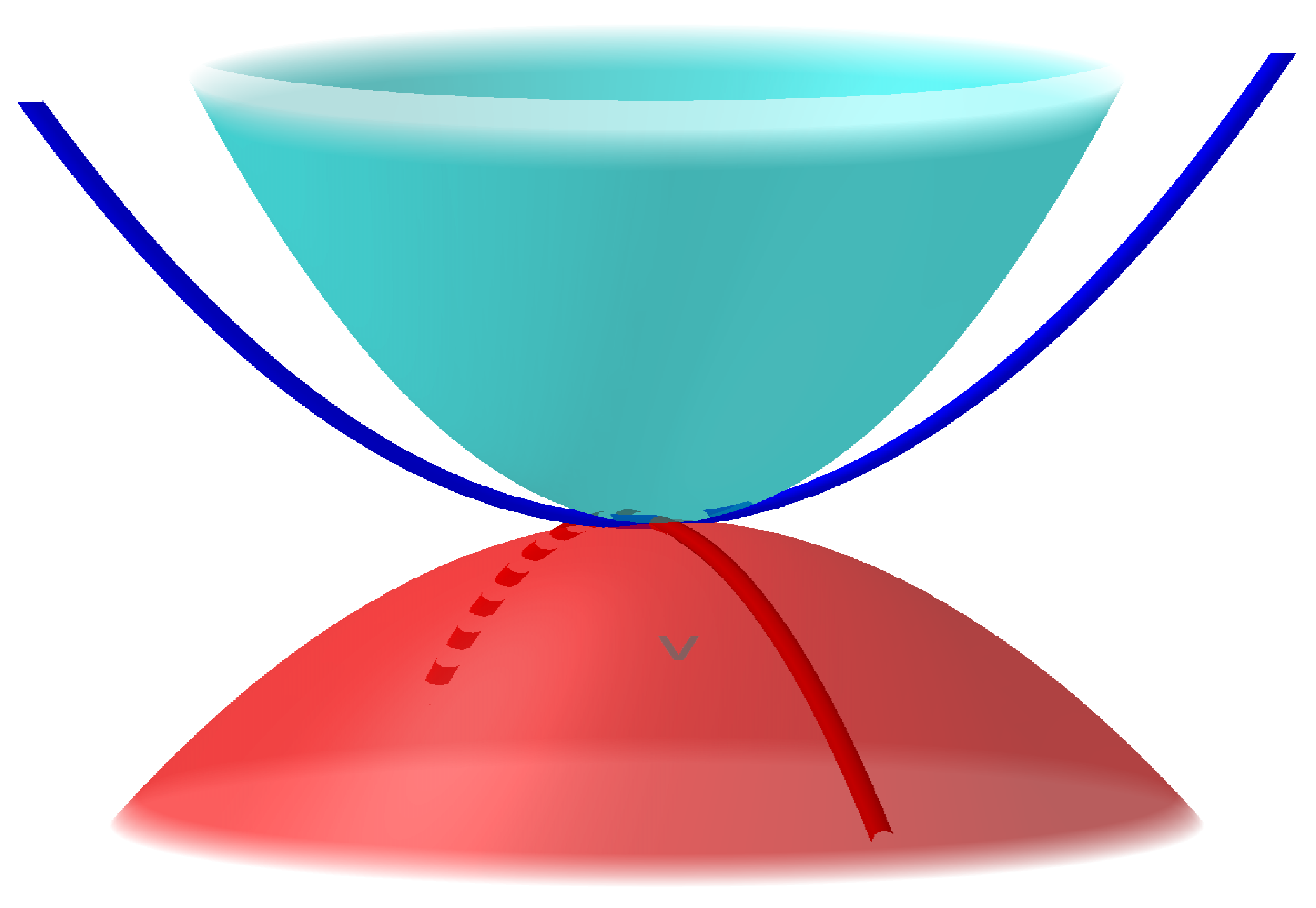
Thus, the observer manifold is not, in general, a manifold, but a collection of manifolds that may not have any simple global structure. An intuitive picture may be given by Figure 1 in which two systems and are represented as surfaces (in red and blue, respectively). Their traces and on M are indicated by lines of the same colors, but M itself is not represented to avoid clutter. In this example, and coincide, but they belong to different systems so that it is not possible to find a neighborhood of that would exclude . It is therefore impossible to reduce the observer manifold to the event manifold without removing all the information about the observers other than their instantaneous position. Therefore, the event manifold does not contain, in general, all the physical or mathematical information in the observer manifold. As we shall see next, there is an exception: various observers may all be related to one another to form a global Minkowski space if we are within Special Relativity.
4. The Postulational Basis of Special Relativity
Let us briefly relate the mathematical postulates from a physical viewpoint. The primitive notion in any physical theory is that of a reference system. For example, system S consists of an observer located at the origin O of this system and that can determine, using standard clocks and rods:
- a.
- The time interval separating two given events;
- b.
- The interval of length separating these two events.
Standard rods and clocks are those that have the same behavior when they stand at the same point and are at rest relatively to one another. Their existence is an unprovable postulate of Special Relativity. In this section, we identify such systems with the systems of an observer manifold in the sense of the previous section; we shall define a mathematical notion of inertial observer and show the following result.
Theorem 1.
Let be an observer manifold in which the following hold:
- (In)
- All observers are inertial, meaning that, for every I, the manifold is a Minkowski space with coordinates , and any point that moves in uniform rectilinear motion in also has the same property with respect to any in which the same motion may be represented (that is, for those such that ).
- (UTr)
- Any two observers S and are in uniform translation with respect to one another. Mathematically, this means that, if are the coordinates of the origin of in system S, then its 3-velocity measured in S is constant. A similar property holds for .
- (VL)
- With respect to any inertial system, light propagates in vacuo isotropically and with the same speed c.
Then, the transfer maps, in the sense of Definition 2, between any two observers S and are Lorentz transformations. In addition, the velocity of S with respect to is equal in length to that of with respect to S: reciprocity between inertial systems is a mathematical consequence of the postulates.
Remark 3.
Galilean kinematics also postulates an equivalence of inertial systems for the determination of space and time, but it is not compatible with postulate (VL) of the constancy of the velocity of light.
Remark 4.
Proof.
Let us consider two inertial systems S and on , with local coordinates and ( or any Greek index , Latin indices run from 1 to 3); we are interested in the correspondence between the representations of any event in both systems. All considerations are local, in a small neighborhood of the origins of S and , and all functions involved are assumed to be smooth. This transfer map has the form
since it depends on the spatial velocity of the origin of as measured in S. The conventions of tensor calculus, including the summation convention, all apply. Let . The matrix is therefore the Jacobian matrix of the map . Since is a diffeomorphism,
Axioms (In) and (UTr) then ensure [13,37,38] that there is a covariant vector such that may be written
Here, the are functions of . The proof of this result is recalled at the end of this section.
Assumption (VL) ensures that space-time intervals and corresponding to the same elementary light path are proportional. In other words, there is a scalar such that
Since both metrics must have the same signature, is positive. Since both observers are inertial by (In), we may also assume
Therefore, we have
Differentiating (8) with respect to , and taking (5) into account, we obtain
Now, by (8), terms such as or may be simplified. After performing these simplifications, we are left with
This holds for all values of the indices. Let us fix an arbitrary value for index : , and choose , where . For these index values, we have, since is diagonal, and . Equation (9) therefore yields . However, since was arbitrary, we obtain for all values of . A similar argument, letting in (9), shows that , for all values of . In addition, substituting into (5) yields . To summarize, we have proved that (again for all values of the indices),
The are therefore affine functions of the :
and, conversely, we may write:
where
We now proceed to show that
First, note that a change of the direction of the space axes of S leaves the factor unchanged, so that, with a convenient abuse of notation,
On the other hand, since the two inertial systems S and play symmetric roles, we also have
where is the velocity of S with respect to . Since, by (6), we also have , it follows that
Equations (8) and (17) then yield
whence
and, in particular,
Now, Equation (13) expresses that any fixed point in has coordinates in S that are affine functions of . It follows that the 3-velocity of S with respect to is equal to . We therefore have an expression for (and, similarly, for the 3-velocity of w.r.t. S):
Let us now relate the 3-velocities of S w.r.t. and w.r.t. S. Letting in (19) and in (), and using (23), we obtain
Indeed, setting in (19), we obtain
Equation (25) is obtained similarly.
Equation (24) now yields, after taking (22) into account, . Using now (25), we obtain . Simplifying this using (18), we obtain , hence
and, consequently,
QED.
We have therefore proved that the passage from the to the is a Lorentz transformation, and that , which is what we set out to prove. □
We conclude this section by recalling the gist of the proof of Equation (5). It is a consequence of axiom (UTr) that expresses that uniform motions are the same in both systems. A direct proof is as follows [37]. Consider a point M in uniform motion with respect to both S and . Its trajectory may be written , where , are constants. Similarly, it may be represented in in the form . The corresponding 3-velocities are therefore and . Since , we obtain
This quotient is therefore a constant. Taking a logarithmic derivative of this expression with respect to and multiplying through by , we obtain
Now, viewing this equality as an equality between rational functions of , Equation (30) expresses that the quadratic forms in the numerator are divisible by linear functions. Therefore, the common value of the fractions in (30) is a linear form , where does not depend on . We then have
This is an equality between quadratic forms. Therefore, their (symmetrized) coefficients must be equal. Now, is already symmetric. It follows that
QED.
A shorter but less satisfactory proof is to observe that, since straight lines are geodesics in this case, the map is a correspondence that maps geodesics to geodesics. If we pull the connection of back to S, we obtain two connections and in the same space. It is known (eq. (40.6), p. 132, [39]) that the Christoffel coefficients are then related by a formula of the form . This yields the desired expression, after taking into account the transformation of Christoffel symbols through the map . This proof, while correct, may be misleading since the two connections naturally live on different manifolds, and this point is essential for the physical interpretation.
5. C-Equivalence and Accelerated Motion
We have seen that the observer manifold may essentially be reduced to Minkowski space and, therefore, to an ordinary manifold, if we remain within Special Relativity. Let us give an example of a situation where this is not the case. To be specific, let us consider the model of electron radiation in Sections 4–6 of [40], where it was suggested that the metric in the system of an accelerated electron in Minkowski space is not the Minkowski metric, but differs from it by a conformal factor. One considers a beam of electrons defining a congruence of world-lines with a vector field of unit tangents to electron trajectories for the Minkowski metric . It is natural to assume that the observers attached to electron trajectories are not inertial and, therefore, have different metrics, so that the metric on each manifold of the definition of the observer manifold differs from the metric on the event manifold. A simple choice is to take a conformal metric:
where is such that
The introduction of corresponds to the change of metric introduced by (33). Here, denotes the Lie derivative. For the reasons why this assumption, based on C-equivalence principle, seems natural, and more importantly, does not conflict with any of the established facts to date, see the discussion in [9,40]. We merely show here that this assumption leads to a relaxation of the conformal factor.
Theorem 2.
With the above assumptions, we have
Then, the conformal factor tends to unity as proper time goes to infinity. Before this relaxation, it is possible to detect through measurements the difference between the observer metric and the metric on the event manifold.
Remark 5.
The intuitive meaning of this result is that when two systems, such as a non-inertial system and the laboratory system interact, it takes some time before the two systems merge into one system, with the same metric. This would explain why the measurement of gravitational fields from remote parts of the universe can be measured at all. For a detailed analysis of the actual measurement process, see the discussion in [9].
Proof.
Recall , where . Let . Throughout, indices are raised using . We have and , and
We now prove (35):
as announced. Next, recall that, for any vector ,
Therefore, and since the second term vanishes (it is , and vanishes because ).
It now follows that
Hence, multiplying by and summing over , using the relations , and , we obtain the ODE
It follows that if and if ; hence, in all cases, tends to the only positive rest point of Equation (45), namely 1:
Therefore, the possibility of comparing the conformal factor with unity causes the relaxation of the conformal factor. The proof is complete.
The speed of relaxation may also be determined: relaxation to is exponential since . A different rate would be obtained if one modified (34) by introducing a new coefficient :
□
6. Conclusions
We have proposed a set of mathematical postulates for describing the observer manifold in General Relativity, as opposed to the event manifold. Here, except for the “laboratory system”, the observer is not a human operator: it is a mathematical model of the association of measuring devices with the local de Broglie wave of the system at hand because this wave contains the same information as local clocks and rods [14]. Each observer may be assumed to assign values to measurements on the basis of a metric that is locally conformal to the metric of the event manifold. The quantities measured by the laboratory’s (human) observer are mathematically obtained by applying a transfer map to the quantities attached to local observers. This is consistent with the principle of C-equivalence, according to which standards of measurement are affected by the local gravitational field. Since C-equivalence is necessary for a correct interpretation of measurements in General Relativity [9,10,41], the present set-up seems to be required for the physical interpretation of experiments and observations that involve significant gravitational fields, such as gravitational waves. If gravitational waves modified the geometry of spacetime, including the measuring devices of all observers, it would be impossible to measure these waves since the change in gravitational field would be compensated by the change in the every measuring apparatus. Finally, this observer manifold does not seem to satisfy any of the known definitions of a manifold, or of any of its generalizations. It does not satisfy any global condition, nor is it necessarily Hausdorff. In Special Relativity, the observer manifold may be reduced to an event manifold. However, event and observer manifolds may not be identified.
In a particular model of electron radiation, we have obtained the evolution of the conformal factor: it relaxes to unity after some proper time, which suggests a mechanism for the measurement of high accelerations on the basis of conservation laws, since the latter are affected by the conformal change of metric, see [40].
Perspectives involve studying in the same spirit situations involving high accelerations such as the radiation of other charged accelerated particles, or laser cooling where considerable decelerations are involved, despite the relatively low velocities involved [14].
Funding
This research was partially funded by CNRS through its research group UMR9008 in Reims. The APC was waived by MDPI.
Acknowledgments
The author thanks the referees for their kind comments.
Conflicts of Interest
The author declares no conflict of interest.
References
- Haefliger, A.; Reeb, G. Variétés (non séparées) à une dimension et structures feuilletées du plan. L’Enseignement Mathématique 1957, 3, 107–125. [Google Scholar]
- Eisenbud, D.; Harris, J. The Geometry of Schemes; Springer: New York, NY, USA, 2000. [Google Scholar]
- Hawking, S.W.; Ellis, G.F.R. The Large Scale Structure of Space-Time; Cambridge University Press: Cambridge, UK, 1973; repr. 1993. [Google Scholar]
- Hajicek, P. Causality in non-Hausdorff space-times. Commun. Math. Phys. 1971, 21, 75–84. [Google Scholar] [CrossRef]
- Scholz, S. The Concept of Manifold, 1850–1950. In History of Topology; James, I.M., Ed.; Elsevier: Amsterdam, The Netherlands, 1999; Chapter 2; pp. 25–64. [Google Scholar]
- Cartan, É. Les variétés à connexion affine et la théorie de la relativité généralisée. Ann. Sci. de l’E.N.S. 1923, 40–42, 325–412; 1–25; 17–88. [Google Scholar]
- Cartan, É. Leçons sur la géométrie des Espaces de Riemann, 2nd revised ed.; Gauthier-Villars: Paris, France, 1946; reprinted 1951. [Google Scholar]
- Dicke, R.H. New Research on Old Gravitation: Are the observed physical constants independent of the position, epoch, and velocity of the laboratory? Science 1959, 129, 621–624. [Google Scholar] [CrossRef] [PubMed]
- Kichenassamy, S. Compléments à l’interprétation physique de la Relativité générale: Applications. Ann. de l’Inst. H. Poincaré, Sect. A (N. S.) 1964, 1, 129–145. [Google Scholar]
- Kichenassamy, S. Sur une tentative d’interprétation physique de la Relativité générale: Application au décalage vers le rouge des raies spectrales. C. R. Acad. Sci. Paris 1964, 258, 470–473. [Google Scholar]
- Kichenassamy, S. Sur les fondements de la relativité restreinte. Comptes-Rendus l’Académie des Sci. Paris 1964, 259, 4521–4524. [Google Scholar]
- Kichenassamy, S. Sur l’accélération uniforme en Relativité générale. Comptes-Rendus l’Académie des Sci. Paris 1964, 260, 3001–3004. [Google Scholar]
- Fock, V. The Theory of Space, Time and Gravitation; Pergamon: New York, NY, USA, 1959. [Google Scholar]
- Kichenassamy, S. Mécanique ondulatoire et C-équivalence. Ann. Fond. Louis Broglie 2020, 45, 99–111. [Google Scholar]
- Einstein, A. The Meaning of Relativity, 5th revised ed.; Methuen and Co., Ltd.: London, UK, 1951. [Google Scholar]
- Anderson, J.L. Relativity principles and the role of coordinates in physics. In Gravitation and Relativity; Chiu, H.-Y., Hoffmann, W.F., Eds.; WA Benjamin: New York, NY, USA, 1964; pp. 175–194. [Google Scholar]
- Kretschmann, E. Über den physikalischen Sinn der Relativitätspostulate. A. Einsteins neue und seine ursprüngliche Relativitätstheorie. Ann. Phys. 1917, 53, 575–614. [Google Scholar] [CrossRef]
- Schild, A. Gravitational theories of the Whitehead type and the Principle of equivalence. In Evidence for Gravitational Theories; Mo/ller, C., Ed.; Academic Press: New York, NY, USA, 1961; pp. 69–115. [Google Scholar]
- Schild, A. Equivalence principle and red-shift measurements. Am. J. Phys. 1960, 28, 778. [Google Scholar] [CrossRef]
- Nordström, G. Zur Theorie der Gravitation vom Standpunkt des Relativitätsprinzip. Ann. Phys. 1913, 42, 533. [Google Scholar] [CrossRef]
- Nordström, G. Die Fallgesetze und Planetenbewegungen in der Relativitätstheorie. Ann. Phys. 1914, 43, 1101. [Google Scholar] [CrossRef]
- Synge, J.L. Relativity: The General Theory; North-Holland: Amsterdam, The Netherlands, 1960. [Google Scholar]
- Synge, J.L. Introduction to general Relativity. In Relativity, Groups and Topology (Les Houches, 1963); de Witt, C., de Witt, B., Eds.; Gordon and Breach: New York, NY, USA, 1964; pp. 1–88. [Google Scholar]
- Dicke, R.H. Mach’s principle and equivalence. In Evidence for Gravitational Theories; Mo/ller, C., Ed.; Academic Press: New York, NY, USA, 1961; pp. 1–49. [Google Scholar]
- Dicke, R.H. Experimental Relativity. In Relativity, Groups and Topology (Les Houches, 1963); de Witt, C., de Witt, B., Eds.; Gordon and Breach: New York, NY, USA, 1964; pp. 163–313. [Google Scholar]
- Dicke, R.H. The significance for the solar system of time-varying gravitation. In Gravitation and Relativity; Chiu, H.-Y., Hoffmann, W.F., Eds.; WA Benjamin: New York, NY, USA, 1964; pp. 143–174. [Google Scholar]
- Dicke, R.H. The weak and strong principles of equivalence. Ann. Phys. 1965, 31, 235–239. [Google Scholar] [CrossRef]
- Brans, C.H.; Dicke, R.H. Mach’s Principle and a Relativistic Theory of Gravitation. Phys. Rev. 1961, 124, 925–935. [Google Scholar] [CrossRef]
- Beltran-Lopez, V.; Robinson, H.G.; Hughes, V.W. Improved upper limit for the anisotropy of inertial mass from a nuclear magnetic resonance experiment. Bull. Am. Phys. Soc. 1961, 6, 424. [Google Scholar]
- Hughes, V.W. Mach’s principle and experiments on mass anisotropy. In Gravitation and Relativity; Chiu, H.-Y., Hoffmann, W.F., Eds.; WA Benjamin: New York, NY, USA, 1964; pp. 106–120. [Google Scholar]
- Hicks, N.J. Notes on Differential Geometry; Van Nostrand: Cincinatti, OH, USA, 1965. [Google Scholar]
- Kobayashi, S.; Nomizu, K. Foundations of Differential Geometry, I; Wiley-Interscience: New York, NY, USA, 1963. [Google Scholar]
- Yano, K. The Theory of Lie Derivatives and Its Applications; North-Holland: Amsterdam, The Netherlands, 1955. [Google Scholar]
- De Rham, G. Variétés Différentiables; Hermann: Paris, France, 1955. [Google Scholar]
- Whitney, H. Differentiable manifolds. Ann. Math. 1936, 37, 645–680. [Google Scholar] [CrossRef]
- Bourbaki, N. Variétés Différentielles et Analytiques, (Fascicule de Résultats), 2nd corrected ed.; Hermann: Paris, France, 1971. [Google Scholar]
- Kichenassamy, S. Os princípios da Relatividade Restrita e a transformacão geral de Lorentz. Boletim da Universidade do Paraná: Física Teórica 1961, 2, 1–11. [Google Scholar]
- Weyl, H. Mathematische Analysis des Raumproblems; Springer: Berlin, Germany, 1923. [Google Scholar]
- Eisenhart, L.P. Riemannian Geometry; Princeton University Press: Princeton, NJ, USA, 1926. [Google Scholar]
- Kichenassamy, S. Rayonnement de l’électron classique accéléré, lois de conservation et groupe conforme. Comptes-Rendus l’Académie des Sci. Paris 1966, B262, 1591–1593. [Google Scholar]
- Kichenassamy, S. La Relativité générale, extension nécessaire de la Relativité restreinte. Ann. l’Institut Henri Poincaré, Sect. A (Nouv. Série) 1966, 4, 139–158. [Google Scholar]
Figure 1.
Illustration of two elements in an observer manifold. Two observers record events and make measurements in two different four-dimensional manifolds; represented schematically here are red and blue surfaces. They meet here at a space-time point represented by the point common to the two surfaces. The observers have space-time trajectories that are represented by traces on the event manifold (the blue and red curves). The observer manifold consists of all four-dimensional manifolds corresponding to all the states of all possible particles that are accessible to observation.

Disclaimer/Publisher’s Note: The statements, opinions and data contained in all publications are solely those of the individual author(s) and contributor(s) and not of MDPI and/or the editor(s). MDPI and/or the editor(s) disclaim responsibility for any injury to people or property resulting from any ideas, methods, instructions or products referred to in the content. |
© 2023 by the author. Licensee MDPI, Basel, Switzerland. This article is an open access article distributed under the terms and conditions of the Creative Commons Attribution (CC BY) license (https://creativecommons.org/licenses/by/4.0/).
Share and Cite
MDPI and ACS Style
Kichenassamy, S. Axiomatics of the Observer Manifold and Relativity. Axioms 2023, 12, 205. https://doi.org/10.3390/axioms12020205
AMA Style
Kichenassamy S. Axiomatics of the Observer Manifold and Relativity. Axioms. 2023; 12(2):205. https://doi.org/10.3390/axioms12020205
Chicago/Turabian StyleKichenassamy, Satyanad. 2023. "Axiomatics of the Observer Manifold and Relativity" Axioms 12, no. 2: 205. https://doi.org/10.3390/axioms12020205
Note that from the first issue of 2016, this journal uses article numbers instead of page numbers. See further details here.