A Mixture Autoregressive Model Based on an Asymmetric Exponential Power Distribution

Abstract

In nonlinear time series analysis, the mixture autoregressive model (MAR) is an effective statistical tool to capture the multimodality of data. However, the traditional methods usually need to assume that the error follows a specific distribution that is not adaptive to the dataset. This paper proposes a mixture autoregressive model via an asymmetric exponential power distribution, which includes normal distribution, skew-normal distribution, generalized error distribution, Laplace distribution, asymmetric Laplace distribution, and uniform distribution as special cases. Therefore, the proposed method can be seen as a generalization of some existing model, which can adapt to unknown error structures to improve prediction accuracy, even in the case of fat tail and asymmetry. In addition, an expectation-maximization algorithm is applied to implement the proposed optimization problem. The finite sample performance of the proposed approach is illustrated via some numerical simulations. Finally, we apply the proposed methodology to analyze the daily return series of the Hong Kong Hang Seng Index. The results indicate that the proposed method is more robust and adaptive to the error distributions than other existing methods.

1. Introduction

In the study of time series, autoregressive (AR) models are a fundamental and important statistical tool. The classical AR models only allow for unimodal marginal and conditional densities, which cannot capture conditional heteroscedasticity. To solve this problem, Wong & Li (2000) introduced the k-component Gaussian mixture AR (GMAR) model that is presented as follows [1].

Let $X_t$ be a random variable observed at time t, and let ${\mathcal{F}}_t$ be the information set up to time t. $X_t$ arises from a k-component GMAR model of order p if $X_t|{\mathcal{F}}_{t-1}$ has a density of the form

$$\begin{array}{c}\hfill g\left(x_t\right|{\mathcal{F}}_{t-1};\mathbf{\gamma })=\sum _{i=1}^k{\pi }_i\varphi \left(x_t;{\beta }_{i0}+\sum _{j=1}^p{\beta }_{ij}{x}_{t-j},{\sigma }_i^2\right),\end{array}$$

(1)

where ${\pi }_i>0$, ${\sum }_{i=1}^k{\pi }_i=1$, ${\mathit{\beta }}_i={({\beta }_{i0},\cdots ,{\beta }_{ip})}^{\top }$, ${\sigma }_i^2>0$ for all $i=1,\cdots ,k$, $\mathbf{\gamma }={({\pi }_1,{\mathit{\beta }}_1^{\top },{\sigma }_1^2,\cdots ,{\pi }_k,{\mathit{\beta }}_k^{\top },{\sigma }_k^2)}^{\top }$ is an unknown parameter vector, and $\varphi (x;\mu ,{\sigma }^2)$ is a normal density function with mean $\mu$ and variance ${\sigma }^2$.

The GMAR model (1) is very useful for modeling nonlinear time series, and it can capture serial correlations, time-varying means, and volatilities [2]. Furthermore, Wong & Li (2001) and Fong et al. (2007) extended the GMAR model to the AR conditional heteroscedastic (ARCH) model and the vector AR model, respectively [3,4]. Since the GMAR model needs the Gaussian assumption, its estimator is not robust to heavy-tailed data or outliers. In order to estimate the occurrence of extreme financial events accurately, Wong et al. (2009) proposed a Student t-mixture AR model [2]. Nguyen et al. (2016) introduced the Laplace mixture AR model [5]. Meitz et al. (2021) considered a mixture of autoregressive models based on the scale mixture of skew-normal distributions [6]. Meitz et al. (2021) proposed a new mixture autoregressive model based on Student’s t-distribution [7]. Virolainen (2021) introduced a new mixture autoregressive model that combines Gaussian and Student’s t mixture components [8]. Solikhah et al. (2021) studied Fisher’s z distribution-based mixture autoregressive model [9]. Since the above proposed methods need to assume a specific error distribution, they are not adaptive to the error distributions. A wrong distributional assumption may lead to a decrease in the precision of the model estimate.

In order to develop a robust mixture autoregressive, in this paper, we proposed a robust estimation procedure for mixture AR models by replacing a normal density function in (1) with an asymmetric exponential power (AEP) density function [10]. The AEP distribution includes many important statistical distributions as special cases, e.g., normal distribution, skew-normal distribution, generalized error distribution, Laplace distribution, asymmetric Laplace distribution, and uniform distribution. This indicates that the proposed method provides a more general approach, which can adapt to much more different error structures and automatically chooses the parameters to achieve both efficiency and robustness of estimators. Meanwhile, we apply an expectation-maximization (EM) algorithm [11] to implement the proposed optimization problem. In addition, the finite-sample performance of the proposed method is evaluated via some numerical studies and a real-data analysis.

The remainder of the paper is organized as follows. In Section 2, we introduce an estimation procedure for mixture AR models via an AEP density function and introduce an EM algorithm to solve the proposed methodology. In Section 3, simulation studies are conducted to evaluate the finite sample performance of the proposed method. In Section 4, a real data set is analyzed to compare the proposed method with some existing methods. We conclude with some remarks in Section 5.

2. Methodology

According to Fernandez et al. (1995), an AEP density $f(x;\mu ,\tau ,\alpha ,\sigma )$ is defined as follows [10].

$$\begin{array}{c}\hfill f(x;\mu ,\sigma ,\alpha ,\tau )=\frac{\alpha \tau (1-\tau )}{\mathsf{\Gamma }(1/\alpha )\sigma }\exp \left\{-\frac{{|x-\mu |}^{\alpha }}{{\sigma }^{\alpha }}\right\}\left[I(x\ge \mu ){\tau }^{\alpha }+I(x<\mu ){(1-\tau )}^{\alpha }\right],\end{array}$$

(2)

where $\mu \in \mathbb{R}$ is the location parameter, $\sigma >0$ is the scale parameter, $0<\tau <1$ controls the skewness, $\alpha >0$ is the shape parameter, and $I(·)$ is an indicator function. The AEP density function is a flexible and general density function class that can even capture the fat tail and asymmetry of the error term. It also includes some important statistical density functions as its special cases, e.g.,

• Normal density function: $f(x;\mu ,\sigma ,\alpha =2,\tau =0.5)$.
• Skew-normal density function: $f(x;\mu ,\sigma ,\alpha =2,\tau )$.
• Generalized error density function: $f(x;\mu ,\sigma ,\alpha ,\tau =0.5)$.
• Laplace density function: $f(x;\mu ,\sigma ,\alpha =1,\tau =0.5)$.
• Asymmetric Laplace density function: $f(x;\mu ,\sigma ,\alpha =1,\tau )$.
• Uniform density function: $f(x;\mu ,\sigma ,\alpha \to \infty ,\tau )$.

Based on the AEP density function, we propose the k-component AEP-MAR model, which is defined as follows:

$$\begin{array}{c}\hfill h\left(x_t\right|{\mathcal{F}}_{t-1;}\mathit{\theta })=\sum _{i=1}^k{\pi }_i{f}_i\left(x_t;{\beta }_{i0}+\sum _{j=1}^p{\beta }_{ij}{x}_{t-j},{\sigma }_i,{\alpha }_i,{\tau }_i\right),\end{array}$$

where $\mathit{\theta }={({\pi }_1,{\mathit{\beta }}_1^{\top },{\sigma }_1,{\alpha }_1,{\tau }_1,\cdots ,{\pi }_k,{\mathit{\beta }}_k^{\top },{\sigma }_k,{\alpha }_k,{\tau }_k)}^{\top }$ is an unknown parameter vector, and $f_i$ is an AEP density function given in (2). For the k-component AEP-MAR model, we obtain the conditional expectation and conditional variance as follows:

$$\begin{array}{c}\hfill E\left(x_t\right|{\mathcal{F}}_{t-1;}\mathit{\theta })=\sum _{i=1}^k{\pi }_i\left({\beta }_{i0}+\sum _{j=1}^p{\beta }_{ij}{x}_{t-j}\right)=\sum _{i=1}^k{\pi }_i{\mu }_i,\end{array}$$

$$\begin{array}{c}\hfill Var\left(x_t\right|{\mathcal{F}}_{t-1;}\mathit{\theta })=\sum _{i=1}^k{\pi }_i{\sigma }_i^2+\sum _{i=1}^k{\pi }_i{\mu }_i^2-{\left(\sum _{i=1}^k{\pi }_i{\mu }_i\right)}^2.\end{array}$$

where ${\mu }_i={\beta }_{i0}+{\sum }_{j=1}^p{\beta }_{ij}{x}_{t-j}$.

Let $x_1,x_2,\cdots ,x_n$ be a random sample from the k-component AEP-MAR model. Then, the sample conditional log-likelihood function can be written as

$$\begin{array}{c}\hfill P_n\left(\mathit{\theta }\right)=\sum _{t=p+1}^n\log \{\sum _{i=1}^k{\pi }_i\frac{{\alpha }_i{\tau }_i(1-{\tau }_i)}{\mathsf{\Gamma }(1/{\alpha }_i){\sigma }_i}\exp \left(-\frac{|x_t-{\beta }_{i0}-{\sum }_{j=1}^p{\beta }_{ij}{x}_{t-j}{|}^{{\alpha }_i}}{{\sigma }_i^{{\alpha }_i}}\right)\\ \hfill \left[I(x_t\ge {\beta }_{i0}+\sum _{j=1}^p{\beta }_{ij}{x}_{t-j}){\tau }_i^{{\alpha }_i}+I(x_t<{\beta }_{i0}+\sum _{j=1}^p{\beta }_{ij}{x}_{t-j}){(1-{\tau }_i)}^{{\alpha }_i}\right]\}\end{array}$$

Therefore, an estimator ${\widehat{\mathit{\theta }}}_n$ for $\mathit{\theta }$ is defined as

$$\begin{array}{c}\hfill {\widehat{\mathit{\theta }}}_n=\arg \underset{\mathit{\theta }}{\max }{P}_n\left(\mathit{\theta }\right).\end{array}$$

(3)

Theoretically, by selecting the proper parameters of location, skewness, shape, and scale, the AEP-MAR model can select the best likelihood function via the data-driven technique. Under some special conditions, the likelihood function of the AEP-MAR model can also be equivalent to the existing statistical methods, e.g., GMAR [1] and LMAR [5]. This implies that the AEP-MAR model can provide a more general approach that does not need to assume the error distribution in advance. In addition, the proposed method can adapt to the unknown error structures to improve prediction accuracy.

Algorithm

The EM algorithm is a commonly used algorithm for maximum likelihood estimation in incomplete data proposed by Dempster et al. (1977). Under proper regularity conditions, the EM algorithm has ascent property and global convergence [11]. In this subsection, we will apply the EM algorithm to solve (3).

Firstly, we define the unobserved random variables

$$\begin{array}{c}\hfill z_{tj}=\left\{\begin{array}{c}\hfill 1,\mathrm{if}\mathrm{sample}{x}_t\mathrm{is}\mathrm{in}\mathrm{the}j\text{-}\mathrm{th}\mathrm{component},\hfill \\ \hfill 0,\mathrm{otherwise}.\hfill \end{array}\right.\end{array}$$

where $t=1,\cdots ,n$ and $j=1,\cdots ,k$. Let ${\mathbf{z}}_i={(z_{i1},\cdots ,z_{ik})}^{\top }$. Then, the complete data are $\{(x_t,{\mathbf{z}}_t),t=1,\cdots ,n\}$. Thus, the log-likelihood function of the complete data can be obtained as follows:

$$\begin{array}{cc}\hfill R_n\left(\mathit{\theta }\right)=& \hfill \sum _{t=p+1}^n\sum _{i=1}^k{z}_{ti}\log \{{\pi }_i\frac{{\alpha }_i{\tau }_i(1-{\tau }_i)}{\mathsf{\Gamma }(1/{\alpha }_i){\sigma }_i}\exp \left(-\frac{|x_t-{\beta }_{i0}-{\sum }_{j=1}^p{\beta }_{ij}{x}_{t-j}{|}^{{\alpha }_i}}{{\sigma }_i^{{\alpha }_i}}\right)\hfill \\ \hfill & \hfill \left[I(x_t\ge {\beta }_{i0}+\sum _{j=1}^p{\beta }_{ij}{x}_{t-j}){\tau }_i^{{\alpha }_i}+I(x_t<{\beta }_{i0}+\sum _{j=1}^p{\beta }_{ij}{x}_{t-j}){(1-{\tau }_i)}^{{\alpha }_i}\right]\}.\hfill \end{array}$$

(4)

In the following, we apply an EM algorithm to implement (4).

E-step: Given the m-th approximation ${\widehat{\mathit{\theta }}}_n^{\left(m\right)}$ of $\mathit{\theta }$, the expectation of the latent variable $z_{ti}$ is given by

$$\begin{array}{ccc}\hfill p_{ti}^{\left(m\right)}& \hfill =E\left(z_{ti}\right|{\mathcal{F}}_{t-1};{\widehat{\mathit{\theta }}}_n^{\left(m\right)})\hfill & \hfill =\frac{{\widehat{\pi }}_{ni}^{\left(m\right)}{f}_i\left(x_t;{\widehat{\beta }}_{ni0}^{\left(m\right)}+{\sum }_{j=1}^p{\widehat{\beta }}_{nij}^{\left(m\right)}{x}_{t-j},{\widehat{\sigma }}_{ni}^{\left(m\right)},{\widehat{\alpha }}_{ni}^{\left(m\right)},{\widehat{\tau }}_{ni}^{\left(m\right)}\right)}{{\sum }_{i=1}^k{\widehat{\pi }}_{ni}^{\left(m\right)}{f}_i\left(x_t;{\widehat{\beta }}_{ni0}^{\left(m\right)}+{\sum }_{j=1}^p{\widehat{\beta }}_{nij}^{\left(m\right)}{x}_{t-j},{\widehat{\sigma }}_{ni}^{\left(m\right)},{\widehat{\alpha }}_{ni}^{\left(m\right)},{\widehat{\tau }}_{ni}^{\left(m\right)}\right)}.\end{array}$$

M-step: By replacing $z_{ti}$ with $p_{ti}^{\left(m\right)}$ in (4), we obtain the following objective function:

$$\begin{array}{cc}\hfill R_n^1\left(\mathit{\theta }\right)=& \hfill \sum _{t=p+1}^n\sum _{i=1}^k{p}_{ti}^{\left(m\right)}\log \{{\pi }_i\frac{{\alpha }_i{\tau }_i(1-{\tau }_i)}{\mathsf{\Gamma }(1/{\alpha }_i){\sigma }_i}\exp \left(-\frac{|x_t-{\beta }_{i0}-{\sum }_{j=1}^p{\beta }_{ij}{x}_{t-j}{|}^{{\alpha }_i}}{{\sigma }_i^{{\alpha }_i}}\right)\hfill \\ \hfill & \hfill \left[I(x_t\ge {\beta }_{i0}+\sum _{j=1}^p{\beta }_{ij}{x}_{t-j}){\tau }_i^{{\alpha }_i}+I(x_t<{\beta }_{i0}+\sum _{j=1}^p{\beta }_{ij}{x}_{t-j}){(1-{\tau }_i)}^{{\alpha }_i}\right]\}.\hfill \end{array}$$

(5)

By maximizing $R_n^1\left(\mathit{\theta }\right)$ about ${\pi }_i$, we can yield

$${\widehat{\pi }}_{ni}^{(m+1)}=\frac{1}{n-p}\sum _{t=p+1}^n{p}_{ti}^{\left(k\right)}.$$

For fixed values of ${\mathit{\beta }}_i$ and ${\alpha }_i$, the values of ${\sigma }_i,{\tau }_i$ can be expressed by maximizing $R_n^1\left(\mathit{\theta }\right)$:

$$\begin{array}{ccc}\hfill {\sigma }_i^{(m+1)}& =& \hfill {\sigma }_i({\mathit{\beta }}_i,{\alpha }_i)={\left\{\frac{{\alpha }_i\left[e^{+}({\mathit{\beta }}_i,{\alpha }_i){\left({\tau }_i\right)}^{{\alpha }_i}+e^{-}({\mathit{\beta }}_i,{\alpha }_i){(1-{\tau }_i)}^{{\alpha }_i}\right]}{{\sum }_{t=p+1}^n{p}_{ti}^{\left(k\right)}}\right\}}^{1/{\alpha }_i},\hfill \\ \hfill {\tau }_i^{(m+1)}& =& \hfill {\tau }_i({\mathit{\beta }}_i,{\alpha }_i)={\left\{1+{\left[\frac{e^{+}({\mathit{\beta }}_i,{\alpha }_i)}{e^{-}({\mathit{\beta }}_i,{\alpha }_i)}\right]}^{1/({\alpha }_i+1)}\right\}}^{-1}.\hfill \end{array}$$

where

$$\begin{array}{ccc}\hfill e^{+}({\mathit{\beta }}_i,{\alpha }_i)& =& \hfill \sum _{t=p+1}^n{p}_{ti}|x_t-{\beta }_{i0}-\sum _{j=1}^p{\beta }_{ij}{x}_{t-j}|{\tau }_i^{{\alpha }_i}I(x_t\ge {\beta }_{i0}+\sum _{j=1}^p{\beta }_{ij}{x}_{t-j}),\hfill \\ \hfill e^{-}({\mathit{\beta }}_i,{\alpha }_i)& =& \hfill \sum _{t=p+1}^n{p}_{ti}|x_t-{\beta }_{i0}-\sum _{j=1}^p{\beta }_{ij}{x}_{t-j}|{\tau }_i^{{\alpha }_i}I(x_t<{\beta }_{i0}+\sum _{j=1}^p{\beta }_{ij}{x}_{t-j}).\hfill \end{array}$$

By replacing ${\sigma }_i$ and ${\tau }_i$ with ${\sigma }_i^{(m+1)}$ and ${\tau }_i^{(m+1)}$ in (5), the objective function about $\{{\mathit{\beta }}_i,{\alpha }_i\}$ can be written as

$$\begin{array}{c}\hfill R_n^2({\mathit{\beta }}_i,{\alpha }_i)=\sum _{t=p+1}^n{p}_{ti}^{\left(k\right)}\{\log \left(\frac{{\alpha }_i}{\mathsf{\Gamma }(1/{\alpha }_i)}\right)-\frac{1}{{\alpha }_i}\log \left(\frac{{\alpha }_i}{{\sum }_{t=p+1}^n{p}_{ti}^{\left(k\right)}}\right)-\frac{1}{{\alpha }_i}\\ \\ \hfill -\frac{1+{\alpha }_i}{{\alpha }_i}\log \left[e^{+}{({\mathit{\beta }}_i,{\alpha }_i)}^{1/(1+{\alpha }_i)}+e^{-}{({\mathit{\beta }}_i,{\alpha }_i)}^{1/(1+{\alpha }_i)}\right]\}.\end{array}$$

(6)

Therefore, the $(m+1)$-th approximation ${\widehat{\mathit{\theta }}}_n^{(m+1)}$ of $\mathit{\theta }$ can be obtained by:

$$\begin{array}{ccc}\hfill {\widehat{\mathit{\beta }}}_{ni}^{(m+1)}& =& \hfill \arg \underset{{\mathit{\beta }}_i}{\max }{R}_n^2({\mathit{\beta }}_i,{\widehat{\alpha }}_{ni}^{\left(m\right)}),i=1,\cdots ,k,\hfill \\ \hfill {\widehat{\alpha }}_{ni}^{(m+1)}& =& \hfill \arg \underset{{\alpha }_i}{\max }{R}_n^2({\widehat{\mathit{\beta }}}_{ni}^{\left(m\right)},{\alpha }_i),i=1,\cdots ,k,\hfill \\ \hfill {\widehat{\sigma }}_{ni}^{(m+1)}& =& \hfill {\sigma }_i({\widehat{\mathit{\beta }}}_{ni}^{(m+1)},{\widehat{\alpha }}_{ni}^{(m+1)}),i=1,\cdots ,k,\hfill \\ \hfill {\widehat{\tau }}_{ni}^{(m+1)}& =& \hfill {\tau }_i({\widehat{\mathit{\beta }}}_{ni}^{(m+1)},{\widehat{\alpha }}_{ni}^{(m+1)}),i=1,\cdots ,k.\hfill \end{array}$$

Remark 1.

In order to implement the above EM algorithm, we need an initial value ${\widehat{\mathit{\theta }}}_{ni}^{\left(0\right)}=\{{\widehat{\mathit{\beta }}}_{ni}^{\left(0\right)},{\widehat{\alpha }}_{ni}^{\left(0\right)},{\widehat{\sigma }}_{ni}^{\left(0\right)},{\widehat{\tau }}_{ni}^{\left(0\right)},{\widehat{\pi }}_{ni}^{\left(0\right)}\},i=1,\cdots ,k$. First, we apply the k-means clustering method to the dataset. According to [12], we obtain ${\widehat{\mathit{\theta }}}_{ni}^{\left(0\right)}$ as follows:

$$\begin{array}{ccc}\hfill {\widehat{\alpha }}_{ni}^{\left(0\right)}& =& \hfill 1,\hfill \\ \hfill {\widehat{\mathit{\beta }}}_{ni}^{\left(0\right)}& =& \hfill {\mathit{\beta }}_i\left({\widehat{\tau }}_{ni}^{\left(0\right)}\right),\hfill \\ \hfill {\widehat{\tau }}_{ni}^{\left(0\right)}& =& \hfill \arg \underset{{\tau }_i}{\min }\sum _{t\in O_i}{\rho }_{{\tau }_i}\left(x_t-{\beta }_{i0}\left({\tau }_i\right)-\sum _{j=1}^p{\beta }_{ij}\left({\tau }_i\right)x_{t-j}\right)/\left[{\tau }_i(1-{\tau }_i)\right],\hfill \\ \hfill {\widehat{\sigma }}_{ni}^{\left(0\right)}& =& \hfill \frac{1}{|O_i|}\sum _{t\in O_i}{\rho }_{{\widehat{\tau }}_{ni}^{\left(0\right)}}\left(x_t-{\widehat{\beta }}_{ni0}^{\left(0\right)}-\sum _{j=1}^p{\widehat{\beta }}_{nij}^{\left(0\right)}{x}_{t-j}\right),\hfill \end{array}$$

where $O_i$ is the random sample in the i-th category, ${\rho }_{\tau }(·)$ is the quantile check loss function, and ${\mathit{\beta }}_i\left(\tau \right)=\arg {\min }_{{\beta }_i}{\sum }_{t\in O_i}{\rho }_{\tau }(x_t-{\beta }_{i0}-{\sum }_{j=1}^p{\beta }_{ij}{x}_{t-j})$. We can use some standard numerical software to obtain ${\widehat{\mathit{\beta }}}_{ni}^{(m+1)}$ and ${\widehat{\alpha }}_{ni}^{(m+1)}$, e.g., quantreg, optim, and optimize in R software.

3. Simulation Studies

Example 1.

In this example, some numerical simulations are carried out to illustrate the finite-sample performance of the proposed method. We compare the proposed method (AEP-MAR) with the following three methods: the method based on the Gaussian mixture autoregressive model (GMAR) [1], the method based on the Student t-mixture autoregressive models (TMAR) [2], and the method based on the Laplace mixture autoregressive model (LMAR) [5]. In this simulation, we consider a following two-component time series model (6).

$$\left\{\begin{array}{c}\hfill y_t=0.6y_{t-1}-0.9y_{t-2}+{ϵ}_1,with {\pi }_1=0.5,\\ \hfill y_t=0.1y_{t-1}+0.7y_{t-2}+{ϵ}_2,with {\pi }_2=0.5.\end{array}\right.$$

(7)

We generate 200 random samples from model (7) with sample sizes of $n=\mathrm{250,500}$. For the error terms ${ϵ}_1$ and ${ϵ}_2$, in order to demonstrate that the proposed method is robust to unknown error distributions, we consider the following five scenarios:

• Scenario 1: The standard normal distribution ($N(0,1)$).
• Scenario 2: The standard Laplace distribution ($La(0,1)$).
• Scenario 3: The t-distribution with degrees of freedom 3 ($t\left(3\right)$).
• Scenario 4: A mixture of standard normal distribution $N(0,1)$ and standard Laplace distribution $La(0,1)$ ($0.5N(0,1)+0.5La(0,1)$).
• Scenario 5: The chi-square distribution (${\chi }^2\left(3\right)$). When the error assumption is correct, the corresponding mixture AR model should have the best performance. Meanwhile, when the error assumption is wrong, the estimation accuracy of this method will also decrease. Therefore, the Scenarios 1–3 are used to compare the performance with the existing methods under correct error assumption, and the performance of the proposed method should be similar to the correct model. The Scenarios 4 and 5 are used to demonstrate that our method is robust to unknown err structures, and the performance of the proposed method should rank first among the four methods.

To assess the finite-sample performance, we calculate the bias and the mean squared error (MSE) of estimators based on 200 simulations. The simulations results are reported in

Table 1. Simulation results for Scenario 1.

		GMAR	TMAR	LMAR	AEP-MAR
	${\beta }_{11}$	0.0036 (0.0026)	0.0064 (0.0031)	−0.0054 (0.0037)	0.0034 (0.0026)
	${\beta }_{12}$	0.0023 (0.0023)	0.0054 (0.0030)	0.0151 (0.0037)	0.0030 (0.0023)
	${\beta }_{21}$	0.0010 (0.0022)	0.0008 (0.0027)	0.0061 (0.0032)	0.0008 (0.0024)
n = 250	${\beta }_{22}$	0.0004 (0.0016)	0.0019 (0.0018)	0.0075 (0.0024)	0.0015 (0.0017)
	${\pi }_1$	0.0022 (0.0014)	0.0025 (0.0016)	0.0024 (0.0023)	0.0024 (0.0014)
	${\pi }_2$	−0.0022 (0.0014)	−0.0025 (0.0016)	−0.0024 (0.0023)	−0.0024 (0.0014)
	${\beta }_{11}$	0.0007 (0.0009)	0.0018 (0.0012)	−0.0056 (0.0017)	0.0008 (0.0009)
	${\beta }_{12}$	0.0031 (0.0011)	0.0058 (0.0013)	0.0078 (0.0017)	0.0031 (0.0012)
n = 500	${\beta }_{21}$	0.0029 (0.0013)	0.0040 (0.0015)	0.0099 (0.0022)	0.0035 (0.0014)
	${\beta }_{22}$	0.0031 (0.0012)	0.0104 (0.0014)	0.0129 (0.0022)	0.0039 (0.0013)
	${\pi }_1$	0.0022 (0.0013)	0.0029 (0.0016)	0.0038 (0.0015)	0.0023 (0.0014)
	${\pi }_2$	−0.0022 (0.0013)	−0.0029 (0.0016)	−0.0038 (0.0015)	−0.0023 (0.0014)

,

Table 2. Simulation results of AEP-MAR for Scenario 1.

AEP-MAR	${\mathit{\sigma }}_1$	${\mathit{\sigma }}_2$	${\mathit{\tau }}_1$	${\mathit{\tau }}_2$	${\mathit{\alpha }}_1$	${\mathit{\alpha }}_2$
n = 250	0.6833 (0.0108)	0.6886 (0.0092)	0.5031 (0.0012)	0.4984 (0.0010)	2.1746 (0.3438)	2.1036 (0.3445)
n = 500	0.7038 (0.0056)	0.6990 (0.0057)	0.5003 (0.0007)	0.5016 (0.0006)	2.0986 (0.1625)	2.1009 (0.1638)

,

Table 3. Simulation results for Scenario 2.

		GMAR	TMAR	LMAR	AEP-MAR
	${\beta }_{11}$	0.0061 (0.0018)	0.0060 (0.0012)	0.0040 (0.0011)	0.0046 (0.0011)
	${\beta }_{12}$	0.0013 (0.0019)	−0.0012 (0.0012)	0.0004 (0.0010)	0.0012 (0.0010)
n = 250	${\beta }_{21}$	0.0022 (0.0019)	−0.0029 (0.0016)	0.0009 (0.0014)	−0.0006 (0.0015)
	${\beta }_{22}$	0.0088 (0.0019)	0.0039 (0.0015)	0.0025 (0.0013)	0.0026 (0.0013)
	${\pi }_1$	0.0014 (0.0023)	0.0019 (0.0022)	0.0014 (0.0021)	0.0013 (0.0022)
	${\pi }_2$	−0.0014 (0.0023)	−0.0019 (0.0022)	−0.0014 (0.0021)	−0.0013 (0.0022)
	${\beta }_{11}$	−0.0008 (0.0008)	0.0011 (0.0006)	0.0006 (0.0005)	0.0006 (0.0005)
	${\beta }_{12}$	0.0012 (0.0006)	0.0010 (0.0005)	0.0007 (0.0004)	0.0010 (0.0004)
n = 500	${\beta }_{21}$	0.0054 (0.0009)	0.0022 (0.0005)	0.0012 (0.0005)	0.0020 (0.0005)
	${\beta }_{22}$	0.0048 (0.0010)	0.0023 (0.0005)	0.0016 (0.0005)	0.0019 (0.0005)
	${\pi }_1$	0.0023 (0.0012)	0.0014 (0.0009)	0.0010 (0.0009)	0.0014 (0.0009)
	${\pi }_2$	−0.0023 (0.0012)	−0.0014 (0.0009)	−0.0010 (0.0009)	−0.0014 (0.0009)

,

Table 4. Simulation results of AEP-MAR for Scenario 2.

AEP-MAR	${\mathit{\sigma }}_1$	${\mathit{\sigma }}_2$	${\mathit{\tau }}_1$	${\mathit{\tau }}_2$	${\mathit{\alpha }}_1$	${\mathit{\alpha }}_2$
n = 250	0.4823 (0.0344)	0.4857 (0.0420)	0.5048 (0.0015)	0.4957 (0.0014)	1.0618 (0.4893)	1.0240b (0.4989)
n = 500	0.4985 (0.0115)	0.5031 (0.0137)	0.5028 (0.0009)	0.4990 (0.0006)	1.0173 (0.4212)	0.9883 (0.4293)

,

Table 5. Simulation results for Scenario 3.

		GMAR	TMAR	LMAR	AEP-MAR
	${\beta }_{11}$	0.0046 (0.0017)	0.0030 (0.0012)	0.0035 (0.0015)	0.0035 (0.0014)
	${\beta }_{12}$	0.0053 (0.0020)	−0.0008 (0.0009)	0.0019 (0.0013)	0.0008 (0.0012)
n = 250	${\beta }_{21}$	0.0078 (0.0015)	0.0023 (0.0008)	0.0044 (0.0017)	0.0045 (0.0010)
	${\beta }_{22}$	0.0102 (0.0017)	0.0025 (0.0009)	0.0051 (0.0013)	0.0028 (0.0012)
	${\pi }_1$	0.0035 (0.0028)	0.0022 (0.0021)	0.0030 (0.0026)	0.0026 (0.0022)
	${\pi }_2$	−0.0035 (0.0028)	−0.0022 (0.0021)	−0.0030 (0.0026)	−0.0026 (0.0022)
	${\beta }_{11}$	−0.0008 (0.0008)	0.0003 (0.0005)	−0.0016 (0.0008)	0.0006 (0.0007)
	${\beta }_{12}$	0.0129 (0.0012)	0.0030 (0.0004)	0.0037 (0.0006)	0.0033 (0.0006)
n = 500	${\beta }_{21}$	0.0076 (0.0010)	0.0015 (0.0005)	0.0040 (0.0007)	0.0018 (0.0006)
	${\beta }_{22}$	0.0106 (0.0015)	0.0012 (0.0004)	0.0040 (0.0005)	0.0022 (0.0005)
	${\pi }_1$	0.0018 (0.0024)	0.0001 (0.0010)	0.0014 (0.0012)	0.0008 (0.0011)
	${\pi }_2$	−0.0018 (0.0024)	−0.0001 (0.0010)	−0.0014 (0.0012)	−0.0008 (0.0011)

,

Table 6. Simulation results for Scenario 4.

		GMAR	TMAR	LMAR	AEP-MAR
	${\beta }_{11}$	0.0053 (0.0016)	0.0063 (0.0019)	0.0057 (0.0023)	0.0031 (0.0016)
	${\beta }_{12}$	0.0050 (0.0015)	0.0070 (0.0016)	0.0112 (0.0022)	−0.0027 (0.0014)
n = 250	${\beta }_{21}$	0.0116 (0.0023)	0.0084 (0.0018)	0.0075 (0.0020)	0.0055 (0.0015)
	${\beta }_{22}$	0.0094 (0.0021)	0.0050 (0.0018)	0.0105 (0.0016)	0.0036 (0.0015)
	${\pi }_1$	0.0067 (0.0023)	−0.0106 (0.0021)	−0.0031 (0.0021)	−0.0004 (0.0021)
	${\pi }_2$	−0.0067 (0.0023)	0.0106 (0.0021)	0.0031 (0.0021)	0.0004 (0.0021)
	${\beta }_{11}$	0.0026 (0.0012)	0.0022 (0.0013)	0.0010 (0.0019)	0.0009 (0.0006)
	${\beta }_{12}$	−0.0016 (0.0013)	0.0046 (0.0014)	0.0065 (0.0017)	−0.0015 (0.0010)
n = 500	${\beta }_{21}$	0.0100 (0.0022)	0.0030 (0.0013)	0.0065 (0.0012)	0.0026 (0.0011)
	${\beta }_{22}$	0.0086 (0.0022)	−0.0032 (0.0013)	0.0050 (0.0013)	0.0023 (0.0013)
	${\pi }_1$	−0.0012 (0.0022)	−0.0171 (0.0023)	−0.0045 (0.0021)	−0.0012 (0.0020)
	${\pi }_2$	0.0012 (0.0022)	0.0171 (0.0023)	0.0045 (0.0021)	0.0012 (0.0020)

and

Table 7. Simulation results for Scenario 5.

		GMAR	TMAR	LMAR	AEP-MAR
	${\beta }_{11}$	−0.0149 (0.0079)	−0.1418 (0.0216)	−0.0337 (0.0021)	−0.0033 (0.0018)
	${\beta }_{12}$	0.0965 (0.0268)	0.1251 (0.0170)	0.0659 (0.0053)	0.0155 (0.0038)
n = 250	${\beta }_{21}$	−0.0672 (0.0097)	−0.1476 (0.0237)	−0.0761 (0.0068)	−0.0108 (0.0035)
	${\beta }_{22}$	0.0173 (0.0264)	−0.1247 (0.0166)	0.0504 (0.0032)	0.0075 (0.0029)
	${\pi }_1$	0.0875 (0.0145)	0.0577 (0.0054)	0.0805 (0.0090)	0.0041 (0.0058)
	${\pi }_2$	−0.0875 (0.0145)	−0.0577 (0.0054)	−0.0805 (0.0090)	−0.0041 (0.0058)
	${\beta }_{11}$	−0.0218 (0.0030)	−0.1329 (0.0195)	−0.0240 (0.0016)	−0.0019 (0.0002)
	${\beta }_{12}$	0.0835 (0.0103)	0.1183 (0.0151)	0.0535 (0.0038)	0.0030 (0.0004)
n = 500	${\beta }_{21}$	−0.0680 (0.0060)	−0.1401 (0.0214)	−0.0704 (0.0056)	−0.0049 (0.0004)
	${\beta }_{22}$	−0.006 2 (0.0085)	−0.0843 (0.0145)	−0.0466 (0.0025)	−0.0057 (0.0003)
	${\pi }_1$	0.0951 (0.0107)	0.0647 (0.0044)	0.0800 (0.0076)	0.0034 (0.0019)
	${\pi }_2$	−0.0951 (0.0107)	−0.0647 (0.0044)	−0.0800 (0.0076)	−0.0034 (0.0019)

, respectively. In Table 2 and Table 4, we also report the estimators of other parameters for the two-component AEP-MAR model. From Table 1, we find that the GMAR has smaller bias and MSE than other three methods in the case of normal distribution, while the finite-sample performance of the AEP-MAR is better than the other two methods. In Table 3, the LMAR has the best performance in the case of laplace distribution. Meanwhile, the performance of the AEP-MAR is also similar to that of the LMAR. We can observe from Table 5 that the TMAR has the smallest bias and MSE in all four methods, while the AEP-MAR and the TMAR have similar performance. In Table 6 and Table 7, the AEP-MAR has the smallest bias and MSE in all four methods, and the effectiveness of the other three methods decreases significantly. The estimators of AEP-MAR are also precise as the sample size increases. This illustrates that AEP-MAR is robust and effective to an unknown error structure. In conclusion, the proposed method is more adaptive to the error distribution than the other three methods. If the error structure is unknown, the proposed method should be considered first.

Example 2.

In this example, we apply numerical simulation to illustrate the finite-sample performance of the model selections for the proposed AEP-MAR model via the Akaike information criterion (AIC) and Bayesian information criterion (BIC). The dataset is generated according to Scenario 4 in Example 1. We consider the k-component mixture AR model, where $k=1,2,3,4,5$. We calculate the AIC and BIC value of the GMAR model, the TMAR model, the LMAR model, and the proposed AEP-MAR model for each k. The corresponding results are shown in

Table 8. AIC and BIC for Example 2.

		GMAR		TMAR		LMAR		AEP-MAR
	Components	AIC	BIC	AIC	BIC	AIC	BIC	AIC	BIC
	1	1498.48	1512.54	1093.55	1195.44	1337.81	1351.87	1024.01	1035.10
	2	1420.37	1448.48	1115.97	1154.62	1274.51	1302.62	990.35	1032.54
n = 250	3	1109.58	1151.74	1095.32	1155.05	1060.34	1102.50	1004.53	1067.77
	4	1257.33	1313.54	1079.92	1160.73	1072.44	1128.66	1014.00	1098.32
	5	1003.50	1073.77	1094.09	1195.98	1189.40	1259.67	1000.94	1106.34
	1	2028.47	2045.31	1992.91	2013.96	1992.99	2019.83	1981.64	2006.90
	2	2172.48	2206.16	2064.95	2111.27	2037.35	2071.04	1944.68	1995.21
n = 500	3	2135.74	2186.27	2132.66	2204.24	2055.36	2105.88	2139.67	2215.46
	4	2095.95	2163.32	2120.83	2217.68	2147.28	2214.65	2116.72	2227.78
	5	2243.17	2327.38	2112.55	2234.66	2157.19	2241.40	2109.66	2235.98

. From Table 8, we find that the the two-component AEP-MAR model is selected by minimizing AIC and BIC.

4. A Real Data Analysis

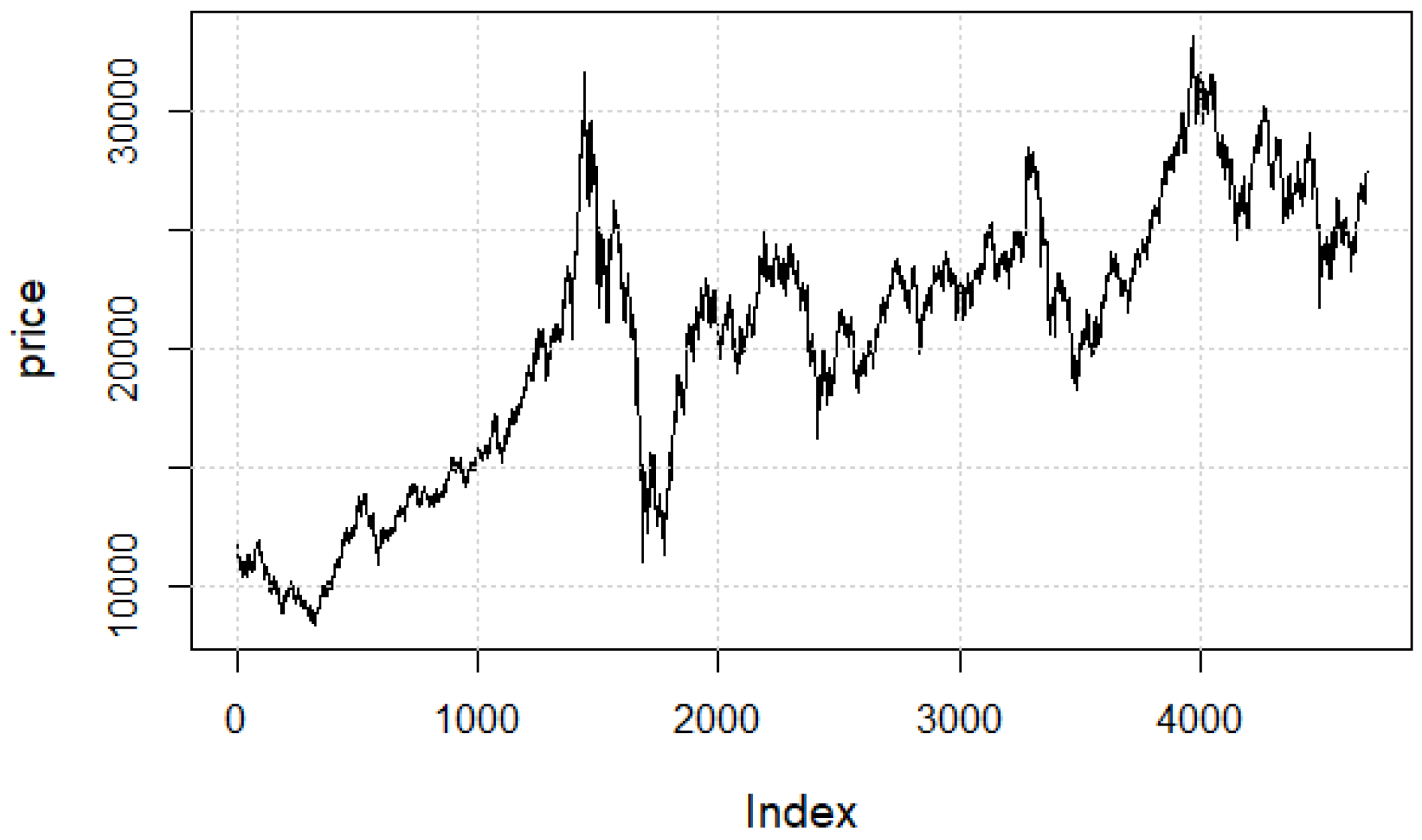
In this section, we will apply the proposed methodology to analyze the daily return series of Hong Kong Hang Seng Index (HSI). The data covers the periods from 2 January 2002 to 31 December 2020, which includes 4689 observations. The original series is shown in Figure 1. From Figure 1, we can clearly see that the daily price series is non-stationary. 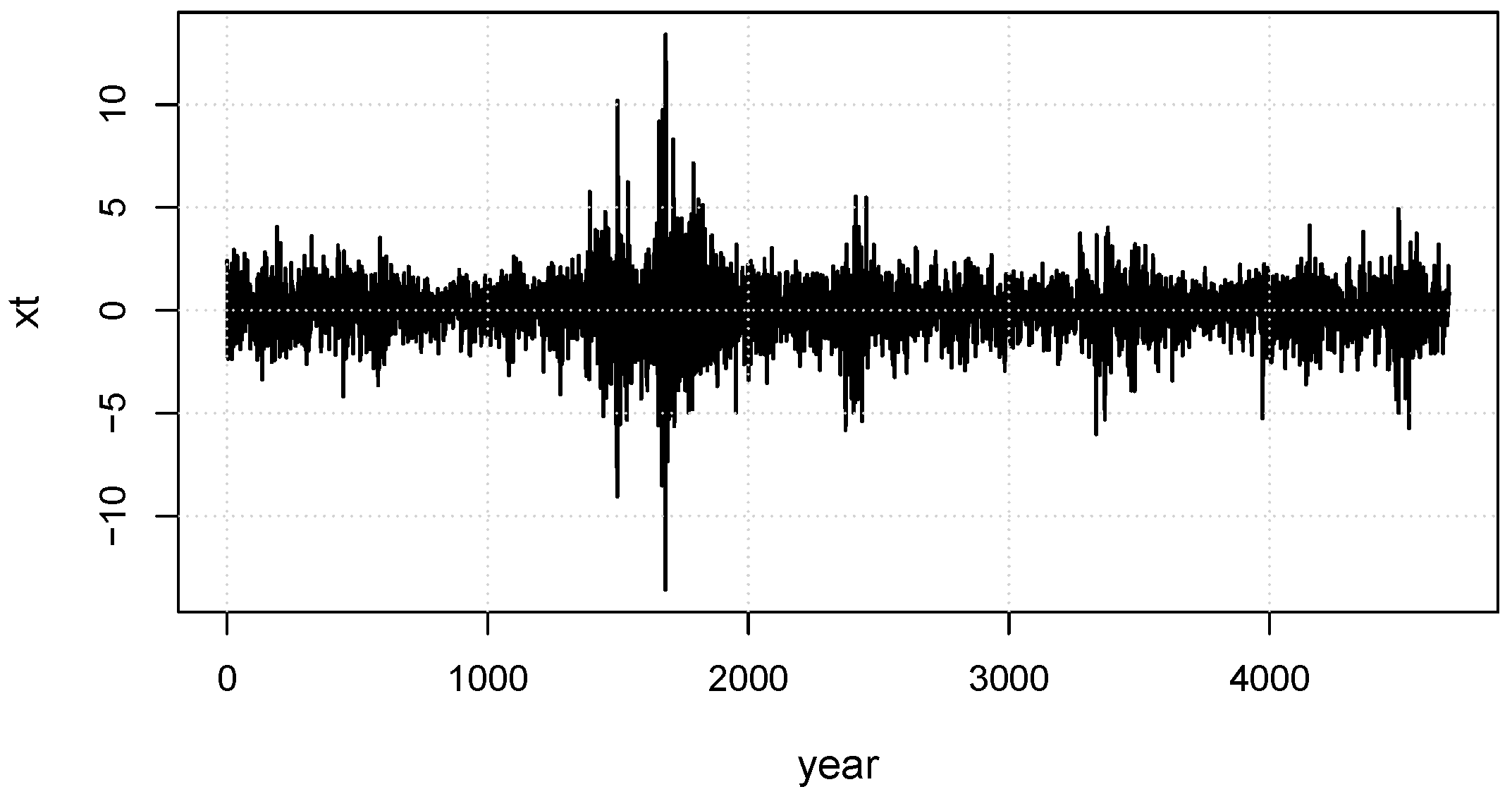Similar to [13], we let $x_t=100*(\log \left(P_t\right)-\log \left(P_{t-1}\right))$, where $P_t$ is the daily price in t-th day. The corresponding $x_t$ series are shown in Figure 2. We can observe from Figure 2 that $x_t$ is stationary. 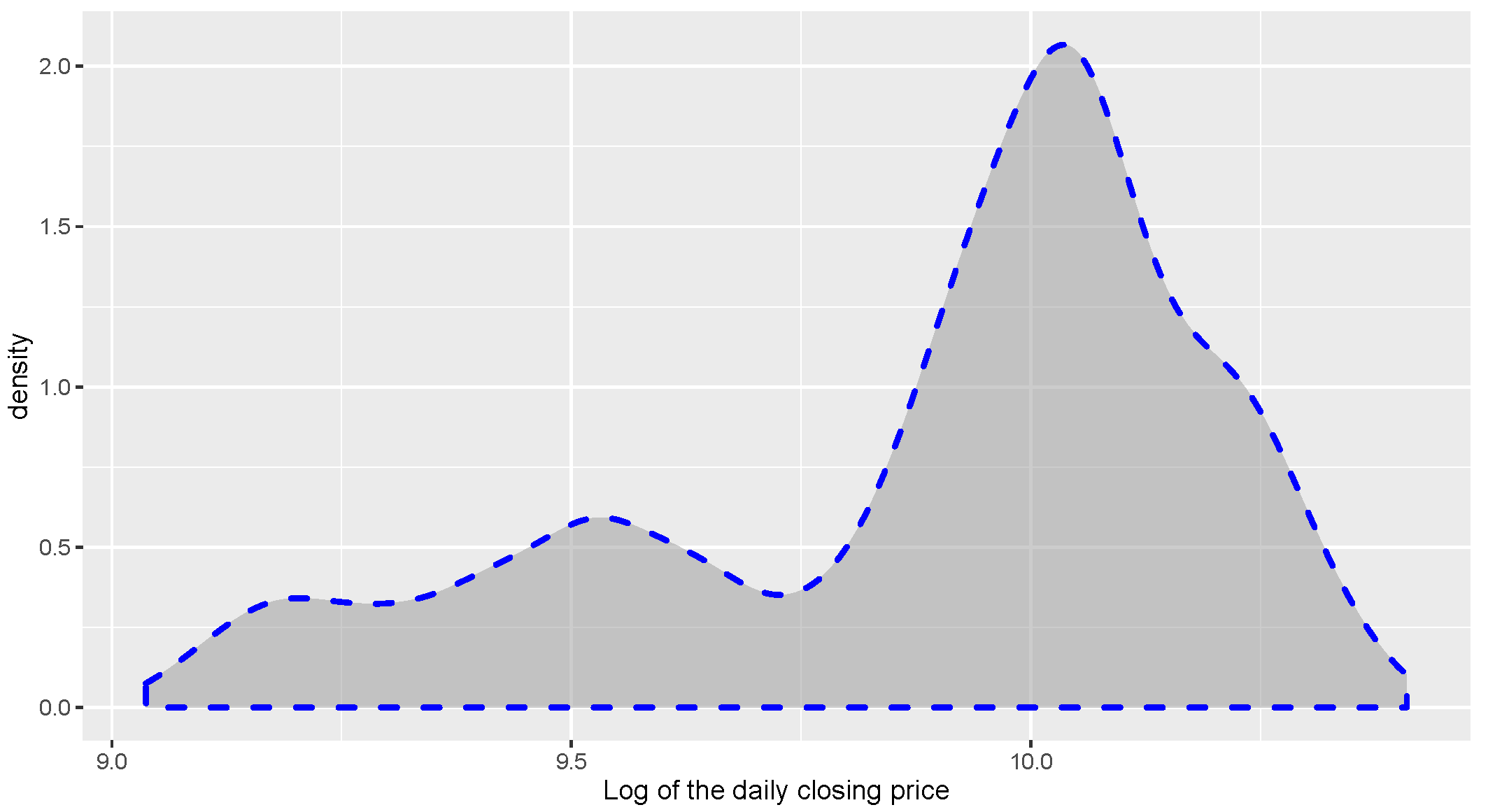The skewness and excess kurtosis of $x_t$ are −0.3 and 9.01, respectively, which also means that the $x_t$ series does not satisfy the normality assumption. Meanwhile, the density of log of the daily closing price of the Hong Kong Hang Seng Index is drawn in Figure 3. From Figure 3, we find that the marginal distribution of the series is clearly not symmetric and exhibits multimodality. This indicates that we need to use a mixture AR model rather than an AR model to describe the daily trend of HSI.

In real data analysis, it is important to choose the number of components k and the order of AR components for the MAR model. According to the distribution characteristics described above, we first consider a two-component mixture AR model and a three-component mixture AR model for this dataset. According to Wong & Li (2000) [1], we used AIC and BIC as the model-selection criteria. An example of the performances of the model-selection criteria can be seen in the Example 2 in Section 3.

The corresponding results are reported in

Table 9. AIC and BIC of a real dataset.

		$\mathbf{AR}\left(2\right)$		$\mathbf{AR}\left(3\right)$
Components	Method	AIC	BIC	AIC	BIC
	GMAR	5.86	70.38	9.86	87.29
k = 2	TMAR	5.79	70.32	9.80	87.23
	LMAR	5.80	70.33	9.79	87.22
	AEPD-MAR	5.61	70.14	9.62	87.06
	GMAR	15.82	112.61	21.82	137.97
k = 3	TMAR	15.76	112.56	21.74	137.90
	LMAR	15.76	112.55	21.75	137.90
	AEPD-MAR	15.68	112.48	21.68	137.83

. From Table 9, we can see that all of the methods rank the two-component as the best. Additionally, the best model selected by minimizing AIC and BIC is the two-component and second-order AEP-MAR model; the value of AIC is 5.61, and the value of BIC is 70.14. This shows that the AEP-MAR model can fit the characteristics of high kurtosis and multimodality in the the log-return series of HSI better. The estimation results for the selected model are given in

Table 10. The estimation results of two-component and second-order AEP-MAR model.

Component	${\mathit{\beta }}_1$	${\mathit{\beta }}_2$	$\mathit{\sigma }$	$\mathit{\tau }$	$\mathit{\alpha }$	$\mathit{\pi }$
component1	−0.0447	0.0610	0.5240	0.4808	1.2187	0.7564
component2	−0.6032	−0.1394	0.5473	0.5333	0.9012	0.2436

. According to Table 10, we obtain the following the two-component and second-order AEP-MAR model for the daily return series of Hong Kong Hang Seng Index.

$$\begin{array}{cc}\hfill h\left(x_t\right|{\mathcal{F}}_{t-1;}\mathit{\theta })=& 0.7564f_1\left(-0.0447x_{t-1}+0.0610x_{t-2},0.5240,1.2187,0.4808\right)\\ \hfill & +0.2436f_2\left(-0.6032x_{t-1}-0.1394x_{t-2},0.5473,0.9012,0.5333\right),\end{array}$$

(8)

We obtain from the model (8) that the first component can be interpreted as the overall trend of the log-returns with relatively small fluctuations, and the second component can be interpreted as the irrational “Unilateral Overshooting Phenomenon” in financial markets.

5. Discussion

In this paper, we introduced a robust mixture autoregressive procedure via an asymmetric exponential power distribution. The proposed method has greater flexibility and can adapt to unknown error structures. Under some specific parameters, our method can also be equivalent to the existing method, e.g., GMAR and LMAR as its special cases. In addition, an EM algorithm was introduced to solve the proposed optimization problem. The merits of the proposed method are illustrated by some numerical simulations and a real data analysis. The results indicated that the proposed method was robust and was adaptive to the error distribution. Finally, we will study the large sample properties of the proposed method as future work.

References

1. Wong, C.S.; Li, W.K. On a mixture autoregressive model. J. R. Stat. Soc. Ser. B 2000, 62, 95–115. [Google Scholar] [CrossRef]
2. Wong, C.S.; Chan, W.S.; Kam, P.L. A Student t-mixture autoregressive model with applications to heavy-tailed financial data. Biometrika 2009, 96, 751–760. [Google Scholar] [CrossRef]
3. Wong, C.S.; Li, W.K. On a mixture autoregressive conditional heteroscedastic model. J. Am. Stat. Assoc. 2001, 96, 982–995. [Google Scholar] [CrossRef]
4. Fong, P.W.; Li, W.K.; Yau, C.W.; Wong, C.S. On a mixture vector autoregressive model. Can. J. Stat. 2007, 35, 135–150. [Google Scholar] [CrossRef]
5. Nguyen, H.D.; McLachlan, G.J.; Ullmann, J.F.P.; Janke, A.L. Laplace mixture autoregressive models. Stat. Probab. Lett. 2016, 110, 18–24. [Google Scholar] [CrossRef]
6. Maleki, M.; Hajrajabi, A.; Arellano-Valle, R.B. Symmetrical and asymmetrical mixture autoregressive processes. Braz. J. Probab. Stat. 2020, 34, 273–290. [Google Scholar] [CrossRef]
7. Meitz, M.; Preve, D.; Saikkonen, P. A mixture autoregressive model based on Student’s t–distribution. Commun. Stat. Theory Methods 2021, 52, 1–76. [Google Scholar] [CrossRef]
8. Virolainen, S. A mixture autoregressive model based on Gaussian and Student’s t-distributions. Stud. Nonlinear Dyn. Econ. 2021, 26, 559–580. [Google Scholar] [CrossRef]
9. Solikhah, A.; Kuswanto, H.; Iriawan, N.; Fithriasari, K. Fisher’s z Distribution-Based Mixture Autoregressive Model. Econometrics 2021, 9, 27. [Google Scholar] [CrossRef]
10. Fernández, C.; Osiewalski, J.; Steel, M.F.J. Modeling and inference with υ-spherical distributions. J. Am. Stat. Assoc. 1995, 90, 1331–1340. [Google Scholar] [CrossRef]
11. Dempster, A.P.; Laird, N.M.; Rubin, D.B. Maximum likelihood from incomplete data via the EM algorithm. J. R. Stat. Soc. Ser. B 1977, 39, 1–22. [Google Scholar]
12. Yang, T.; Gallagher, C.M.; McMahan, C.S. A robust regression methodology via M-estimation. Commun. Stat. Theory Methods 2019, 48, 1092–1107. [Google Scholar] [CrossRef] [PubMed]
13. Chen, H.; Chong, T.T.-L.; Bai, J. Theory and applications of tar model with two threshold variables. Econ. Rev. 2012, 31, 142–170. [Google Scholar] [CrossRef] [Green Version]
Figure 1. The price of Hong Kong Hang Seng Index (HSI), January 2002–December 2020.
Axioms 12 00196 g001
Figure 2. The log-return of Hong Kong Hang Seng Index (HSI), January 2002–Dececember 2020.
Axioms 12 00196 g002
Figure 3. Density of log of the daily closing price of Hong Kong Hang Seng Index.
Axioms 12 00196 g003