Article

Mathematical Modeling of the Tumor–Immune System with Time Delay and Diffusion

1
School of Applied Mathematics, Dalian University of Technology, Dalian 116024, China
2
School of Software Technology, Dalian University of Technology, Dalian 116024, China
3
Department of Industrial Engineering, Institute of Maintenance and Industrial Safety, University of Oran 2 Mohamed Ben Ahmed, Oran 31000, Algeria
4
School of Advanced Control Technology, Dalian University of Technology, Dalian 116024, China
*
Authors to whom correspondence should be addressed.
Axioms 2023, 12(2), 184; https://doi.org/10.3390/axioms12020184
Submission received: 11 January 2023 / Revised: 7 February 2023 / Accepted: 8 February 2023 / Published: 10 February 2023

Abstract

:
This paper proposes a partial differential equation model based on the model introduced by V. A. Kuznetsov and M. A. Taylor, which explains the dynamics of a tumor–immune interaction system, where the immune reactions are described by a Michaelis–Menten function. In this work, time delay and diffusion process are considered in order to make the studied model closer to reality. Firstly, we analyze the local stability of equilibria and the existence of Hopf bifurcation by using the delay as a bifurcation parameter. Secondly, we use the normal form theory and the center manifold reduction to determine the normal form of Hopf bifurcation for the studied model. Finally, some numerical simulations are provided to illustrate the analytic results. We show how diffusion has a significant effect on the dynamics of the delayed interaction tumor–immune system.
MSC:
92D25; 92B05; 35K59; 37M10

1. Introduction

Some local tissue cells in the biological system lose their normal regulation or are infected by certain viruses in their growth and then become tumor cells. A primary cause of human death is malignant tumor cells. In order to minimize the possibility of a patient dying, it is necessary to use some specific treatments or a combination of therapies such as surgery, chemotherapy, radiotherapy, etc. However, the immune function of the body can inhibit the attack of normal cells by invaders and the transformation into potential cancer cells, which is a natural defense of biological organs against tumor growth [1]. For the early stages of cancer, the use of an immune response is effective to treat tumors [2,3]. Thus, immunotherapy is becoming an essential treatment for tumors [4]. Furthermore, the study of the dynamics of the tumor–immune interaction system by mathematical models is very important and is one of the biomedical models that has attracted considerable attention over the past few decades.
In order to understand the complex dynamics of the tumor–immune system, mathematical models, such as ordinary differential equations (ODEs) [5,6,7] and partial differential equations (PDEs) [8,9,10,11], are largely used to explore the dynamics of the immune system and tumor growth. Various valuable results have been achieved, and these results have an important theoretical and clinical meaning in tumor research. For example, in ref. [12], the authors present an analytic approach to describe and establish solutions to a porous medium system of equations, showing applications in invasive-invaded biological dynamics. Furthermore, interesting analytical results apropos invasive-invaded systems with nonlinear diffusion and advection are given in [13]. New results on the multidimensional stability of V-shaped traveling fronts for a reaction–diffusion equation with a nonlinear convection term in R n ( n 3 ) are presented in [14]. It is certain that constructing mathematical models supplies us with a new view to understanding the tumor–immune system.
Scientists have found that the immunity of an organism itself, which can help the immune cells fight against tumor cells, may be delayed [15]. Furthermore, resting cells can hunt and kill malignant tumor cells more than they can degenerate and transform into hunting cells themselves. Meanwhile, such a process can be achieved within a certain time interval, sometimes even a short time interval. Moreover, numerous scholars researching tumor–immune system interaction models have used only current information for predicting the future state [16,17]; however, future development not only depends on present information but also on past phenomena. For improving this issue, numerous scholars have considered the time delay in tumor–immune systems [18,19]. Ref. [20] considered a system of three-dimensional nonlinear delay differential equations, with the authors including time delay as a representation of the time lag for the conversion of resting cells to hunting cells. Ref. [21] studied the dynamics of tumor–immune system competition with time delay, and showed that the dynamical behavior of the system depends on the time delay parameter. Ref. [22] constructed a system of a number of immune cells that cooperate to protect the organs from tumor cells; the model included time delay to illustrate the activation process of immune cells. Ref. [23] proposed a Lotka–Volterra competition model with a step-wise constant delay to illustrate the interaction between tumor cells and T lymphocytes, and investigated the necessary and sufficient conditions for local and global stability.
The motivation for this paper is as follows. First, due to the processes of degeneration, proliferation, and transformation of tumor cells that can be achieved within a certain time interval, the existence of a time delay in the tumor–immune interaction system is necessary. Moreover, many scholars have shown that a time delay induces a change in the dynamical behavior of models, for example in [24,25], which can be biologically interpreted. Furthermore, the models governed by DDEs use past phenomena for predicting future information, which is more realistic. Second, the interaction between tumor cells and the immune system not only depends on time, but also on the space they live in. Moreover, tumor cells could spread in organs and trigger some factors, initiating the diffusion of tumor cells. Therefore, it is important to include time delay and diffusion into the tumor–immune interaction system, although investigating the time delay in specific mathematical models, such as models including spatial factors, is significant and more reasonable when we consider tumor–immune interaction problems. Third, Galach [26] analyzed a simplified version of Kuznetsov and Talyor’s model [27], where the immune reaction is described by a linear term, and then included the time delay in the interaction term between tumor cells and the immune system in the equation that describes the growth of tumor cells. However, the authors did not investigate the effect of time delay in Kuznetsov and Taylor’s model with the Michaelis–Menten function. Moreover, the diffusion of tumor cells and immune cells was not taken into account. Both immune and tumor reactions take a certain amount of time to identify alien cells and then react after a certain time delay.
Kuznetsov and Taylor’s model explains the response of effector cells to the growth of cancer cells; this model is different from other tumor–immune interaction system models because the authors consider the penetration of tumor cells by effector cells. Moreover, they use the Michaelis–Menten function to illustrate the production of tumor-specific immune cells. However, tumor invasion and metastatic spread are two essential and fundamental spatial processes that must be considered in such an important model. To establish the spatial effect issue, in this work, we consider Kuznetsov and Taylor’s model governed by PDEs, considering the time delay in the interaction term. Our model is the first to consider the time delay and diffusion process together in the original Kuznetsov and Taylor model (with the Michaelis–Menten function). In this paper, we analyze the stability equilibria to obtain the parameters that affect tumor growth and immune response the most. Moreover, we provide a detailed study to display the effect of diffusion parameters and time delay on the stability of equilibria and the occurrence of Hopf bifurcation.
This paper is organized as follows: We present a partial differential equation model with time delay and diffusion in Section 2. In Section 3, we carry out a qualitative analysis of the model, investigate the local stability of equilibria and detect the existence of Hopf bifurcation. In Section 4, by the use of the center manifold reduction method, we determine the normal form of Hopf bifurcation. We present some numerical simulations in Section 5. Finally, we present the conclusion of this study.

2. Model Formulation

The immune system contains many mechanisms for the identification and attack of tumor cells. The immune cells and tumor cells cannot recognize each other immediately, and there exists a time delay, τ , for responding. This response time may be small; however, it cannot be neglected. Furthermore, under the conditions of bounded resources and space, tumor cells and immune cells diffuse in the organs. Although the spatial environment affects the growth and interaction between tumor cells and immune cells, it does not only depend on time. Hence, it is also necessary to provide the complex interaction caused by spatial characteristics. Considering the above aspect, we construct the following system of non-linear equations governed by the partial differential equations in the presence of a time delay to study the dynamics of the tumor–immune interaction system:
u t ( x , t ) = c 1 Δ u ( x , t ) + α u ( 1 u ) c u ( t τ ) v ( t τ ) , t > 0 , x Ω , v t ( x , t ) = c 2 Δ v ( x , t ) β v + ζ u v η + u u ( t τ ) v ( t τ ) , t > 0 , x Ω , u x ( x , t ) = v x ( x , t ) = 0 , t 0 , x Ω u ( x , t ) = u 0 ( x , t ) 0 ; v ( x , t ) = v 0 ( x , t ) 0 t [ τ , 0 ] , x Ω ¯
where Ω is a bounded domain in R m ( m = 1 , 2 , 3 ) with smooth boundaries, Ω . For simplicity, we chose Ω = [ 0 , π ] , but all calculations can be extended for higher dimensions. u and v denote the density of cancer cells and immune cells at time t and location x . The descriptions of the parameters are given in Table 1.

3. Qualitative Analysis of the Model

3.1. Equilibria

In this section, we will find the positive steady states of model 1 which are biologically feasible. The steady state of model 1 is the solution of the system:
α u ( 1 u ) c u v = 0 , β v + ζ u v η + u u v = 0 ,
which are:
  • Free equilibrium (i.e., the absence of cancer cells and immune cells), E 0 = ( 0 , 0 ) .
  • The axial equilibrium (i.e., the cancer cells exist), E 1 = ( 1 , 0 ) .
  • The interior equilibrium (i.e., the coexistence of cancer cells and immune cells),
    E 2 = ( u * , v * ) = ( β + η ζ ) + ( β + η ζ ) 2 4 β η 2 , α c 2 ( β + η ζ ) + ( β + η ζ ) 2 4 η β 2 .
If ( H 2 ) β + η > ζ holds, then E 0 and E 1 are the only equilibria points. If ( H 1 ) β + η < ζ holds, then there is one interior equilibrium point, E 2 = ( u * , v * ) .

3.2. Stability and Bifurcation Analysis

To understand the dynamics of the suggested model and detect the effect of time delay and diffusion in the proposed model, we study the stability of equilibria and then we develop the bifurcation theory to describe how small parameters can change the qualitative behavior of the model.

3.2.1. Stability of E 0

The linearized system for model 1 about steady state E 0 has the form:
u ( x , t ) t = c 1 2 u ( x , t ) x 2 + α u ( x , t ) + h . o . t , v ( x , t ) t = c 2 2 v ( x , t ) x 2 β v ( x , t ) + h . o . t .
We can see that the linearized system is independent of the time delay; therefore, the stability of the equilibrium E 1 will depend only on the diffusion parameters.
We can investigate the stability of E 0 by substituting:
u ( x , t ) = cos ( n x ) u n ( x , t ) , v ( x , t ) = sin ( n x ) v n ( x , t ) , n = 0 , 1 , 2 ,
into the linearized system of model 1 to obtain the characteristic equation associated with E 0 as follows:
[ λ + c 1 n 2 α ] [ λ + c 2 n 2 + β ] = 0 .
Then, the stability result of the equilibrium E 0 is resumed in the following lemma.
Lemma 1.
Let c 1 * = α n 2 n = 0 , 1 , 2 , . The steady state E 0 is locally asymptotically stable for all τ 0 if c 1 > c 1 * , and is unstable if c 1 < c 1 * for all τ 0 .
Proof. 
The characteristic equation associated with equilibrium E 0 has two roots: λ 1 = c 2 n 2 β , which is always negative, and λ 2 = c 1 n 2 + α , which is negative if c 1 > α n 2 = c 1 * , ( n 0 ) and positive if c 1 < c 1 * for all τ 0 . If n = 0 (without diffusion), then the equilibrium E 0 is unstable for all τ 0 .
Remark 1.
The above result shows the necessity of including diffusion in the model; however, the diffusion parameters are responsible for the stability of the equilibrium E 0 .

3.2.2. Stability of E 1

We pass now to the stability analysis of the equilibrium E 1 to show the parameters that have an impact on the dynamics of the system.
The linearized system about the steady state E 1 = ( 1 , 0 ) has the form:
u ( x , t ) t = d 1 2 u ( x , t ) x 2 α u ( x , t ) c v ( x , t τ ) + h . o . t , v ( x , t ) t = d 2 2 v ( x , t ) x 2 β v ( x , t ) + ζ ( η + 1 ) 2 v ( x , t ) v ( x , t τ ) . x Ω , t > 0 .
The characteristic equation for τ = 0 is given by:
λ + d 1 n 2 + α λ + d 2 n 2 + β ζ η + 1 + 1 = 0 .
The characteristic equation above has two roots:
λ 1 = d 1 n 2 α < 0 ,
and
λ 2 = d 2 n 2 β + ζ η + 1 1 .
Under hypothesis ( H 2 ) , λ 2 is negative. Then, we have the stability results as follows.
Lemma 2.
When τ = 0 and ( H 2 ) holds, the steady state E 1 is locally asymptotically stable.

3.2.3. Stability and Bifurcation Analysis of the Interior Equilibrium

When ( H 1 ) holds, there exists an interior equilibrium. In what follows, we present the stability results for E 2 = ( u * , v * ) .
The characteristic equation around the equilibrium E 2 is given as follows:
λ 2 + A n λ + ( B n λ + C n ) e λ τ + F n = 0 ,
where A n , B n , C n and E n are given as follows:
A n = c 1 n 2 + c 2 n 2 α + 2 α u * + β ζ u * η + u * , B n = c v * + u * , C n = c v * c 2 n 2 + β ζ u * η + u * + u * α ( 2 u * 1 ) + c 1 n 2 u * + c u * ζ η v * ( η + u * ) 2 , F n = c 1 n 2 + 2 α u * α c 2 n 2 + β ζ u * η + u * .
For τ = 0 , the characteristic Equation (2) becomes:
λ 2 + ( A n + B n ) λ + C n + F n = 0 ,
with
A n + B n = c 1 n 2 + c 2 n 2 + α ( 2 u * 1 ) + c v 0 > α ( 2 u * 1 + c v * ) > 0 , C n + F n = c v * + c 1 n 2 + α ( 2 u * 1 ) c 2 n 2 + β ζ u * η + u * + u * α ( u * + v * ) + c 1 n 2 u * + c u * ζ η v * ( η + u * ) 2 .
Denote
Φ ( n ) = C n + F n = ϕ 2 n 4 + ϕ 1 n 2 + ϕ 0 ,
where
ϕ 2 = c 1 c 2 , ϕ 1 = c 1 β ζ u * η + u * + u * + c 2 ( c v * + α ( 2 u * 1 ) ) , ϕ 0 = u * α ( 2 u * 1 ) + c v * ζ η ( η + u * ) 2 + c v * + α ( 2 u * 1 ) β ζ u * η + u * .
Note that under the assumption ( H 3 ) α ( 2 u * 1 ) + c v * > 0 , ϕ 1 is positive. We are now able to formulate the next result.
Theorem 1.
For τ = 0 , the stability results for the system (1), when ( H 1 ) and ( H 3 ) hold, are given as follows:
  • If ϕ 0 < 0 , equilibrium E 2 is unstable.
  • If ϕ 0 > 0 and ϕ 1 ϕ 2 > 0 , equilibrium E 2 is locally asymptotically stable.
  • If ϕ 0 > 0 , ϕ 1 ϕ 2 < 0 , Φ ϕ 1 2 ϕ 2 > 0 and Φ ϕ 1 2 ϕ 2 + 1 > 0 , then the equilibrium E 2 is locally asymptotically stable.
  • If ϕ 0 > 0 , ϕ 1 ϕ 2 > 0 , Φ ϕ 1 2 ϕ 2 < 0 and Φ ϕ 1 2 ϕ 2 + 1 < 0 , then the equilibrium E 2 is unstable.
When τ > 0 , we suppose that ± i ω ( ω > 0 ) are a pair of purely imaginary roots of Equation (2), and by separating the real and imaginary parts we obtain:
ω 2 F n = C n c o s ω τ + B n ω s i n ω τ , A n ω = B n ω c o s ω τ C n s i n ω τ .
Thus,
cos ω τ = ( ω 2 F n ) C n A n B n ω 2 C n 2 + B n 2 ω 2 , sin ω τ = B n ω ( ω 2 F n ) + A n C n ω C n 2 + B n 2 ω 2 .
Which implies that
ω 4 + ( A n 2 B n 2 2 F n 2 ) ω 2 + F n 2 C n 2 = 0 .
Let ξ = ω 2 , then the above equation can be rewritten in the following form:
G ( ξ ) = ξ 2 + ( A n 2 B n 2 2 F n 2 ) ξ + F n 2 C n 2 .
The equation G ( ξ ) = 0 :
  • Has no positive roots if ( H 4 ) : A n 2 B n 2 2 F n 2 < 0 .
  • Has one unique positive root, ω 0 , if ( H 5 ) : F n 2 C n 2 < 0 holds.
  • Has two positive roots, ω 1 , 2 , if ( H 6 ) : A n 2 B n 2 2 F n 2 < 0 , F n 2 C n 2 > 0 , ( A n 2 B n 2 2 F n 2 ) 2 4 ( F n 2 C n 2 ) 2 > 0 holds.
If the assumption ( H 6 ) holds, then the critical time delay is determined as follows:
τ l ( k ) = 1 ω l arccos ( ω l 2 F n ) C n A n B n ω l 2 C n 2 + B n 2 ω l 2 + 2 k π , if ( ω l 2 F n ) C n A n B n ω l 2 > 0 , 1 ω l 2 π arccos ( ω l 2 F n ) C n A n B n ω l 2 C n 2 + B n 2 ω l 2 + 2 k π , if ( ω l 2 F n ) C n A n B n ω l 2 < 0 , for l = 0 , 1 , 2 k = 0 , 1 , 2 , .
Now, the transversality conditions yield:
d λ d τ τ = τ l ( k ) 1 = ( 2 λ + A n ) e λ τ λ ( B n λ + C n ) + B n λ ( B n λ + C n ) = ξ F n 2 ξ + B n 2 ξ 2 G ( ξ ) . l = 0 , 1 , 2 ; k = 0 , 1 , 2 , .
This will signify that at least one eigenvalue exists with a non-negative real part for τ > τ l ( k ) . Furthermore, the conditions for the existence of Hopf bifurcation are necessary to prove that periodic solutions exist.
Theorem 2.
For system (1), τ > 0 . If the hypotheses ( H 1 ) and ( H 3 ) hold, and the stability conditions of Theorem 1 hold, then:
  • If ( H 4 ) is satisfied, then E 2 is locally asymptotically stable for all τ > 0 .
  • If ( H 5 ) is satisfied, then E 2 is locally asymptotically stable for 0 < τ < τ 0 0 and unstable for τ > τ 0 0 , and the system undergoes a Hopf bifurcation at τ = τ 0 ( k ) and k = 0 , 1 , 2 , .
  • If ( H 6 ) is satisfied, then there exists m N such that:
    (a)
    E 2 is locally asymptotically stable if τ [ 0 , τ 2 ( 0 ) ) j = 0 m 1 ( τ 1 ( j ) , τ 2 ( j + 1 ) ) .
    (b)
    E 2 is unstable if τ j = 0 m 1 ( τ 2 ( j ) , τ 1 ( j ) ) ( τ 2 ( m ) , + ) .
    (c)
    System (1) undergoes a Hopf bifurcation at E 2 when τ = τ l ( k ) , l = 1 , 2 , and k = 0 , 1 , 2 , .
Remark 2.
If ( H 1 ) holds, then the stability analysis for the equilibrium E 1 and E 2 in the presence of time delay τ are similar.

4. Normal Form of Hopf Bifurcation

In this section, we try to derive the normal formal of Hopf bifurcation at the interior equilibrium E 2 = ( u * , v * ) when τ 0 for the system (1). We define u ¯ ( x , t ) = u ( x , t ) u * and v ¯ ( x , t ) = v ( x , t ) v * . Herein, we have omitted the bar for convenience. The system (1) is then given by:
u ( x , t ) t = τ [ c 1 2 u ( x , t ) x 2 + α u ( x , t ) ( 1 u ( x , t ) 2 u * ) c u ( x , t 1 ) v ( x , t 1 ) + u * v ( x , t 1 ) + v * u ( x , t 1 ) ] , v ( x , t ) t = τ [ c 2 u ( x , t ) t β v ( x , t ) + ζ η + u * + u ( x , t ) u ( x , t ) u * + u ( x , t ) v * + u ( x , t ) v ( x , t ) u ( x , t 1 ) v ( x , t 1 ) + u * v ( x , t 1 ) + v * u ( x , t 1 ) v * u ( x , t ) β + u * η + u * + u ( x , t ) ] . u ( x , t ) t = v ( x , t ) x = 0 , t 0 , x Ω , u ( x , t ) = u 0 ( x , t ) 0 ; v ( x , t ) = v 0 ( x , t ) 0 , t [ τ , 0 ] , x Ω ¯ .
Let h = ( h 11 , h 12 ) T be the eigenvector of the linear operator corresponding to eigenvalue i ω τ , < h * ¯ , h > = h * ¯ T . h = 1 , where h * = ( h 21 , h 22 ) T is the normalized eigenvector of the adjoint operator of the linear operator corresponding to the eigenvalues i ω τ . We then obtain:
h = ( h 11 , h 12 ) T = 1 , ζ η + u * v * c u * T , h * = ( h 21 , h 22 ) T = d i ω c 2 n 2 β + ζ η + u * u * c u * , 1 T , d = i ω c 2 n 2 β + ζ η + u * u * c u * + ζ η + u * v * i ω + c 2 n 2 + β ζ η + u * u * 1 .
Let
U ( x , t ) = U ( x , T 0 , T 1 , T 2 , ) = k = 1 + ϵ k U k ( x , T 0 , T 1 , T 2 , )
be the solution to Equation (7), where
U ( x , T 0 , T 1 , T 2 , ) = ( u ( x , T 0 , T 1 , T 2 , ) , v ( x , T 0 , T 1 , T 1 , ) ) T , U k ( x , T 0 , T 1 , T 2 , ) = ( u k ( x , T 0 , T 1 , T 1 , ) , v k ( x , T 0 , T 1 , T 2 , ) ) T .
Denote D i = T i , i = 0 , 1 , 2 , and
d d t = T 0 + ϵ T 1 + ϵ 2 T 2 + = D 0 + ϵ D 1 + ϵ 2 D 2 + , u j = u j ( x , T 0 , T 1 , T 2 , ) , u j , 1 = u j ( x , T 0 1 , T 1 , T 2 , ) , v j = v j ( x , T 0 , T 1 , T 2 , ) , v j , 1 = v j ( x , T 0 1 , T 1 , T 2 , ) . j = 1 , 2 , 3 , .
We then have
d U ( x , t ) d t = ϵ D 0 U 1 + ϵ 2 D 0 U 2 + ϵ 3 D 1 U 1 + ϵ 3 D 0 U 3 + ϵ 3 D 1 U 2 + ϵ 3 D 2 U 1 + , 2 U ( x , t ) x 2 = ϵ 2 U 1 x 2 ( x , t ) + ϵ 2 2 U 2 x 2 ( x , t ) + ϵ 3 2 U 3 x 2 ( x , t ) + .
We take perturbation τ = τ ϵ + ϵ + μ to deal with the delayed terms, we expand U ( x , t 1 ) and v ( x , t 1 ) at u ( x , T 0 1 , T 1 , T 2 , ) and v ( x , T 0 1 , T 1 , T 2 , ) , respectively; that is,
u ( x , t 1 ) = ϵ u 1 , 1 + ϵ 2 u 2 , 1 ϵ 3 D 1 u 1 , 1 + ϵ 3 u 3 , 1 ϵ 3 D 1 u 2 , 1 ϵ 3 D 2 u 1 , 1 + , v ( x , t 1 ) = ϵ v 1 , 1 + ϵ 2 v 2 , 1 ϵ 2 D 1 v 1 , 1 + ϵ 3 v 3 , 1 ϵ 3 D 1 v 2.1 ϵ 3 D 2 v 1 , 1 + ,
where u j , 1 = u j ( x , T 0 1 , T 1 , T 2 , ) , v j , 1 = v j ( x , T 0 1 , T 1 , T 2 , ) and j = 1 , 2 , 3 , . Substituting (9) and (13) into Equation (7), for the ϵ -order terms, we obtain:
D 0 u 1 τ ϵ c 1 2 U 1 x 2 τ ϵ α u 1 + 2 τ ϵ α u 1 u * + c τ ϵ ( u * v 1 , 1 + v * u 1 , 1 ) = 0 , D 0 v 1 τ ϵ c 2 2 v 1 x 2 + τ ϵ β v 1 ϵ τ ϵ u * + u 1 + η ( u 1 u * + u 1 v * ) + τ ϵ ( u * v 1 , 1 + v * u 1 , 1 ) v * τ ϵ u 1 β + u * η + u * + u 1 = 0 .
Since ± i ω τ are the eigenvalues of the linear part of (7), the solution to (14) can be expressed in the following form:
U 1 ( x , T 0 , T 1 , T 2 , ) = F ( T 1 , T 2 , ) e i ω τ ϵ T 0 h cos ( n x ) + r e s t ,
where r e s t means the conjugate of the preceding terms and h is given in (8) . For the ϵ 2 order terms, we obtain:
D 0 u 2 τ ϵ c 1 2 u 2 x 2 τ ϵ α u 2 + 2 τ ϵ α u * u 2 + c τ ϵ ( u * v 2 , 1 + u 2 , 1 v * ) = D 1 u 1 + μ c 1 2 u 1 x 2 + μ α u 1 2 μ α u * u 1 + c ( τ ϵ D 1 v 1 , 1 τ ϵ v 1 v 1 , 1 μ u * v 1 , 1 + τ ϵ u 1 u 1 , 1 μ v * u 1 , 1 ) , D 0 v 2 τ ϵ c 2 2 v 2 x 2 + τ ϵ β v 2 ζ τ ϵ u * + u 2 + η ( u 2 v * + v 2 u * ) v * u 2 β + u * η + u * + u 2 = D 1 v 1 + μ c 2 2 v 1 x 2 μ β v 1 + ζ τ ϵ u * + u 1 + η ( τ ϵ u 1 v 1 + μ u * v 1 + μ v * u 1 ) ( τ ϵ c 1 u * v 1 , 1 τ ϵ v 1 v 1 , 1 μ u * v 1 , 1 + τ ϵ D 1 v * u 1 , 1 τ ϵ u 1 u 1 , 1 μ v * u 1 , 1 ) + μ v * u 1 ζ u * η + u * + u 1 .
We substitute Equation (16) into (15), we obtain the coefficient vector of term e i ω τ ϵ T 0 , then we obtain:
d c d T 1 = M μ F
where
M = h 12 ¯ h 11 ( v * n 2 c 1 u * e i ω τ ϵ u * α ) c u * h 21 ¯ h 12 h 22 ¯ h 11 ζ u * η + u * ( h 11 h 21 ¯ + h 12 h 22 ¯ ) α u * τ ϵ h 11 h 21 ¯ e i ω τ ϵ .
Suppose that the solution of Equation (16) is
u 2 = k = 0 + r 0 k F F ¯ + r 1 k F 2 e 2 i ω τ ϵ T 0 + r 1 k ¯ G ¯ 2 e 2 i ω τ ϵ T 0 cos ( k x ) , v 2 = k = 0 + m 0 k F F ¯ + m 1 k F 2 e 2 i ω τ ϵ T 0 + m 1 k ¯ F ¯ e 2 i ω τ ϵ T 0 cos ( k x ) ,
where
r 0 k = p k G 2 k c 1 + u * ζ u * η + u * 1 h 11 h 12 ¯ + h 12 h 11 ¯ + 2 c e i ω τ ϵ h 11 h 11 ¯ c 2 k 2 β u * + ζ u * η + u * , m 0 k = p k G 2 k c h 11 + h 12 ¯ 2 e i ω τ ϵ ζ u * η + u * v * + ( h 11 h 12 ¯ + h 12 h 11 ¯ ) c ζ u * η + u * 1 ( c 1 k 2 + α u * + α + v * c ) , r 1 k = p k G 1 k c e i ω τ ϵ h 11 2 + α h 11 h 12 c 2 k 2 + 2 i ω + ζ u * u * + η β u * + α ζ u * η + u * 1 h 11 h 12 , m 1 k = p k G 1 k 2 i ω + c 1 k 2 + α u * + α + c u * e 2 i ω τ ϵ ζ u * u * + η 1 h 11 h 12 v * ζ u * u * + η 1 c e i ω τ ϵ h 11 2 + α h 11 h 12 ,
with
p k = < cos ( n x ) cos ( n x ) , cos ( k x ) > = 0 π cos ( n x ) cos ( n x ) cos ( k x ) d x .
F 1 k = 2 i α ω + c 1 k 2 + α u * + α + v * c e 2 i ω τ ϵ 2 i ω + c 2 k 2 + u * η + u * β u * + c ζ v * ( η + u * ) 2 0 π cos ( k x ) cos ( k x ) d x , F 2 k = c v * u * ζ η + u * + c 2 k 2 + u * η + u * β u * c 1 k 2 + α u * + α + c v * .
For the ϵ 3 order terms, we obtain:
D 0 u 3 τ ϵ c 1 2 u 3 x 2 τ ϵ α u 3 + 2 τ ϵ α u 3 + c τ ϵ ( u * v 3 + u 3 v * ) = D 1 u 2 D 2 u 1 + μ c 1 2 u 2 x 2 + μ α u 2 2 μ α u 2 + c τ ϵ ( D 1 u 2 , 1 + D 2 u 1 , 1 v 1 v 2 , 1 v 2 v 1 , 1 ) c μ ( u * v 2 , 1 u * D 1 v 1 , 1 + v 1 v 1 , 1 ) c τ ϵ ( u 2 v 1 + u 1 v 2 ) c μ ( u 1 v 1 + u * v 2 + v * u 2 ) , D 0 v 3 τ ϵ c 2 2 v 3 x 2 τ ϵ β v 3 ζ τ ϵ u * + u 3 + η ( u 3 v * + v 3 u * ) v * u 3 ζ u * η + u * + u 3 = D 1 v 2 D 2 v 1 + μ c 2 2 v 3 x 2 β μ v 2 + ζ τ ϵ u * + u 2 + η ( u 2 v 1 + v 2 u 1 ) + ζ μ u * + u 2 + η ( u 1 v 1 + u * v 2 + v * u 2 ) + τ ϵ ( D 2 c 1 u * v 1 , 1 + D 1 u * v 2 , 1 v 1 v 2 , 1 + D 1 v 1 v 1 , 1 ) μ ( v * v 2 , 1 v * D 1 v 1 , 1 v 1 v 1 , 1 ) .
We substitute Equations (15) and (17) into Equation (18), we obtain the coefficient vector of term e i ω τ ϵ T 0 , then we obtain:
F T 2 = Ξ F 2 F ¯ ,
with
Ξ = 1 G 3 α τ ϵ h 21 ¯ k 0 ( d k r 0 k h 11 + h 11 ¯ r 0 k e 2 i ω τ ϵ + r 0 k h 11 e i ω τ ϵ + r 1 k h 11 ¯ e i ω τ ϵ ) + h 22 ¯ ζ e t a + u * τ ϵ k 0 d k ( r 0 k h 12 r 1 k h 12 ¯ + m 0 k h 11 + m 1 k h 11 ¯ )
and
G 3 = h 21 ¯ ( h 11 c u * τ ϵ h 11 e i ω τ ϵ ) + h 22 ¯ h 12 0 π cos ( π x ) cos ( n x ) d x .
In conclusion, the normal form of Hopf bifurcation for the system (1) reduced on the center manifold is
F T = ϵ F T 1 + ϵ 2 F T 2 + .
Let F F ϵ ; thus, the above equation becomes:
F = M μ F + Ξ F 2 F ¯ .
To obtain the normal form of Hopf bifurcation in polar coordinates, we let F = r e i θ , we thus obtain:
r ˙ = ( M ) μ r + ( Ξ ) r 3 , θ ˙ = ( M ) μ + ( Ξ ) r 2 .
.
We state the following theorem.
Theorem 3.
If ( M ) μ ( Ξ ) holds for system (19), system (1) admits periodic solutions around the positive equilibrium.
  • If ( M ) μ < 0 , the bifurcating periodic solutions are unstable.
  • If ( M ) μ > 0 , the bifurcating periodic solutions are locally asymptotically stable.

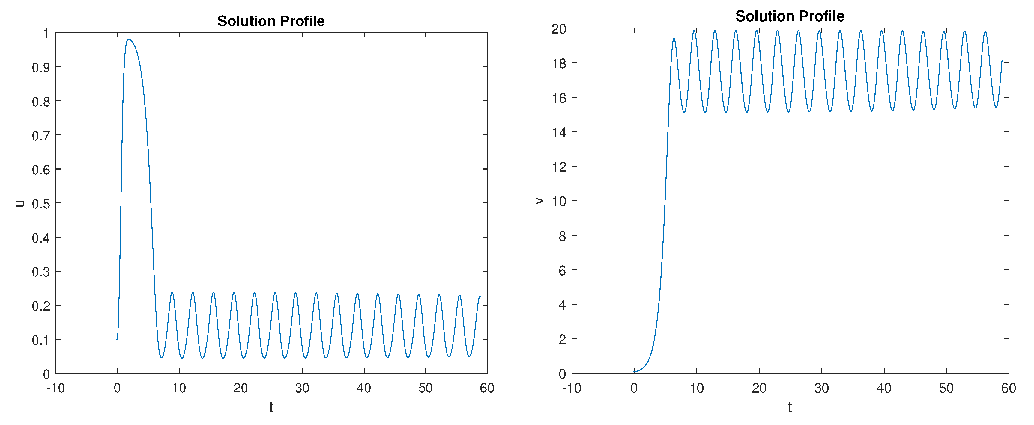
5. Numerical Simulations

This part is devoted to the exposition of the results throughout numerical simulations. The values of parameters are chosen according to [27] and are stated in Table 2.
Remark 3.
The numerical simulations in this paper were carried out using the software Matlab and were performed over a spatial domain [ 0 , π ] and over a time domain [ 0 , 100 ] . Most of the parameters are as described in the Table 1. In the absence of delay (i.e., τ = 0 ), the "built-in pdepe" function was used to plot the results. We provide both the spatial patterns of the solutions in addition to solution profiles for t [ 0 , 100 ] . When the time delay was positive (i.e., τ > 0 ), numerical simulations were obtained using a forward-in-time and centered-in-space finite differences scheme. The spatial mesh interval was Δ x = 0.03 and the time step was Δ t = 0.01 .

Discussion

When τ = 0 and η = 4.5 , we have β + η > ζ . Then, the hypothesis ( H 2 ) holds. According to Lemma 2, E 1 = ( 1 , 0 ) is locally asymptotically stable, which is shown in Figure 1. For τ = 0 , the positive equilibrium E 2 is locally asymptotically stable, Figure 2, and for τ = 0.19 > τ 0 0 , E 2 loses its stability and we observe that Hopf bifurcation occurs, Figure 3. With the set of values given in Table 1, the hypothesis ( H 1 ) holds, then the system (1) admits a unique positive equilibrium point E 2 = ( 0.1 , 18 ) T . We have F 0 2 C 0 2 = 6142.23 < 0 , then ( H 5 ) holds, and the stability of the interior steady state is determined by τ according to Theorem 2, i.e., E 2 is locally asymptotically stable if τ ( 0 , τ 0 0 ) , whereas E 2 is unstable if τ > τ 0 0 . With same set of values, we obtain ω 0 = 20.317 and τ 0 0 = 0.02 as the solutions of Equations (5) and (6), respectively. Therefore, we depict some spatiotemporal patterns for this case by taking τ as a varying parameter and initial conditions of ( u ( t ) , v ( t ) ) = ( 0.1 , 0.1 ) for t [ τ , 0 ] .
Observing the figures of the numerical simulations with a time delay and in the absence of a time delay, we notice that when the time delay is inferior to the critical value, the interior equilibrium is locally asymptotically stable, which means that the immune system can keep tumor cell growth under control at this moment. Tumor cells may not proliferate extensively in the organs. It is established that the immune and tumor cells could coexist in the body. Although the efficiency of the immune system is shown (see Figure 2 and Figure 4), as the time delay increases, periodic variation is observed (Figure 3 and Figure 5). This demonstrates that the hyperplasia time for tumor cells is large, which diminishes the efficiency of the immune system.

6. Conclusions

In this work, we explore a mathematical model which explains the tumor–immune interaction system. The model which refers to Kuznetsov–Taylor’s model with the Michaelis–Menten function is based on partial differential equations with a time delay. First, we investigate the stability of the equilibria in the absence of a time delay. Using the time delay as a bifurcation parameter, the necessary conditions for the stability of the interior equilibrium in the presence of a time delay are established. The critical value for which Hopf bifurcation occurs is obtained. We show that when the bifurcation parameter, τ , passes through the critical value, the stability of an interior equilibrium changes from stable to unstable. Applying the normal form together with the center manifold reduction, the normal form of Hopf bifurcation of the considered model is determined. In this paper, we consider spatial factors and the essential time for the reaction of the immune system and the tumor cells; then, by analysis of the results and numerical simulations, we observe that the critical value of Hopf bifurcation depends on diffusion. The stability of bifurcating periodic solutions can be also changed. Therefore, the dynamical behavior of the tumor–immune interaction system can be affected by spatial factors and time delay.

Author Contributions

Methodology, A.C.; software, A.M.-K.; formal analysis, A.C.; investigation, A.M.-K.; writing—original draft, A.C.; writing—review and editing, M.H.; supervision, M.L.; project administration, M.L.; funding acquisition, A.C. All authors have read and agreed to the published version of the manuscript.

Funding

This research received no external funding.

Institutional Review Board Statement

Not applicable.

Informed Consent Statement

Not applicable.

Data Availability Statement

Not applicable.

Acknowledgments

We would like to thank the editors and reviewers for taking the time and effort to review the manuscript. We sincerely appreciate all valuable comments and suggestions, which helped us to improve the quality of the manuscript.

Conflicts of Interest

The authors declare no conflict of interest.

Abbreviations

The following abbreviations are used in this manuscript:
ODEsOrdinary differential equations
DDEsDelay differential equations
PDEsPartial differential equations

References

  1. Eckert, A.W.; Wickenhauser, C.; Salins, P.C.; Kappler, M.; Bukur, J.; Seliger, B. Clinical relevance of the tumor microenvironment and immune escape of oral squamous cell carcinoma. J. Transl. Med. 2016, 14, 85. [Google Scholar] [CrossRef] [PubMed]
  2. Shi, X.; Cheng, Q.; Hou, T.; Han, M.; Smbatyan, G.; Lang, J.E.; Epstein, A.L.; Lenz, H.J.; Zhang, Y. Genetically Engineered Cell-Derived Nanoparticles for Targeted Breast Cancer Immunotherapy. Mol. Ther. 2020, 28, 536–547. [Google Scholar] [CrossRef] [PubMed]
  3. Bidmon, N.; Kind, S.; Welters, M.; Joseph-Pietras, D.; Laske, K.; Maurer, D.; Hadrup, S.R.; Schreibelt, G.; Rae, R.; Sahin, U. Development of an RNA-based kit for easy generation of TCR-engineered lymphocytes to control T-cell assay performance. J. Immunol. Methods 2018, 458, 74–82. [Google Scholar] [CrossRef] [PubMed]
  4. Berzofsky, J.A.; Terabe, M.; Oh, S.; Belyakov, I.M.; Ahlers, J.D.; Janik, J.E.; Morris, J.C. Progress on new vaccine strategies for the immunotherapy and prevention of cancer. J. Clin. Investig. 2004, 113, 1515–1525. [Google Scholar] [CrossRef]
  5. Frhlich, F.; Loos, C.; Hasenauer, J. Scalable Inference of Ordinary Differential Equation Models of Biochemical Processes. In Gene Regulatory Networks: Methods and Protocols; Humana Press: New York, NY, USA, 2019. [Google Scholar]
  6. Xla, D.; Dwa, B.; Pza, B.; Yla, C. Recent advances in nanosized drug delivery systems for overcoming the barriers to anti-PD immunotherapy of cancer. Nano Today 2019, 29, 100801. [Google Scholar]
  7. Lai, X.; Friedman, A. Combination therapy of cancer with cancer vaccine and immune checkpoint inhibitors: A mathematical model. PLoS ONE 2017, 12, e0178479. [Google Scholar] [CrossRef]
  8. Wu, K.; Xiu, D. Data-Driven Deep Learning of Partial Differential Equations in Modal Space. J. Comput. Phys. 2020, 408, 109307. [Google Scholar] [CrossRef]
  9. Pettet, G.J.; Please, C.P.; Mcelwain, M. The migration of cells in multicell tumor spheroids. Bull. Math. Biol. 2001, 63, 231–257. [Google Scholar] [CrossRef]
  10. López, L.; Seoane, J.M.; Sanjuán, M. Dynamics of the cell-mediated immune response to tumour growth. Philos. Trans. R. Soc. A Math. Phys. Eng. Sci. 2017, 375, 20160291. [Google Scholar] [CrossRef]
  11. Kayan, E.; Merdan, H. An algorithm for Hopf bifurcation analysis of a general delayed reaction-diffusion model. Nonlinear Dyn. 2016, 89, 345–366. [Google Scholar] [CrossRef]
  12. Palencia, J.; González, J.; Rahman, S.U.; Redondo, A.N. Regularity, Asymptotic Solutions and Travelling Waves Analysis in a Porous Medium System to Model the Interaction between Invasive and Invaded Species. Mathematics 2022, 10, 1186. [Google Scholar] [CrossRef]
  13. Palencia, J. Invasive-invaded system of non-Lipschitz porous medium equations with advection. Int. J. Biomath. 2021, 14, 2150061. [Google Scholar] [CrossRef]
  14. Niu, H.L. Multidimensional stability of V-shaped traveling fronts in bistable reaction-diffusion equations with nonlinear convection. AIMS Math. 2021, 6, 314–332. [Google Scholar] [CrossRef]
  15. Chen, M.L. Dynamics of a HIV Infection Model with Delay in Immune Response. J. Biomath. 2009. [Google Scholar]
  16. Eladdadi, A.; Kim, P.; Mallet, D. Mathematical Models of Tumor-Immune System Dynamics; Springer: New York, NY, USA, 2014. [Google Scholar]
  17. D’Onofrio, A. Tumor-immune system interaction: Modeling the tumor-stimulated proliferation of effectors and immunotherapy. Math. Models Methods Appl. Sci. 2006, 16, 1375–1401. [Google Scholar] [CrossRef]
  18. Xie, J.H.; Zhao, T.J.; Hao, F.F.; He, F.; Science, S.O. The effect of time delay on tumor-immune system during tumor growth. J. Med. Biomech. 2017, 32, 319–324. [Google Scholar]
  19. Dong, Y.; Huang, G.; Miyazaki, R.; Takeuchi, Y. Dynamics in a tumor immune system with time delays. Appl. Math. Comput. 2015, 252, 99–113. [Google Scholar] [CrossRef]
  20. Babushkina, N.A.; Kuzina, E.A. Mathematical Modeling of Antitumor Viral Vaccine Therapy: From the Experiment to the Clinic. Adv. Syst. Sci. Appl. 2020, 20, 1–23. [Google Scholar]
  21. Yafia, R. Hopf bifurcation in a delayed model for tumor-immune system competition with negative immune response. Discret. Dyn. Nat. Soc. 2006, 2006, 095296. [Google Scholar] [CrossRef]
  22. Yusnaeni, A.; Kasbawati, K.; Syamsuddin, T. Analytical Study of the Existence of a Hopf Bifurcation in the Tumor Cell Growth Model with Time Delay. InPrime: Indonesian J. Pure Appl. Math. 2021, 3, 20–28. [Google Scholar] [CrossRef]
  23. Gurcan, F.; Kartal, S.; Ozturk, I.; Bozkurt, F. Stability and bifurcation analysis of a mathematical model for tumor-immune interaction with piecewise constant arguments of delay. Chaos Solitons Fractals 2014, 68, 169–179. [Google Scholar] [CrossRef]
  24. Sardar, M.; Khajanchi, S.; Biswas, S.; Abdelwahab, S.F.; Nisar, K.S. Exploring the dynamics of a tumor-immune interplay with time delay. AEJ—Alexandria Eng. J. 2021, 60, 4875–4888. [Google Scholar] [CrossRef]
  25. Soufiani, B.N.; Salamci, M.U. Effect of Delay of Immune System Response in Cancer Dynamics: Bifurcation and Chaos Analysis. In Proceedings of the 2018 26th Mediterranean Conference on Control and Automation (MED), Zadar, Croatia, 19–22 June 2018; pp. 765–770. [Google Scholar]
  26. Gaach, M. Dynamics of the tumor-immune system competition: The effect of time delay. Int. J. Appl. Math. Comput. Sci. 2003, 13, 395–406. [Google Scholar]
  27. Kuznetsov, V.A.; Makalkin, I.A.; Taylor, M.A.; Perelson, A.S. Nonlinear dynamics of immunogenic tumors: Parameter estimation and global bifurcation analysis. Bull. Math. Biol. 1994, 56, 295–321. [Google Scholar] [CrossRef] [PubMed]
Figure 1. Mesh plot formation of solution of the system (1) in the absence of a time delay (a,b) and corresponding solution profile plots formation (c,d). Here, the parameters are as in Table 2, except that η = 4.5 .
Axioms 12 00184 g001
Figure 2. Mesh plot formation of the solutions of the system (1) in the absence of a time delay. (a,b) represent the solutions u and v respectively.
Axioms 12 00184 g002
Figure 3. Mesh plot formation of solution of the system (1) in the presence of a time delay (a,b) and spatiotemporal pattern formation (c,d).
Axioms 12 00184 g003
Figure 4. Solutions profile shapes of system (1) in the absence of a delay.
Axioms 12 00184 g004
Figure 5. Solutions profile shapes of system (1) in the presence of a time delay.
Axioms 12 00184 g005
Table 1. Descriptions of the parameters of model (1).
ParametersDescription
c 1 Diffusion rate of cancer cells
c 2 Diffusion rate of immune cells
α The growth rate of cancer cells
c The coefficient of interaction between
immune cells and tumor cells
ζ The production rate of immune cells
stimulated by cancer cells
β The natural death rate of immune cells
η The number of cancer cells by which
the immune system responds is half of its maximum
τ The discrete time delay in interconnection terms
Table 2. Corresponding values of parameters for the numerical simulations of both cases, namely τ = 0 and τ = 0.197 .
Parameter c c 1 c 2 α β ζ η
Value 0.2 0.25 0.25 4.1851 0.3743 4.5 1
Disclaimer/Publisher’s Note: The statements, opinions and data contained in all publications are solely those of the individual author(s) and contributor(s) and not of MDPI and/or the editor(s). MDPI and/or the editor(s) disclaim responsibility for any injury to people or property resulting from any ideas, methods, instructions or products referred to in the content.

