Fixed Point Theorems via Orthogonal Convex Contraction in Orthogonal ♭-Metric Spaces and Applications

Abstract

In this paper, we introduce the concept of orthogonal convex structure contraction mapping and prove some fixed point theorems on orthogonal ♭-metric spaces. We adopt an example to highlight the utility of our main result. Finally, we apply our result to examine the existence and uniqueness of the solution for the spring-mass system via an integral equation with a numerical example.

1. Introduction

Stefan Banach published his first known result in 1922, which is also possibly the most useful. It is referred to as the Banach contraction mapping principle. According to this theory, each contraction in a complete metric space has a distinct fixed point. It is helpful to note that this fixed point is also a singular fixed point for all iterations of the specified contractive mapping. Many writers generalised Banach’s well-known discovery after 1922. On the subject, a lot of papers have been written. Two crucial generalizations were made:

(1) New relations (Kannan, Chatterje, Reich, Hardy-Rogers, Ćirić, ...) were used to bring new circumstances into the existing contractive relation.

(2) The axioms of metric space have been modified. As a result, numerous classes of new spaces are obtained. Visit papers [1,2,3,4,5,6,7,8,9,10,11,12,13] for additional information. Takahashi [14] initiated the notions of a convex structure and metric space in 1970 in addition to developing some of the fixed point theorems via his finding convex metric space. Goebel and Kirk [15] also looked at the iterative processes for nonexpansive mappings in the hyperbolic metric space, and in 1988, Xie [16] used Ishikawa’s iteration approach to find fixed points for quasi-contraction mappings in convex metric spaces. Nonexpansive iterations in hyperbolic spaces were introduced in 1990 by Reich and Shafrir [17]. Mureşan et al. [18] presented the theory of some fixed point theorems for convex contraction mappings, the limit shadowing property, and Ulam-Hyers stability for the fixed point theorem in 2015. Latif et al. [19] established some approximate fixed point theorems via partial generalized convex contractions and partial generalized convex contractions of order 2 in the setting of $\alpha$-complete metric spaces. Georgescu [20] studied iterated function systems consisting of generalized convex contractions on the framework of ♭-Metric spaces. They proved the generalization of Istratescu’s convex contraction fixed point theorem in the setting of complete strong ♭-Metric spaces in 2017. Karaca et al. [21] proved fixed point theorems for the Reich contraction mapping in a convex ♭-Metric space using the Mann iteration sequence in 2021. Also, they have the weak T-stability of the Mann iteration for this mapping in complete convex ♭-Metric spaces. In 2021, Chen et al. [22] first introduced the concept of the convex graphical rectangular ♭-Metric space ($G{R}_{b}CMS$) and obtained strong convergence theorems for these mappings in $G{R}_{b}CMS$ under some suitable conditions. Following that, some works on the generalization of such classes of mappings in the setting of various spaces [23,24,25,26,27,28,29] appeared.

On the other hand, Gordji et al. [30] presented a new notion of orthogonality in metric spaces and illustrated the fixed point solution for contraction mappings in metric spaces using this new kind of orthogonality. They also showed how these results could be used to talk about the existence and uniqueness of a first-order ODE solution, even though the Banach contraction mapping principle does not work in this case. The fixed point in generalized orthogonal metric spaces was then demonstrated by Eshaghi Gordji and Habibi [31]. The idea of orthogonal F-contraction mappings was recently presented by Sawangsup et al. [32], who also demonstrated the fixed point theorems on orthogonal-complete metric spaces. The investigation of orthogonal contractive type mappings continued, with substantial findings made by numerous other researchers [33,34]. The goal of this study is to carry on these investigations. First, we discussed the novel notions of mappings of a orthogonal convex structural contraction on a orthogonal ♭-Metric space. Then, we show the fixed point theorems on a orthogonal complete ♭-Metric space and examples. We also present an application to resolve a spring-mass system and some examples for nonlinear integral equation of first kind with numerical solution to support of the obtained results.

2. Preliminaries

Throughout this paper, $\mathcal{N}$ represents the set of positive integers, ℜ denotes the set of all real numbers and ${\Re }_0^{+}$ is the set of non-negative reals.

Definition 1.

([3]). Let ${\rm Y}\ne \varnothing$ and $\varrho \ge 1$ be a real number. A function ${\delta }_{♭}:{\rm Y}\times {\rm Y}\to [0,\infty ]$ is said to be a ${\delta }_{♭}$-metric on Υ if the following conditions are satisfied:

(1)

${\delta }_{♭}(\mathfrak{c},\sigma )=0$iff $\mathfrak{c}=\sigma$;

(2)

${\delta }_{♭}(\mathfrak{c},\sigma )={\delta }_{♭}(\sigma ,\mathfrak{c})$, for all $\mathfrak{c},\sigma \in {\rm Y}$;

(3)

${\delta }_{♭}(\mathfrak{c},\sigma )\le \varrho [{\delta }_{♭}(\mathfrak{c},\mathfrak{d})+{\delta }_{♭}(\mathfrak{d},\sigma )]$, for all $\mathfrak{c},\sigma ,\mathfrak{d}\in {\rm Y}$.

The pair $({\rm Y},{\delta }_{♭},\varrho \ge 1)$ is called ♭-metric space (shortly, ♭-MS).

The following are some examples and properties of a orthogonal set (or $\mathfrak{O}$-set) as initiated by Gordji et al. [30].

Definition 2.

([30]). Let ${\rm Y}\ne \varnothing$. If a binary relation $\perp \subseteq {\rm Y}\times {\rm Y}$ satisfies the following stipulation:

$$\begin{array}{c}\hfill \exists {\mathfrak{c}}_0\in {\rm Y}:(\forall \mathfrak{c}\in {\rm Y},\mathfrak{c}\perp {\mathfrak{c}}_0)or(\forall \mathfrak{c}\in {\rm Y},{\mathfrak{c}}_0\perp \mathfrak{c}),\end{array}$$

then it is called a orthogonal set (briefly $\mathfrak{O}$-set) and it is denoted by $({\rm Y},\perp )$.

Example 1.

([30]). Let ${\rm Y}={\Re }_0^{+}$ and define $\mathfrak{c}\perp \sigma$ if $\mathfrak{c}\sigma \in \{\mathfrak{c},\sigma \}$. Then, by letting ${\mathfrak{c}}_0=0$ or ${\mathfrak{c}}_0=1$, $({\rm Y},\perp )$ is an $\mathfrak{O}$-set.

Example 2.

Let ${\rm Y}=[0,\infty )$and ${\delta }_{♭}$be a usual metric. Let $\top :{\rm Y}\to {\rm Y}$be defined by $\top \left(\mathfrak{c}\right)=\frac{\mathfrak{c}}{2}$if $\mathfrak{c}\ne 1$else $\top \left(\mathfrak{c}\right)=1$. Define now $\mathfrak{c}\perp \sigma$if $\mathfrak{c}\sigma \le min\{\mathfrak{c},\sigma \}$. Not that $0\perp \mathfrak{c}$for all $\mathfrak{c}\in {\rm Y}$. Hence $({\rm Y},\perp )$is an O-set.

At this point, it is important to remember some basic like, orthogonal sequence, orthogonal continuous, orthogonal complete, orthogonal metric space, orthogonal preserving, and weakly orthogonal preserving.

Definition 3.

([30]). A sequence $\left\{{\mathfrak{c}}_{\vartheta }\right\}$ of an $\mathfrak{O}$-set $({\rm Y},\perp )$ is called a orthogonal sequence (briefly, $\mathfrak{O}$-sequence) if

$$\begin{array}{c}\hfill (\forall \vartheta \in \mathcal{N},{\mathfrak{c}}_{\vartheta }\perp {\mathfrak{c}}_{\vartheta +1})or(\forall \vartheta \in \mathcal{N},{\mathfrak{c}}_{\vartheta +1}\perp {\mathfrak{c}}_{\vartheta }).\end{array}$$

Definition 4.

([30]). We say that $({\rm Y},\perp ,{\delta }_{♭})$ is a orthogonal ♭-metric space (shortly, ${♭}_{\perp }$-MS) if it contains an Definitions 1 and 2.

Definition 5.

([9]). Let $\left\{{\mathfrak{c}}_{\vartheta }\right\}$ be an $\mathfrak{O}$-sequence in $({\rm Y},\perp ,{\delta }_{♭})$. Then:

1. 

We say that an $\mathfrak{O}$-sequence $\left\{{\mathfrak{c}}_{\vartheta }\right\}$in ${♭}_{\perp }$-MS $({\rm Y},\perp ,{\delta }_{♭})$is convergent if $\exists {\mathfrak{c}}^{*}\in {\rm Y}$such that $\underset{\vartheta \to \infty }{lim}{\delta }_{♭}({\mathfrak{c}}_{\vartheta },{\mathfrak{c}}^{*})=0$.

2. 

We say that an $\mathfrak{O}$-sequence $\left\{{\mathfrak{c}}_{\vartheta }\right\}$in $({\rm Y},\perp ,{\delta }_{♭})$is a Cauchy $\mathfrak{O}$-sequence if for every $\epsilon >0$, ∃ a ${\vartheta }_0(>0)\in \mathcal{N}$such that ${\delta }_{♭}({\mathfrak{c}}_{\vartheta },{\mathfrak{c}}_{\mathfrak{j}})<\epsilon \forall \vartheta ,\mathfrak{j}>{\vartheta }_0$. i.e., $\underset{\vartheta ,\mathfrak{j}\to \infty }{lim}{\delta }_{♭}({\mathfrak{c}}_{\vartheta },{\mathfrak{c}}_{\mathfrak{j}})=0$.

3. 

We say that $({\rm Y},\perp ,{\delta }_{♭})$is $\mathfrak{O}$-complete ${♭}_{\perp }$-metric space if every Cauchy $\mathfrak{O}$-sequence in Υ is convergent.

Definition 6.

([30]). Let $({\rm Y},\perp ,{\delta }_{♭})$ be an ${♭}_{\perp }$-MS. Then, we say that a function $\top :{\rm Y}\to {\rm Y}$ is a orthogonal continuous (or ⊥-continuous) in $\mathfrak{c}\in {\rm Y}$ if for each $\mathfrak{O}$-sequence $\left\{{\mathfrak{c}}_{\vartheta }\right\}$ of Υ with ${\mathfrak{c}}_{\vartheta }\to \mathfrak{c}$ as $\vartheta \to \infty$, i.e., $\underset{\vartheta \to \infty }{lim}\top \left({\mathfrak{c}}_{\vartheta }\right)=\top \left(\mathfrak{c}\right)$. Also, we say that ⊤ is ⊥-continuous on Υ if ⊤ is ⊥-continuous in each $\mathfrak{c}\in {\rm Y}$.

Remark 1.

([30]). Every continuous mapping is ⊥-continuous and the converse is not true.

Definition 7.

([30]). Let $({\rm Y},\perp )$ be an $\mathfrak{O}$-set. A mapping $\top :{\rm Y}\to {\rm Y}$ is said to be ⊥-preserving if $\top \mathfrak{c}\perp \top \sigma$ whenever $\mathfrak{c}\perp \sigma$. Also $\top :{\rm Y}\to {\rm Y}$ is said to be weakly ⊥-preserving if $\top \left(\mathfrak{c}\right)\perp \top \left(\sigma \right)$ or $\top \left(\sigma \right)\perp \top \left(\mathfrak{c}\right)$ whenever $\mathfrak{c}\perp \sigma$.

Definition 8.

([16]). Let ${\rm Y}\ne \varnothing$ and $\mathtt{I}=[0,1]$. Let ${\delta }_{♭}:{\rm Y}\times {\rm Y}\to {\Re }_0^{+}$ be a function and let $\mathcal{V}:{\rm Y}\times {\rm Y}\times \mathtt{I}\to {\rm Y}$ be an ⊥-continuous function. Then $\mathcal{V}$ is called a orthogonal convex structure on Υ if the conditions are met:

$$\begin{array}{c}\hfill {\delta }_{♭}(\mathfrak{d},\mathcal{V}(\mathfrak{c},\sigma ;\xi ))\le \xi {\delta }_{♭}(\mathfrak{d},\mathfrak{c})+(1-\xi ){\delta }_{♭}(\mathfrak{d},\sigma ),\end{array}$$

(1)

for each $\mathfrak{d}\in {\rm Y}$ and $(\mathfrak{c},\sigma ;\xi )\in {\rm Y}\times {\rm Y}\times \mathtt{I}$ with $\mathfrak{d}\perp \mathfrak{c},\mathfrak{d}\perp \sigma$.

In the following section, we inspired and motivated the concepts of convex contraction and orthogonality. First, we define and illustrate orthogonal convex ${♭}_{\perp }$-MS. We generalize and prove the fixed point theorem in the context of orthogonal convex ${♭}_{\perp }$-MS using orthogonal convex contraction.

3. Main Results

Now, we define the notion of a orthogonal convex ${♭}_{\perp }$-MS.

Definition 9.

Let $\mathcal{V}:{\rm Y}\times {\rm Y}\times \mathtt{I}\to {\rm Y}$be a orthogonal convex mapping structure defined on ${♭}_{\perp }$-MS $({\rm Y},\perp ,{\delta }_{♭})$with $\varrho \ge 1$and $\mathtt{I}=[0,1]$. Then $({\rm Y},\perp ,{\delta }_{♭},\mathcal{V})$is called a orthogonal convex ${♭}_{\perp }$-MS.

Let $({\rm Y},\perp ,{\delta }_{♭},\mathcal{V})$be a orthogonal convex ${♭}_{\perp }$-MS and ⊥ be a self-map on Υ. Given below extension of iteration of Mann’s method into orthogonal convex ${♭}_{\perp }$-MS.

$$\begin{array}{c}\hfill {\mu }_{\vartheta +1}=\mathcal{V}({\mu }_{\vartheta },\top {\mu }_{\vartheta };{\mathfrak{a}}_{\vartheta }),\vartheta \in \mathcal{N},\end{array}$$

where ${\mu }_{\vartheta }\in {\rm Y}$ and ${\mathfrak{a}}_{\vartheta }\in [0,1]$. The $\mathfrak{O}$-sequence $\left\{{\mu }_{\vartheta }\right\}$ is called the Mann’s iteration $\mathfrak{O}$-sequence for ⊥.

Now we’ll look at some specific orthogonal convex ${♭}_{\perp }$-MS example.

Example 3.

Suppose ${\rm Y}=[0,\infty )$and $ϵ={\mathfrak{c}}_0=\left(\frac{1}{2}\right)$, then ${\mathcal{S}}_{ϵ}\left[\frac{1}{2}\right]=\mathcal{I}$. Let $\top :{\rm Y}\to {\rm Y}$be defined by

$$\begin{array}{c}\hfill \top \mathfrak{c}=\left\{\begin{array}{cc}{\mathfrak{e}}^{\frac{3}{4}},\hfill & \mathit{if}\mathfrak{c}=\frac{1}{2},\hfill \\ \frac{\mathfrak{c}}{6},\hfill & \mathit{otherwise}.\hfill \end{array}\right.\end{array}$$

Define now $\mathfrak{c}\perp \sigma$if $\mathfrak{c}\sigma \le min\{\mathfrak{c},\sigma \}$. Not that $0\perp \mathfrak{c}$for all$\mathfrak{c}\in {\rm Y}$and choosing a mapping ${\delta }_{♭}:{\rm Y}\times {\rm Y}\to [0,+\infty )$defined as

$$\begin{array}{c}\hfill {\delta }_{♭}(\mathfrak{c},\sigma )=\left\{\begin{array}{cc}{(\mathfrak{c}-\sigma )}^2,\hfill & \mathit{if}\mathit{both}\mathfrak{c},\sigma \in [0,1],\hfill \\ |\mathfrak{c}-\sigma |,\hfill & \mathit{otherwise}.\hfill \end{array}\right.\end{array}$$

Demonstrate $\mathcal{V}:{\rm Y}\times {\rm Y}\times [0,1]\to {\rm Y}$as

$$\begin{array}{c}\hfill \mathcal{V}(\mathfrak{c},\sigma ;\mathfrak{a})=\mathfrak{a}\mathfrak{c}+(1-\mathfrak{a})\sigma \end{array}$$

for all $\mathfrak{c},\sigma \in {\rm Y}$. Choose ${\mathfrak{c}}_{\alpha }=\mathcal{V}({\mathfrak{c}}_{\alpha -1},\top {\mathfrak{c}}_{\alpha -1},{\mathfrak{a}}_{\alpha -1}),♭=2$, and fix ${\mathfrak{a}}_{\alpha -1}=\frac{1}{16}=\left(\frac{1}{4{♭}^2}\right)$. Observe that $\mathfrak{a}\mathfrak{c}+(1-\mathfrak{a})\sigma \in [0,1]$whenever $\mathfrak{c},\sigma \in [0,1]$. Now, consider $\mathfrak{d},\mathfrak{c},\sigma \in {\rm Y}$. Then we have two cases:

(i) 

$\mathfrak{d}\notin [0,1]$, we get

$$\begin{array}{cc}\hfill {\delta }_{♭}(\mathfrak{d},\mathcal{V}(\mathfrak{c},\sigma ;\mathfrak{a}))& =\left|\mathfrak{a}\right(\mathfrak{d}-\mathfrak{c})+(1-\mathfrak{a}\left)\right(\mathfrak{d}-\sigma \left)\right|\hfill \\ & \le \left|\mathfrak{a}\right(\mathfrak{d}-\mathfrak{c}\left)\right|+\left|\right(1-\mathfrak{a}\left)\right(\mathfrak{d}-\sigma \left)\right|\hfill \\ & =\mathfrak{a}{\delta }_{♭}(\mathfrak{d},\mathfrak{c})+(1-\mathfrak{a}){\delta }_{♭}(\mathfrak{d},\sigma ).\hfill \end{array}$$

(2)

(ii) 

When $\mathfrak{d}\in [0,1]$. We have the following sub cases:

(a) 

If both $\mathfrak{c},\sigma \in [0,1]$, then obviously $\mathcal{V}(\mathfrak{c},\sigma ;\mathfrak{a})=\mathfrak{a}\mathfrak{c}+(1-\mathfrak{a})\sigma \in [0,1]$, and hence

$$\begin{array}{cc}\hfill {\delta }_{♭}(\mathfrak{d},\mathcal{V}(\mathfrak{c},\sigma ;\mathfrak{b}))& ={[\mathfrak{b}(\mathfrak{d}-\mathfrak{c})+(1-\mathfrak{b})(\mathfrak{d}-\sigma )]}^2\hfill \\ & \le {\left[\mathfrak{b}\right|\mathfrak{d}-\mathfrak{c}|+(1-\mathfrak{b})|\mathfrak{d}-\sigma \left|\right]}^2\hfill \\ & =\left(\mathfrak{b}\right|\mathfrak{d}-{\mathfrak{c}\left|\right)}^2+\left((1-\mathfrak{b})\right|\mathfrak{d}-{\sigma \left|\right)}^2+2\mathfrak{b}(1-\mathfrak{b})|\mathfrak{d}-\mathfrak{c}||\mathfrak{d}-\sigma |\hfill \\ & \le \left(\mathfrak{b}\right|\mathfrak{d}-{\mathfrak{c}\left|\right)}^2+\left((1-\mathfrak{b})\right|\mathfrak{d}-{\sigma \left|\right)}^2+\mathfrak{b}(1-\mathfrak{b})({(\mathfrak{d}-\mathfrak{c})}^2+{(\mathfrak{d}-\sigma )}^2)\hfill \\ & =\mathfrak{b}{(\mathfrak{d}-\mathfrak{c})}^2+(1-\mathfrak{b}){(\mathfrak{d}-\sigma )}^2\hfill \\ & =\mathfrak{b}{\delta }_{♭}(\mathfrak{d},\mathfrak{c})+(1-\mathfrak{b}){\delta }_{♭}(\mathfrak{d},\sigma ).\hfill \end{array}$$

(3)

(b) 

If only one of $\mathfrak{c}$and σ is in $[0,1]$, say $\mathfrak{c}$is in $[0,1]$, then obviously $\mathcal{V}(\mathfrak{c},\sigma ;\mathfrak{a})=\mathfrak{a}\mathfrak{c}+(1-\mathfrak{a})\sigma \notin [0,1]$, and hence,

$$\begin{array}{cc}\hfill {\delta }_{♭}(\mathfrak{d},\mathcal{V}(\mathfrak{c},\sigma ;\mathfrak{b}))& =\left|\mathfrak{b}\right(\mathfrak{d}-\mathfrak{c})+(1-\mathfrak{b}\left)\right(\mathfrak{d}-\sigma \left)\right|\hfill \\ & \le \left|\mathfrak{b}\right(\mathfrak{d}-\mathfrak{c}\left)\right|+\left|\right(1-\mathfrak{b}\left)\right(\mathfrak{d}-\sigma \left)\right|\hfill \\ & =\mathfrak{b}{(\mathfrak{d}-\mathfrak{c})}^2+\left|(1-\mathfrak{b})(\mathfrak{d}-\sigma )\right|\hfill \\ & =\mathfrak{b}{\delta }_{♭}(\mathfrak{d},\mathfrak{c})+(1-\mathfrak{b}){\delta }_{♭}(\mathfrak{d},\sigma ).\hfill \end{array}$$

(4)

The same can be done for $\sigma \in [0,1]$and $\mathfrak{c}$not in $[0,1]$.

(c) 

If both $\mathfrak{c},\sigma \notin [0,1]$, then obviously $\mathcal{V}(\mathfrak{c},\sigma ;\mathfrak{a})=\mathfrak{a}\mathfrak{c}+(1-\mathfrak{a})\sigma \notin [0,1]$

$$\begin{array}{cc}\hfill {\delta }_{♭}(\mathfrak{d},\mathcal{V}(\mathfrak{c},\sigma ;\mathfrak{b}))& =\left|\mathfrak{b}\right(\mathfrak{d}-\mathfrak{c})+(1-\mathfrak{b}\left)\right(\mathfrak{d}-\sigma \left)\right|\hfill \\ & \le \left|\mathfrak{b}\right(\mathfrak{d}-\mathfrak{c}\left)\right|+\left|\right(1-\mathfrak{b}\left)\right(\mathfrak{d}-\sigma \left)\right|\hfill \\ & =\mathfrak{b}{\delta }_{♭}(\mathfrak{d},\mathfrak{c})+(1-\mathfrak{b}){\delta }_{♭}(\mathfrak{d},\sigma ).\hfill \end{array}$$

(5)

From all the possible cases, it is clear that $({\rm Y},\perp ,{\delta }_{♭},\mathcal{V})$is a orthogonal convex ${♭}_{\perp }$-MS with $♭=2$.

Example 4.

Let ${\rm Y}=\Re$and ${\delta }_{♭}:{\rm Y}\times {\rm Y}\to [0,+\infty )$be a function defined by

$$\begin{array}{c}\hfill {\delta }_{♭}(\mathfrak{c},\sigma )={|\mathfrak{c}-\sigma |}^{\alpha },\alpha >1,\end{array}$$

for all $\mathfrak{c},\sigma \in {\rm Y}$. Define the binary relation ⊥ on Υ by $\mathfrak{c}\perp \sigma$ if $\mathfrak{c}\sigma \le (\mathfrak{c}\vee \sigma )$, where $\mathfrak{c}\vee \sigma =\mathfrak{c}\mathrm{or}\sigma$. Then, $({\rm Y},{\delta }_{♭})$ is an O-complete ${♭}_{\perp }$-MS. Let $\mathcal{V}:{\rm Y}\times {\rm Y}\times \left\{\frac{1}{2}\right\}\to {\rm Y}$ be a function defined by

$$\begin{array}{c}\hfill \mathcal{V}(\mathfrak{c},\sigma ;\mathfrak{a})=\frac{\mathfrak{c}+\sigma }{2}.\end{array}$$

Then, $({\rm Y},\perp ,{\delta }_{♭},\mathcal{V})$is a orthogonal convex ${♭}_{\perp }$-MS with $\varrho =2^{\alpha -1}$. Now, in the usual sense, $({\rm Y},\perp ,{\delta }_{♭},\mathcal{V})$is not a orthogonal metric space.

Indeed, given any $\vartheta ,\mathfrak{j}\in [0,+\infty )$, and $\alpha \ge 1$, inequality

$$\begin{array}{c}\hfill {(\vartheta +\mathfrak{j})}^{\alpha }\le 2^{\alpha -1}({\vartheta }^{\alpha }+{\mathfrak{j}}^{\alpha })\end{array}$$

exists, we conclude that $({\rm Y},\perp ,{\delta }_{♭})$is an ${♭}_{\perp }$-MS with $\varrho =2^{\alpha }-1$. Now, clear that $\mathcal{V}$satisfies Equation (1). For each $\mathfrak{d},\mathfrak{c},\sigma \in {\rm Y}$with $\mathfrak{c}\perp \sigma \Rightarrow \mathfrak{d}\perp \mathfrak{c}$, $\mathfrak{d}\perp \sigma$, we get

$$\begin{array}{cc}\hfill {\delta }_{♭}(\mathfrak{d},\mathcal{V}(\mathfrak{c},\sigma ;\mathfrak{a}))& =|\mathfrak{d}-\left[\frac{\mathfrak{c}+\sigma }{2}\right]{|}^{\alpha }\hfill \\ & \le 2^{\alpha -1}[2^{-\alpha }{|\mathfrak{d}-\mathfrak{c}|}^{\alpha }+2^{-\alpha }{|\mathfrak{d}-\sigma |}^{\alpha }]\hfill \\ & =2^{-1}{\left[\right|\mathfrak{d}-\mathfrak{c}|}^{\alpha }+{|\mathfrak{d}-\sigma |}^{\alpha }]\hfill \\ & =\mathfrak{a}{\delta }_{♭}(\mathfrak{d},\mathfrak{c})+(1-\mathfrak{a}){\delta }_{♭}(\mathfrak{d},\sigma ),\hfill \end{array}$$

so $({\rm Y},\perp ,{\delta }_{♭},\mathcal{V})$be a orthogonal convex ${♭}_{\perp }$-MS with $\varrho =2^{\alpha -1}$. However, because ${\delta }_{♭}$does not satisfy triangle inequality, $({\rm Y},\perp ,{\delta }_{♭},\mathcal{V})$is not a orthogonal metric space in the usual sense. Now, take $\alpha =2$, we get

$$\begin{array}{c}\hfill {\delta }_{♭}(3,5)=4>{\delta }_{♭}(3,4)+{\delta }_{♭}(4,5)=2.\end{array}$$

Using Mann’s iteration algorithm, we will now demonstrate Banach’s contraction principle for O-complete convex ${♭}_{\perp }$-MSs.

Theorem 1.

Let $({\rm Y},\perp ,{\delta }_{♭},\mathcal{V},\varrho >1)$be an O-complete convex ${♭}_{\perp }$-MS and $\top :{\rm Y}\to {\rm Y}$be a contractive self-map on Υ. Suppose that there exists $♭\in [0,1)$ such that the following assertions hold:

1. 

⊥ is ⊥-preserving,

2. 

For all $\mathfrak{c},\sigma \in {\rm Y}$with $\mathfrak{c}\perp \sigma$, $[{\delta }_{♭}(\top \mathfrak{c},\top \sigma )>0,{\delta }_{♭}(\top \mathfrak{c},\top \sigma )\le \mathbb{k}{\delta }_{♭}(\mathfrak{c},\sigma )]$.

Take ${\mathfrak{c}}_0\in {\rm Y}$such that ${\delta }_{♭}({\mathfrak{c}}_0,\top {\mathfrak{c}}_0)=\mathcal{K}<\infty$and ${\mathfrak{c}}_{\vartheta }=\mathcal{V}({\mathfrak{c}}_{\vartheta -1},\top {\mathfrak{c}}_{\vartheta -1};{\mathfrak{a}}_{\vartheta -1})$, here $0\le {\mathfrak{a}}_{\vartheta -1}<1$with $\vartheta \in \mathcal{N}$. If $\mathbb{k}{\varrho }^4<1$and $0<{\mathfrak{a}}_{\vartheta -1}<\frac{{\varrho }^{\frac{1}{4}-\mathbb{k}}}{1-\mathbb{k}}$for each $\vartheta \in \mathcal{N}$; then, ⊥ has a unique fixed point in Υ.

Proof. 

Since $({\rm Y},\perp )$ is an $\mathfrak{O}$-set,

$$\begin{array}{c}\hfill \exists {\mathfrak{c}}_0\in {\rm Y}:(\forall \mathfrak{c}\in {\rm Y},\mathfrak{c}\perp {\mathfrak{c}}_0)or(\forall \mathfrak{c}\in {\rm Y},{\mathfrak{c}}_0\perp \mathfrak{c}).\end{array}$$

It follows that ${\mathfrak{c}}_0\perp \top {\mathfrak{c}}_{0}or\top {\mathfrak{c}}_0\perp {\mathfrak{c}}_0$. Let ${\mathfrak{c}}_1:=\top {\mathfrak{c}}_0,{\mathfrak{c}}_2:=\top {\mathfrak{c}}_1......,{\mathfrak{c}}_{\vartheta +1}:=\top {\mathfrak{c}}_{\vartheta }$, ∀$\vartheta \in \mathcal{N}\cup \left\{0\right\}$.

If ${\mathfrak{c}}_{\vartheta }={\mathfrak{c}}_{\vartheta +1}$ for each $\vartheta \in \mathcal{N}\cup \left\{0\right\}$, it follows that ${\mathfrak{c}}_{\vartheta }$ is a fixed point of ⊤. Postulate that ${\mathfrak{c}}_{\vartheta }\ne {\mathfrak{c}}_{\vartheta +1}$∀$\vartheta \in \mathcal{N}\cup \left\{0\right\}$. Thus, we have ${\delta }_{♭}({\mathfrak{c}}_{\vartheta },{\mathfrak{c}}_{\vartheta +1})>0$ for all $\vartheta \in \mathcal{N}\cup \left\{0\right\}$. By condition (1), we get

$$\begin{array}{c}\hfill {\mathfrak{c}}_{\vartheta }\perp {\mathfrak{c}}_{\vartheta +1}\mathrm{or}{\mathfrak{c}}_{\vartheta +1}\perp {\mathfrak{c}}_{\vartheta }\end{array}$$

∀$\vartheta \in \mathcal{N}\cup \left\{0\right\}$. Hence $\left\{{\mathfrak{c}}_{\vartheta }\right\}$ is an $\mathfrak{O}$-sequence.

For any $\vartheta \in \mathcal{N}$, there exists

$$\begin{array}{c}\hfill {\delta }_{♭}({\mathfrak{c}}_{\vartheta },{\mathfrak{c}}_{\vartheta +1})={\delta }_{♭}({\mathfrak{c}}_{\vartheta },\mathcal{V}({\mathfrak{c}}_{\vartheta },\top {\mathfrak{c}}_{\vartheta };{\mathfrak{a}}_{\vartheta }))\le (1-{\mathfrak{a}}_{\vartheta }){\delta }_{♭}({\mathfrak{c}}_{\vartheta },\top {\mathfrak{c}}_{\vartheta })\end{array}$$

and

$$\begin{array}{cc}\hfill {\delta }_{♭}({\mathfrak{c}}_{\vartheta },\top {\mathfrak{c}}_{\vartheta })& \le \varrho {\delta }_{♭}({\mathfrak{c}}_{\vartheta },\top {\mathfrak{c}}_{\vartheta -1})+\varrho {\delta }_{♭}(\top {\mathfrak{c}}_{\vartheta -1},\top {\mathfrak{c}}_{\vartheta })\hfill \\ & \le \varrho {\delta }_{♭}(\mathcal{V}({\mathfrak{c}}_{\vartheta -1},\top {\mathfrak{c}}_{\vartheta -1};{\mathfrak{a}}_{\vartheta -1}),\top {\mathfrak{c}}_{\vartheta -1})+\varrho \mathbb{k}{\delta }_{♭}({\mathfrak{c}}_{\vartheta -1},{\mathfrak{c}}_{\vartheta })\hfill \\ & \le \varrho [{\mathfrak{a}}_{\vartheta -1}{\delta }_{♭}({\mathfrak{c}}_{\vartheta -1},\top {\mathfrak{c}}_{\vartheta -1})+\mathbb{k}(1-{\mathfrak{a}}_{\vartheta -1}){\delta }_{♭}({\mathfrak{c}}_{\vartheta -1},\top {\mathfrak{c}}_{\vartheta -1})]\hfill \\ & =\varrho [{\mathfrak{a}}_{\vartheta -1}+\mathbb{k}(1-{\mathfrak{a}}_{\vartheta -1})]{\delta }_{♭}({\mathfrak{c}}_{\vartheta -1},\top {\mathfrak{c}}_{\vartheta -1}).\hfill \end{array}$$

Let ${\xi }_{\vartheta -1}=\varrho [{\mathfrak{a}}_{\vartheta -1}+\mathbb{k}(1-{\mathfrak{a}}_{\vartheta -1})]$. Combining from the above with $\mathbb{k}{\varrho }^4<1$ and $0<{\mathfrak{a}}_{\vartheta -1}<\frac{{\varrho }^{\frac{1}{4}-\mathbb{k}}}{1-\mathbb{k}}$ holding for each $\vartheta \in \mathcal{N}$, we get

$$\begin{array}{c}\hfill {\delta }_{♭}({\mathfrak{c}}_{\vartheta },\top {\mathfrak{c}}_{\vartheta })\le {\xi }_{\vartheta -1}{\delta }_{♭}({\mathfrak{c}}_{\vartheta -1},\top {\mathfrak{c}}_{\vartheta -1})<\frac{1}{{\varrho }^3}{\delta }_{♭}({\mathfrak{c}}_{\vartheta -1},\top {\mathfrak{c}}_{\vartheta -1}),\end{array}$$

(6)

which shows that $\left\{{\delta }_{♭}({\mathfrak{c}}_{\vartheta },\top {\mathfrak{c}}_{\vartheta })\right\}$ is decreasing O-sequence of non-negative reals. Hence, $\exists \lambda \ge 0$ such that

$$\begin{array}{c}\hfill \underset{\vartheta \to \infty }{lim}{\delta }_{♭}({\mathfrak{c}}_{\vartheta },\top {\mathfrak{c}}_{\vartheta })=\lambda .\end{array}$$

We prove $\lambda =0$. Assume that $\lambda >0$. Taking $\vartheta \to \infty$ in Equation (6), we get

$$\begin{array}{c}\hfill \lambda \le \frac{1}{{\varrho }^3}\lambda <\lambda ,\end{array}$$

a contradiction. Hence, we obtain $\lambda =0$. Next, we get

$$\begin{array}{c}\hfill {\delta }_{♭}({\mathfrak{c}}_{\vartheta },{\mathfrak{c}}_{\vartheta +1})\le (1-{\mathfrak{a}}_{\vartheta }){\delta }_{♭}({\mathfrak{c}}_{\vartheta },\top {\mathfrak{c}}_{\vartheta }),\end{array}$$

which implies that $\underset{\vartheta \to \infty }{lim}{\delta }_{♭}({\mathfrak{c}}_{\vartheta },{\mathfrak{c}}_{\vartheta +1})=0$. Next, prove that $\left\{{\mathfrak{c}}_{\vartheta }\right\}$ is a Cauchy O-sequence. Contrary, we assume an O-sequence $\left\{{\mathfrak{c}}_{\vartheta }\right\}$ is not a Cauchy, then ∃${\epsilon }_0>0$ and the subsequences $\left\{{\mathfrak{c}}_{\mathfrak{s}\left(\varpi \right)}\right\}$ and $\left\{{\mathfrak{c}}_{\mathfrak{t}\left(\varpi \right)}\right\}$ of $\left\{{\mathfrak{c}}_{\vartheta }\right\}$, such that $\mathfrak{s}\left(\varpi \right)$ is the smallest number with $\mathfrak{s}\left(\varpi \right)>\mathfrak{t}\left(\varpi \right)>\varpi$,

$$\begin{array}{c}\hfill {\delta }_{♭}({\mathfrak{c}}_{\mathfrak{s}\left(\varpi \right)},{\mathfrak{c}}_{\mathfrak{t}\left(\varpi \right)})\ge {\epsilon }_0\end{array}$$

and

$$\begin{array}{c}\hfill {\delta }_{♭}({\mathfrak{c}}_{\mathfrak{s}(\varpi -1)},{\mathfrak{c}}_{\mathfrak{t}\left(\varpi \right)})<{\epsilon }_0.\end{array}$$

Then, we conclude

$$\begin{array}{c}\hfill {\epsilon }_0\le {\delta }_{♭}({\mathfrak{c}}_{\mathfrak{s}\left(\varpi \right)},{\mathfrak{c}}_{\mathfrak{t}\left(\varpi \right)})\le \varrho [{\delta }_{♭}({\mathfrak{c}}_{\mathfrak{s}\left(\varpi \right)},{\mathfrak{c}}_{\mathfrak{t}\left(\varpi \right)+1})+{\delta }_{♭}({\mathfrak{c}}_{\mathfrak{t}\left(\varpi \right)+1},{\mathfrak{c}}_{\mathfrak{t}\left(\varpi \right)})],\end{array}$$

which implies that $\frac{{\epsilon }_0}{\varrho }\le \underset{\varpi \to \infty }{lim}sup{\delta }_{♭}({\mathfrak{c}}_{\mathfrak{s}\left(\varpi \right)},{\mathfrak{c}}_{\mathfrak{t}\left(\varpi \right)+1})$.

Note that

$$\begin{array}{cc}\hfill {\delta }_{♭}({\mathfrak{c}}_{\mathfrak{s}\left(\varpi \right)},{\mathfrak{c}}_{\mathfrak{t}\left(\varpi \right)+1})& ={\delta }_{♭}(\mathcal{V}({\mathfrak{c}}_{\mathfrak{s}(\varpi -1)},\top {\mathfrak{c}}_{\mathfrak{s}(\varpi -1)};{\mathfrak{a}}_{\mathfrak{s}(\varpi -1)}),{\mathfrak{c}}_{\mathfrak{t}\left(\varpi \right)+1})\hfill \\ & \le {\mathfrak{a}}_{\mathfrak{s}(\varpi -1)}{\delta }_{♭}({\mathfrak{c}}_{\mathfrak{s}(\varpi -1)},{\mathfrak{c}}_{\mathfrak{t}\left(\varpi \right)+1})+(1-{\mathfrak{a}}_{\mathfrak{s}(\varpi -1)}){\delta }_{♭}(\top {\mathfrak{c}}_{\mathfrak{s}(\varpi -1)},{\mathfrak{c}}_{\mathfrak{t}\left(\varpi \right)+1})\hfill \\ & \le {\mathfrak{a}}_{\mathfrak{s}(\varpi -1)}{\delta }_{♭}({\mathfrak{c}}_{\mathfrak{s}(\varpi -1)},{\mathfrak{c}}_{\mathfrak{t}\left(\varpi \right)+1})+(1-{\mathfrak{a}}_{\mathfrak{s}(\varpi -1)})\varrho [{\delta }_{♭}(\top {\mathfrak{c}}_{\mathfrak{s}(\varpi -1)},\top {\mathfrak{c}}_{\mathfrak{t}\left(\varpi \right)+1})\hfill \\ & +{\delta }_{♭}(T{\mathfrak{c}}_{\mathfrak{t}\left(\varpi \right)+1},{\mathfrak{c}}_{\mathfrak{t}\left(\varpi \right)+1})]\hfill \\ & \le {\mathfrak{a}}_{\mathfrak{s}(\varpi -1)}{\delta }_{♭}({\mathfrak{c}}_{\mathfrak{s}(\varpi -1)},{\mathfrak{c}}_{\mathfrak{t}\left(\varpi \right)+1})+(1-{\mathfrak{a}}_{\mathfrak{s}(\varpi -1)})\varrho [\mathbb{k}{\delta }_{♭}({\mathfrak{c}}_{\mathfrak{s}(\varpi -1)},{\mathfrak{c}}_{\mathfrak{t}\left(\varpi \right)+1})\hfill \\ & +{\delta }_{♭}(\top {\mathfrak{c}}_{\mathfrak{t}\left(\varpi \right)+1},{\mathfrak{c}}_{\mathfrak{t}\left(\varpi \right)+1})]\hfill \\ & =[{\mathfrak{a}}_{\mathfrak{s}(\varpi -1)}+(1-{\mathfrak{a}}_{\mathfrak{s}(\varpi -1)})\varrho \mathbb{k}]{\delta }_{♭}({\mathfrak{a}}_{\mathfrak{s}(\varpi -1)},{\mathfrak{c}}_{\mathfrak{s}(\varpi -1)}{\mathfrak{c}}_{\mathfrak{t}\left(\varpi \right)+1})\hfill \\ & +(1-{\mathfrak{a}}_{\mathfrak{s}(\varpi -1)})\varrho {\delta }_{♭}(\top {\mathfrak{c}}_{\mathfrak{t}\left(\varpi \right)+1},{\mathfrak{c}}_{\mathfrak{t}\left(\varpi \right)+1})\hfill \\ & <\varrho [{\mathfrak{a}}_{\mathfrak{s}(\varpi -1)}\varrho {\mathfrak{a}}_{\mathfrak{s}(\varpi -1)}+(1-{\mathfrak{a}}_{\mathfrak{s}(\varpi -1)})\varrho \mathbb{k}]({\delta }_{♭}({\mathfrak{c}}_{\mathfrak{s}(\varpi -1)},{\mathfrak{c}}_{\mathfrak{t}\left(\varpi \right)})\hfill \\ & +{\delta }_{♭}({\mathfrak{c}}_{\mathfrak{t}\left(\varpi \right)},{\mathfrak{c}}_{\mathfrak{t}\left(\varpi \right)+1}))+(1-{\mathfrak{a}}_{\mathfrak{s}(\varpi -1)})\varrho {\delta }_{♭}(\top {\mathfrak{c}}_{\mathfrak{t}\left(\varpi \right)+1},{\mathfrak{c}}_{\mathfrak{t}\left(\varpi \right)+1}),\hfill \end{array}$$

we obtain $\frac{1}{\varrho }{\epsilon }_0\le {lim}_{\varpi \to \infty }sup{\delta }_{♭}({\mathfrak{c}}_{\mathfrak{s}\left(\varpi \right)},{\mathfrak{c}}_{\mathfrak{t}\left(\varpi \right)+1})\le {\varrho }^2\frac{1}{{\varrho }^4}{\epsilon }_0$, a contradiction. Thus $\left\{{\mathfrak{c}}_{\vartheta }\right\}$ is a Cauchy O-sequence in ${\rm Y}$. By the O-completeness of ${\rm Y}$, $\exists {\mathfrak{c}}^{*}\in {\rm Y}$ such that ${lim}_{\vartheta \to \infty }{\delta }_{♭}({\mathfrak{c}}_{\vartheta },{\mathfrak{c}}^{*})=0$.

Next, prove that ${\mathfrak{c}}^{*}$ is a fixed point of ⊤. Consider

$$\begin{array}{cc}\hfill {\delta }_{♭}({\mathfrak{c}}^{*},\top {\mathfrak{c}}^{*})& \le \varrho [{\delta }_{♭}({\mathfrak{c}}^{*},{\mathfrak{c}}_{\vartheta })+{\delta }_{♭}({\mathfrak{c}}_{\vartheta },T{\mathfrak{c}}^{*})]\hfill \\ & \le \varrho {\delta }_{♭}({\mathfrak{c}}^{*},{\mathfrak{c}}_{\vartheta })+{\varrho }^2[{\delta }_{♭}({\mathfrak{c}}_{\vartheta },\top {\mathfrak{c}}_{\vartheta })+{\delta }_{♭}(T{\mathfrak{c}}_{\vartheta },\top {\mathfrak{c}}^{*})]\hfill \\ & =\varrho {\delta }_{♭}({\mathfrak{c}}^{*},{\mathfrak{c}}_{\vartheta })+{\varrho }^2{\delta }_{♭}({\mathfrak{c}}_{\vartheta },\top {\mathfrak{c}}_{\vartheta })+{\varrho }^2\mathbb{k}{\delta }_{♭}({\mathfrak{c}}_{\vartheta },{\mathfrak{c}}^{*}).\hfill \end{array}$$

Letting $\vartheta \to \infty$, we conclude that ${\delta }_{♭}({\mathfrak{c}}^{*},\top {\mathfrak{c}}^{*})=0$ which proves that $\top {\mathfrak{c}}^{*}={\mathfrak{c}}^{*}$. Hence, ${\mathfrak{c}}^{*}$ is a fixed point of ⊤.

Now, prove the uniqueness part. Let ${\mathfrak{c}}^{*},\mathfrak{z}$ be two distinct fixed points of ⊤ and postulate that ${\top }^{\vartheta }{\mathfrak{c}}^{*}={\mathfrak{c}}^{*}\ne \mathfrak{z}={\top }^{\vartheta }\mathfrak{z}\forall \vartheta \in \mathcal{N}$. From definiton 2.2, we get

$$\begin{array}{c}\hfill ({\mathfrak{c}}_0\perp {\mathfrak{c}}^{*}\mathit{and}{\mathfrak{c}}_0\perp \mathfrak{z})\mathrm{or}({\mathfrak{c}}^{*}\perp {\mathfrak{c}}_0\mathit{and}\mathfrak{z}\perp {\mathfrak{c}}_0).\end{array}$$

By condition (1), we have

$$\begin{array}{c}\hfill ({\top }^{\vartheta }{\mathfrak{c}}_0\perp {\top }^{\vartheta }{\mathfrak{c}}^{*}\mathit{and}{\top }^{\vartheta }{\mathfrak{c}}_0\perp \mathfrak{z})\mathrm{or}({\top }^{\vartheta }{\mathfrak{c}}^{*}\perp {\mathfrak{c}}_0\mathit{and}{\top }^{\vartheta }\mathfrak{z}\perp {\mathfrak{c}}_0)\end{array}$$

for all $\vartheta \in \mathcal{N}$. Now

$$\begin{array}{c}\hfill {\delta }_{♭}({\mathfrak{c}}^{*},\mathfrak{z})={\delta }_{♭}({\top }^{\vartheta }{\mathfrak{c}}^{*},{\top }^{\vartheta }\mathfrak{z})\le \varrho [{\delta }_{♭}({\top }^{\vartheta }{\mathfrak{c}}^{*},{\top }^{\vartheta }{\mathfrak{c}}_0)+{\delta }_{♭}({\top }^{\vartheta }{\mathfrak{c}}_0,{\top }^{\vartheta }\mathfrak{z})].\end{array}$$

As $\vartheta \to \infty$, we obtain ${\delta }_{♭}({\mathfrak{c}}^{*},\mathfrak{z})\le 0$. Thus, ${\mathfrak{c}}^{*}=\mathfrak{z}$. Hence, ⊤ has a unique fixed point in ${\rm Y}$. □

We demonstrate an example illustrating the Theorem 1.

Example 5.

Let ${\rm Y}={\Re }^{+}\cup \left\{0\right\}$, $\top \mathfrak{c}=\frac{\mathfrak{c}}{5}\forall \mathfrak{c}\in {\rm Y}$. Define a function ${\delta }_{♭}:{\rm Y}\times {\rm Y}\to [0,+\infty )$ by the formula

$$\begin{array}{c}\hfill {\delta }_{♭}(\mathfrak{c},\sigma )={(\mathfrak{c}-\sigma )}^2,\mathit{for}\mathit{all}\mathfrak{c},\sigma \in {\rm Y}.\end{array}$$

Define the binary relation ⊥ on Υ by $\mathfrak{c}\perp \sigma$ if $\mathfrak{c}\sigma \le (\mathfrak{c}\vee \sigma )$, where $\mathfrak{c}\vee \sigma =\mathfrak{c}\mathrm{or}\sigma$. Then, $({\rm Y},{\delta }_{♭})$ is an O-complete ${♭}_{\perp }$-MS. The mapping $\mathcal{V}:{\rm Y}\times {\rm Y}\times [0,1]\to {\rm Y}$ is defined as

$$\begin{array}{c}\hfill \mathcal{V}(\mathfrak{c},\sigma ;\mathfrak{a})=\mathfrak{a}\mathfrak{c}+(1-\mathfrak{a})\sigma ,\mathrm{for}\mathrm{all}\mathfrak{c},\sigma \in {\rm Y}.\end{array}$$

Set $\mathbb{k}=\frac{1}{1+2^4}$ and ${\mathfrak{c}}_{\vartheta }=\mathcal{V}({\mathfrak{c}}_{\vartheta -1},\top {\mathfrak{c}}_{\vartheta -1};{\mathfrak{a}}_{\vartheta -1})$, where ${\mathfrak{c}}_0=1$ and ${\mathfrak{a}}_{\vartheta -1}=\frac{1}{2^4}-\mathbb{k}$. Then, $({\rm Y},\perp ,{\delta }_{♭},\mathcal{V})$ is an O-complete convex ${♭}_{\perp }$-MS with $\varrho =2$, and ⊥ has a unique fixed point in Υ.

It shows that $({\rm Y},\perp ,{\delta }_{♭})$ is an ${♭}_{\perp }$-MS with $\varrho =2$, from Example 4. For each $\mathfrak{d},\mathfrak{c},\sigma \in {\rm Y}$ with $\mathfrak{c}\perp \sigma ,\mathfrak{d}\perp \mathfrak{c},\mathfrak{d}\perp \mathfrak{c}$, we obtain

$$\begin{array}{cc}\hfill {\delta }_{♭}(\mathfrak{d},\mathcal{V}(\mathfrak{c},\sigma ;\mathfrak{a}))& ={[\mathfrak{a}(\mathfrak{d}-\mathfrak{c})+(1-\mathfrak{a})(\mathfrak{d}-\sigma )]}^2\hfill \\ & \le {\left[\mathfrak{a}\right|\mathfrak{d}-\mathfrak{c}|+(1-\mathfrak{a})|\mathfrak{d}-\sigma \left|\right]}^2\hfill \\ & =\left(\mathfrak{a}\right|\mathfrak{d}-{\mathfrak{c}\left|\right)}^2+\left((1-\mathfrak{a})\right|\mathfrak{d}-{\sigma \left|\right)}^2+2\mathfrak{a}(1-\mathfrak{a})|\mathfrak{d}-\mathfrak{c}||\mathfrak{d}-\sigma |\hfill \\ & \le \left(\mathfrak{a}\right|\mathfrak{d}-{\mathfrak{c}\left|\right)}^2+\left((1-\mathfrak{a})\right|\mathfrak{d}-{\sigma \left|\right)}^2{+\mathfrak{a}(1-\mathfrak{a})\left(\right|\mathfrak{d}-\mathfrak{c}|}^2{+|\mathfrak{d}-\sigma |}^2)\hfill \\ & =\mathfrak{a}{(\mathfrak{d}-\mathfrak{c})}^2+(1-\mathfrak{a}){(\mathfrak{d}-\sigma )}^2\hfill \\ & =\mathfrak{a}{\delta }_{♭}(\mathfrak{d},\mathfrak{c})+(1-\mathfrak{a}){\delta }_{♭}(\mathfrak{d},\sigma ).\hfill \end{array}$$

Hence, $({\rm Y},{\delta }_{♭},\mathcal{V})$ is a orthogonal convex ${♭}_{\perp }$-MS with $\varrho =2$. It is easy to see that ⊥ satisfies ${\delta }_{♭}(\top \mathfrak{c},\top \sigma )=\frac{1}{25}{\delta }_{♭}(\mathfrak{c},\sigma )\le \mathbb{k}{\delta }_{♭}(\mathfrak{c},\sigma )$, where $\mathbb{k}=\frac{1}{17}$. We choose ${\mathfrak{c}}_0\in {\rm Y}\setminus \left\{0\right\}$. Combining with ${\mathfrak{c}}_{\vartheta }=\mathcal{V}({\mathfrak{c}}_{\vartheta -1},\top {\mathfrak{c}}_{\vartheta -1};{\mathfrak{a}}_{\vartheta -1})$ and $\top \mathfrak{c}=\frac{\mathfrak{c}}{5}$, we have

$$\begin{array}{c}\hfill {\mathfrak{c}}_{\vartheta }={\mathfrak{a}}_{\vartheta -1}{\mathfrak{c}}_{\vartheta -1}+(1-{\mathfrak{a}}_{\vartheta -1})\top {\mathfrak{c}}_{\vartheta -1}=(\frac{1}{5}+\frac{4}{5}{\mathfrak{a}}_{\vartheta -1}){\mathfrak{c}}_{\vartheta -1},\end{array}$$

and

$$\begin{array}{c}\hfill {\mathfrak{c}}_{\vartheta -1}=(\frac{1}{5}+\frac{4}{5}{\mathfrak{a}}_{\vartheta -2}){\mathfrak{c}}_{\vartheta -2},{\mathfrak{c}}_{\vartheta -2}=(\frac{1}{5}+\frac{4}{5}{\mathfrak{a}}_{\vartheta -3}){\mathfrak{c}}_{\vartheta -3},\cdots ,{\mathfrak{c}}_1=(\frac{1}{5}+\frac{4}{5}{\mathfrak{a}}_0){\mathfrak{c}}_0.\end{array}$$

Since ${\mathfrak{a}}_{\vartheta -1}=\frac{1}{2^4}-\mathbb{k}$ for all $\vartheta \in \mathcal{N}$, we obtain

$$\begin{array}{c}\hfill {\mathfrak{c}}_{\vartheta }={\left(\frac{69}{340}\right)}^{\vartheta }{\mathfrak{c}}_0\mathit{and}\top {\mathfrak{c}}_{\vartheta }=\frac{1}{5}.{\left(\frac{69}{340}\right)}^{\vartheta }{\mathfrak{c}}_0.\end{array}$$

Letting $\vartheta \to \infty$, we have ${\mathfrak{c}}_{\vartheta }\to 0\in {\rm Y}$ and $\top {\mathfrak{c}}_{\vartheta }\to 0\in {\rm Y}$. Hence, 0 is a fixed point of ⊥ in Υ. Next, prove ⊥ has a unique fixed point. Postulate that ${\mathfrak{c}}^{*},\mathfrak{z}\in {\rm Y}$ are two distinct fixed points of ⊥. Then,

$$\begin{array}{c}\hfill {\delta }_{♭}({\mathfrak{c}}^{*},\mathfrak{z})>0,{\delta }_{♭}({\mathfrak{c}}^{*},\mathfrak{z})={\delta }_{♭}(\top {\mathfrak{c}}^{*},\top \mathfrak{z})={\delta }_{♭}(\frac{1}{5}{\mathfrak{c}}^{*},\frac{1}{5}\mathfrak{z})=\frac{1}{25}{\delta }_{♭}({\mathfrak{c}}^{*},\mathfrak{z}),\end{array}$$

a contradiction. Hence, ⊥ has a unique fixed point 0 in Υ.

We prove the Kannan theorem for an O-complete convex ${♭}_{\perp }$-MS.

Theorem 2.

Let $({\rm Y},\perp ,{\delta }_{♭},\mathcal{V})$ be an O-complete convex ${♭}_{\perp }$-MS with constant $\varrho >1$ and let $\top :{\rm Y}\to {\rm Y}$ be a contraction mapping. Suppose $\exists ♭\in [0,1)$ such that the following axioms hold:

1. 

⊥ is ⊥-preserving,

2. 

For all $\mathfrak{c},\sigma \in {\rm Y}$ with $\mathfrak{c}\perp \sigma$, and for some $\varpi \in [0,\frac{1}{2})$,

$$\begin{array}{c}\hfill {\delta }_{♭}(\top \mathfrak{c},\top \sigma )>0,{\delta }_{♭}(\top \mathfrak{c},\top \sigma )\le \varpi [{\delta }_{♭}(\mathfrak{c},\top \mathfrak{c})+{\delta }_{♭}(\sigma ,\top \sigma )].\end{array}$$

(7)

Take ${\mathfrak{c}}_0\in {\rm Y}$ such that ${\delta }_{♭}({\mathfrak{c}}_0,\top {\mathfrak{c}}_0)=\mathcal{K}<\infty$ and ${\mathfrak{c}}_{\vartheta }=\mathcal{V}({\mathfrak{c}}_{\vartheta -1},\top {\mathfrak{c}}_{\vartheta -1};{\mathfrak{a}}_{\vartheta -1})$ for $\vartheta \in \mathcal{N}$ and ${\mathfrak{a}}_{\vartheta -1}\in (0,\frac{1}{4{\varrho }^2}]$. If $\varpi \in (0,\frac{1}{4{\varrho }^2}]$, then ⊥ has a unique fixed point in Υ.

Proof. 

Since $({\rm Y},\perp )$ is an $\mathfrak{O}$-set,

$$\begin{array}{c}\hfill \exists {\mathfrak{c}}_0\in {\rm Y}:(\forall \mathfrak{c}\in {\rm Y},\mathfrak{c}\perp {\mathfrak{c}}_0)\mathrm{or}(\forall \mathfrak{c}\in {\rm Y},{\mathfrak{c}}_0\perp \mathfrak{c}).\end{array}$$

It follows that ${\mathfrak{c}}_0\perp \top {\mathfrak{c}}_{0}or\top {\mathfrak{c}}_0\perp {\mathfrak{c}}_0$. Let ${\mathfrak{c}}_1:=\top {\mathfrak{c}}_0,{\mathfrak{c}}_2:=\top {\mathfrak{c}}_1......,{\mathfrak{c}}_{\vartheta +1}:=\top {\mathfrak{c}}_{\vartheta }$, for all $\vartheta \in \mathcal{N}\cup \left\{0\right\}$. If ${\mathfrak{c}}_{\vartheta }={\mathfrak{c}}_{\vartheta +1}$ for any $\vartheta \in \mathcal{N}\cup \left\{0\right\}$, then it is clear that ${\mathfrak{c}}_{\vartheta }$ is a fixed point of ⊤. Postulate that ${\mathfrak{c}}_{\vartheta }\ne {\mathfrak{c}}_{\vartheta +1}\forall \vartheta \in \mathcal{N}\cup \left\{0\right\}$. Thus, we have ${\delta }_{♭}({\mathfrak{c}}_{\vartheta },{\mathfrak{c}}_{\vartheta +1})>0\forall \vartheta \in \mathcal{N}\cup \left\{0\right\}$. By condition (1), we get

$$\begin{array}{c}\hfill {\mathfrak{c}}_{\vartheta }\perp {\mathfrak{c}}_{\vartheta +1}\mathrm{or}{\mathfrak{c}}_{\vartheta +1}\perp {\mathfrak{c}}_{\vartheta }\end{array}$$

for all $\vartheta \in \mathcal{N}\cup \left\{0\right\}$. Hence $\left\{{\mathfrak{c}}_{\vartheta }\right\}$ is an $\mathfrak{O}$-sequence.

For any $\vartheta \in \mathcal{N}$, we get

$$\begin{array}{c}\hfill {\delta }_{♭}({\mathfrak{c}}_{\vartheta },{\mathfrak{c}}_{\vartheta +1})={\delta }_{♭}({\mathfrak{c}}_{\vartheta },\mathcal{V}({\mathfrak{c}}_{\vartheta },\top {\mathfrak{c}}_{\vartheta };{\mathfrak{a}}_{\vartheta }))\le (1-{\mathfrak{a}}_{\vartheta }){\delta }_{♭}({\mathfrak{c}}_{\vartheta },\top {\mathfrak{c}}_{\vartheta })\end{array}$$

(8)

and

$$\begin{array}{cc}\hfill {\delta }_{♭}({\mathfrak{c}}_{\vartheta },\top {\mathfrak{c}}_{\vartheta })& ={\delta }_{♭}(\mathcal{V}({\mathfrak{c}}_{\vartheta -1},\top {\mathfrak{c}}_{\vartheta -1};{\mathfrak{a}}_{\vartheta -1}),\top {\mathfrak{c}}_{\vartheta })\hfill \\ & \le {\mathfrak{a}}_{\vartheta -1}{\delta }_{♭}({\mathfrak{c}}_{\vartheta -1},\top {\mathfrak{c}}_{\vartheta })+(1-{\mathfrak{a}}_{\vartheta -1}){\delta }_{♭}(\top {\mathfrak{c}}_{\vartheta -1},\top {\mathfrak{c}}_{\vartheta })\hfill \\ & \le \varrho {\mathfrak{a}}_{\vartheta -1}{\delta }_{♭}({\mathfrak{c}}_{\vartheta -1},\top {\mathfrak{c}}_{\vartheta -1})+\varrho {\mathfrak{a}}_{\vartheta -1}{\delta }_{♭}(\top {\mathfrak{c}}_{\vartheta -1},\top {\mathfrak{c}}_{\vartheta })+{\delta }_{♭}(\top {\mathfrak{c}}_{\vartheta -1},\top {\mathfrak{c}}_{\vartheta })\hfill \\ & \le \varrho {\mathfrak{a}}_{\vartheta -1}{\delta }_{♭}({\mathfrak{c}}_{\vartheta -1},\top {\mathfrak{c}}_{\vartheta -1})+(\varrho {\mathfrak{a}}_{\vartheta -1}+1)\varpi [{\delta }_{♭}({\mathfrak{c}}_{\vartheta -1},\top {\mathfrak{c}}_{\vartheta -1})+{\delta }_{♭}({\mathfrak{c}}_{\vartheta },\top {\mathfrak{c}}_{\vartheta })]\hfill \\ & =(\varrho {\mathfrak{a}}_{\vartheta -1}+\varrho {\mathfrak{a}}_{\vartheta -1}\varpi +\varpi ){\delta }_{♭}({\mathfrak{c}}_{\vartheta -1},\top {\mathfrak{c}}_{\vartheta -1})+(\varrho {\mathfrak{a}}_{\vartheta -1}\varpi +\varpi ){\delta }_{♭}({\mathfrak{c}}_{\vartheta },\top {\mathfrak{c}}_{\vartheta });\hfill \end{array}$$

i.e., $[1-(\varrho {\mathfrak{a}}_{\vartheta -1}\varpi +\varpi )]{\delta }_{♭}({\mathfrak{c}}_{\vartheta },\top {\mathfrak{c}}_{\vartheta })\le (\varrho {\mathfrak{a}}_{\vartheta -1}+\varrho {\mathfrak{a}}_{\vartheta -1}\varpi +\varpi ){\delta }_{♭}({\mathfrak{c}}_{\vartheta -1},\top {\mathfrak{c}}_{\vartheta -1})$.

Since $\varrho {\mathfrak{a}}_{\vartheta -1}\varpi +\varpi \le (\frac{1}{4\varrho }+1)\varpi <\frac{4}{5}.\frac{1}{4{\varrho }^2}<1$, then

$$\begin{array}{c}\hfill {\delta }_{♭}({\mathfrak{c}}_{\vartheta },\top {\mathfrak{c}}_{\vartheta })\le \frac{\varrho {\mathfrak{a}}_{\vartheta -1}+\varrho {\mathfrak{a}}_{\vartheta -1}\varpi +\varpi }{1-(\varrho {\mathfrak{a}}_{\vartheta -1}\varpi +\varpi )}{\delta }_{♭}({\mathfrak{c}}_{\vartheta -1},\top {\mathfrak{c}}_{\vartheta -1}).\end{array}$$

(9)

Denote ${\xi }_{\vartheta -1}=\frac{\varrho {\mathfrak{a}}_{\vartheta -1}+\varrho {\mathfrak{a}}_{\vartheta -1}\varpi +\varpi }{1-\varrho {\mathfrak{a}}_{\vartheta -1}\varpi +\varpi }$ for $\vartheta \in \mathcal{N}$. We deduce that

$$\begin{array}{cc}\hfill {\xi }_{\vartheta -1}& =\frac{\varrho {\mathfrak{a}}_{\vartheta -1}+\varrho {\mathfrak{a}}_{\vartheta -1}\varpi +\varpi }{1-\varrho {\mathfrak{a}}_{\vartheta -1}\varpi +\varpi }\hfill \\ & <\frac{\frac{5}{4}}{1-\varrho {\mathfrak{a}}_{\vartheta -1}\varpi +\varpi }-1\hfill \\ & <\frac{\frac{5}{4}}{1-\frac{5}{4}\frac{1}{4{\varrho }^2}}-1<\frac{9}{11}.\hfill \end{array}$$

Combining the above two inequalities, we get

$$\begin{array}{c}\hfill {\delta }_{♭}({\mathfrak{c}}_{\vartheta },\top {\mathfrak{c}}_{\vartheta })\le {\xi }_{\vartheta -1}{\delta }_{♭}({\mathfrak{c}}_{\vartheta -1},\top {\mathfrak{c}}_{\vartheta -1})<\frac{9}{11}{\delta }_{♭}({\mathfrak{c}}_{\vartheta -1},\top {\mathfrak{c}}_{\vartheta -1}),\end{array}$$

(10)

which shows that $\left\{{\delta }_{♭}({\mathfrak{c}}_{\vartheta },\top {\mathfrak{c}}_{\vartheta })\right\}$ is decreasing O-sequence of non-negative reals. Hence, $\exists \lambda \ge 0$ such that $\underset{\vartheta \to \infty }{lim}{\delta }_{♭}({\mathfrak{c}}_{\vartheta },\top {\mathfrak{c}}_{\vartheta })=\lambda$. Prove that $\lambda =0$. Let $\lambda >0$. Taking $\vartheta \to \infty$ in Equation (10), we have $\lambda \le \frac{9}{11}\lambda <\lambda$, a contradiction. Hence, $\lambda =0$; i.e., $\underset{\vartheta \to \infty }{lim}{\delta }_{♭}({\mathfrak{c}}_{\vartheta },\top {\mathfrak{c}}_{\vartheta })=0$. Moreover, by inequality (8), we obtain ${\delta }_{♭}({\mathfrak{c}}_{\vartheta },{\mathfrak{c}}_{\vartheta +1})\le (1-{\mathfrak{a}}_{\vartheta }){\delta }_{♭}({\mathfrak{c}}_{\vartheta },\top {\mathfrak{c}}_{\vartheta })<{\delta }_{♭}({\mathfrak{c}}_{\vartheta },\top {\mathfrak{c}}_{\vartheta })$, which shows that $\underset{\vartheta \to \infty }{lim}{\delta }_{♭}({\mathfrak{c}}_{\vartheta },{\mathfrak{c}}_{\vartheta +1})=0$. Next, prove that an O-sequence $\left\{{\mathfrak{c}}_{\vartheta }\right\}$ is Cauchy. Contrary, we assume an O-sequence $\left\{{\mathfrak{c}}_{\vartheta }\right\}$ is not Cauchy, then $\exists {\epsilon }_0>0$, $\left\{{\mathfrak{c}}_{\mathfrak{s}\left(\alpha \right)}\right\}$ and $\left\{{\mathfrak{c}}_{\mathfrak{t}\left(\alpha \right)}\right\}$ are the sub sequences of $\left\{{\mathfrak{c}}_{\vartheta }\right\}$ such that $\mathfrak{s}\left(\alpha \right)$ is not greatest number with $\mathfrak{s}\left(\alpha \right)>\mathfrak{t}\left(\alpha \right)>l$,

$$\begin{array}{c}\hfill {\delta }_{♭}({\mathfrak{c}}_{\mathfrak{s}\left(\alpha \right)},{\mathfrak{c}}_{\mathfrak{t}\left(\alpha \right)})\ge {\epsilon }_0\end{array}$$

and

$$\begin{array}{c}\hfill {\delta }_{♭}({\mathfrak{c}}_{\mathfrak{s}\left(\alpha \right)-1},{\mathfrak{c}}_{\mathfrak{t}\left(\alpha \right)})<{\epsilon }_0.\end{array}$$

Then, we conclude that

$$\begin{array}{c}\hfill {\epsilon }_0\le {\delta }_{♭}({\mathfrak{c}}_{\mathfrak{s}\left(\alpha \right)},{\mathfrak{c}}_{\mathfrak{t}\left(\alpha \right)})\le \varrho [{\delta }_{♭}({\mathfrak{c}}_{\mathfrak{s}\left(\alpha \right)},{\mathfrak{c}}_{\mathfrak{t}\left(\alpha \right)+1})+db({\mathfrak{c}}_{\mathfrak{t}\left(\alpha \right)+1},{\mathfrak{c}}_{\mathfrak{t}\left(\alpha \right)})],\end{array}$$

which implies that

$$\begin{array}{c}\hfill \frac{{\epsilon }_0}{\varrho }\le \underset{\alpha \to \infty }{lim}sup{\delta }_{♭}({\mathfrak{c}}_{\mathfrak{s}\left(\alpha \right)},{\mathfrak{c}}_{\mathfrak{t}\left(\alpha \right)+1}).\end{array}$$

Note that

$$\begin{array}{cc}\hfill {\delta }_{♭}({\mathfrak{c}}_{\mathfrak{s}\left(\alpha \right)},{\mathfrak{c}}_{\mathfrak{t}\left(\alpha \right)+1})& ={\delta }_{♭}\left(\mathcal{V}\right({\mathfrak{c}}_{\mathfrak{s}\left(\alpha \right)-1},\top {\mathfrak{c}}_{\mathfrak{s}\left(\alpha \right)-1};{\mathfrak{a}}_{\mathfrak{s}\left(\alpha \right)-1},{\mathfrak{c}}_{\mathfrak{t}\left(\alpha \right)+1})\hfill \\ & \le {\mathfrak{a}}_{\mathfrak{s}\left(\alpha \right)-1}{\delta }_{♭}({\mathfrak{c}}_{\mathfrak{s}\left(\alpha \right)-1},{\mathfrak{c}}_{\mathfrak{t}\left(\alpha \right)+1})+(1-{\mathfrak{a}}_{\mathfrak{s}\left(\alpha \right)-1}){\delta }_{♭}(\top {\mathfrak{c}}_{\mathfrak{s}\left(\alpha \right)-1},{\mathfrak{c}}_{\mathfrak{t}\left(\alpha \right)+1})\hfill \\ & \le {\mathfrak{a}}_{\mathfrak{s}\left(\alpha \right)-1}{\delta }_{♭}({\mathfrak{c}}_{\mathfrak{s}\left(\alpha \right)-1},{\mathfrak{c}}_{\mathfrak{t}\left(\alpha \right)+1})+(1-{\mathfrak{a}}_{\mathfrak{s}\left(\alpha \right)-1})\varrho [{\delta }_{♭}(T{\mathfrak{c}}_{\mathfrak{s}\left(\alpha \right)-1},\top {\mathfrak{c}}_{\mathfrak{t}\left(\alpha \right)+1})\hfill \\ & +{\delta }_{♭}(\top {\mathfrak{c}}_{\mathfrak{t}\left(\alpha \right)+1},{\mathfrak{c}}_{\mathfrak{t}\left(\alpha \right)+1})]\hfill \\ & \le {\mathfrak{a}}_{\mathfrak{s}\left(\alpha \right)-1}{\delta }_{♭}({\mathfrak{c}}_{\mathfrak{s}\left(\alpha \right)-1},{\mathfrak{c}}_{\mathfrak{t}\left(\alpha \right)+1})+(1-{\mathfrak{a}}_{\mathfrak{s}\left(\alpha \right)-1})\varrho [\varpi {\delta }_{♭}({\mathfrak{c}}_{\mathfrak{s}\left(\alpha \right)-1},T{\mathfrak{c}}_{\mathfrak{s}\left(\alpha \right)-1})\hfill \\ & +(\varpi +1){\delta }_{♭}(T{\mathfrak{c}}_{\mathfrak{t}\left(\alpha \right)+1},{\mathfrak{c}}_{\mathfrak{t}\left(\alpha \right)+1})](\mathrm{for}\mathrm{some}\varpi \in [0,\frac{1}{2}\left)\mathrm{satisfying}\left(3\right)\right)\hfill \\ & \le {\mathfrak{a}}_{\mathfrak{s}\left(\alpha \right)-1}[\varrho {\delta }_{♭}({\mathfrak{c}}_{\mathfrak{s}\left(\alpha \right)-1},{\mathfrak{c}}_{\mathfrak{t}\left(\alpha \right)})+\varrho {\delta }_{♭}({\mathfrak{c}}_{\mathfrak{t}\left(\alpha \right)},{\mathfrak{c}}_{\mathfrak{t}\left(\alpha \right)+1})]\hfill \\ & +(1-{\mathfrak{a}}_{\mathfrak{s}\left(\alpha \right)-1})\varrho [\varpi {\delta }_{♭}({\mathfrak{c}}_{\mathfrak{s}\left(\alpha \right)-1},\top {\mathfrak{c}}_{\mathfrak{s}\left(\alpha \right)-1})+(\varpi +1){\delta }_{♭}(\top {\mathfrak{c}}_{\mathfrak{t}\left(\alpha \right)+1},{\mathfrak{c}}_{\mathfrak{t}\left(\alpha \right)+1})],\hfill \end{array}$$

we obtain $\underset{\alpha \to \infty }{lim}{\delta }_{♭}({\mathfrak{c}}_{\mathfrak{s}\left(\alpha \right)},{\mathfrak{c}}_{\mathfrak{t}\left(\alpha \right)+1})\le \frac{1}{4{\varrho }^2}\varrho {\epsilon }_0<\frac{1}{\varrho }{\epsilon }_0$, a negation. Thus, an O-sequence $\left\{{\mathfrak{c}}_{\vartheta }\right\}$ is a Cauchy in ${\rm Y}$. By completeness property, implies that $\exists {\mathfrak{c}}^{*}\in {\rm Y}$ such that

$$\begin{array}{c}\hfill \underset{\vartheta \to \infty }{lim}{\delta }_{♭}({\mathfrak{c}}_{\vartheta },{\mathfrak{c}}^{*})=0.\end{array}$$

Now prove that ${\mathfrak{c}}^{*}$ is a fixed point of ⊤. Since

$$\begin{array}{cc}\hfill {\delta }_{♭}({\mathfrak{c}}^{*},\top {\mathfrak{c}}^{*})& \le \varrho [{\delta }_{♭}({\mathfrak{c}}^{*},{\mathfrak{c}}_{\vartheta })+{\delta }_{♭}({\mathfrak{c}}_{\vartheta },\top {\mathfrak{c}}^{*})]\hfill \\ & \le \varrho [{\delta }_{♭}({\mathfrak{c}}^{*},{\mathfrak{c}}_{\vartheta })+{\varrho }^2[{\delta }_{♭}({\mathfrak{c}}_{\vartheta },\top {\mathfrak{c}}_{\vartheta })+{\delta }_{♭}(\top {\mathfrak{c}}_{\vartheta },\top {\mathfrak{c}}^{*})]\hfill \\ & \le \varrho {\delta }_{♭}({\mathfrak{c}}^{*},{\mathfrak{c}}_{\vartheta })+{\varrho }^2{\delta }_{♭}({\mathfrak{c}}_{\vartheta },\top {\mathfrak{c}}_{\vartheta })+{\varrho }^2\varpi [{\delta }_{♭}({\mathfrak{c}}_{\vartheta },\top {\mathfrak{c}}_{\vartheta })+{\delta }_{♭}({\mathfrak{c}}^{*},\top {\mathfrak{c}}^{*})],\hfill \end{array}$$

we conclude that

$$\begin{array}{cc}\hfill (1-{\varrho }^2\varpi ){\delta }_{♭}({\mathfrak{c}}^{*},\top {\mathfrak{c}}^{*})& \le \varrho {\delta }_{♭}({\mathfrak{c}}^{*},{\mathfrak{c}}_{\vartheta })+({\varrho }^2+{\varrho }^2\varpi ){\delta }_{♭}({\mathfrak{c}}_{\vartheta },\top {\mathfrak{c}}_{\vartheta })\hfill \\ & \le \varrho {\delta }_{♭}({\mathfrak{c}}^{*},{\mathfrak{c}}_{\vartheta })+({\varrho }^2+{\varrho }^2\varpi )(\frac{9}{11}{)}^{\vartheta }{\delta }_{♭}({\mathfrak{c}}_0,\top {\mathfrak{c}}_0).\hfill \end{array}$$

Consequently, we have $\underset{\vartheta \to \infty }{lim}{\delta }_{♭}({\mathfrak{c}}^{*},\top {\mathfrak{c}}^{*})=0$, so ${\mathfrak{c}}^{*}$ is a fixed point of ⊤. Next, prove the uniqueness part. Let ${\mathfrak{c}}^{*},\mathfrak{z}$ be two fixed points of ⊤ and assume that ${\top }^{\vartheta }{\mathfrak{c}}^{*}={\mathfrak{c}}^{*}\ne \mathfrak{z}={\top }^{\vartheta }\mathfrak{z}\forall \vartheta \in \mathcal{N}$. By choice of ${\mathfrak{c}}_0$, we have

$$\begin{array}{c}\hfill ({\mathfrak{c}}_0\perp {\mathfrak{c}}^{*}\mathrm{and}{\mathfrak{c}}_0\perp \mathfrak{z})\mathrm{or}({\mathfrak{c}}^{*}\perp {\mathfrak{c}}_0\mathrm{and}\mathfrak{z}\perp {\mathfrak{c}}_0).\end{array}$$

Since ⊤ is ⊥-preserving, we have

$$\begin{array}{c}\hfill ({\top }^{\vartheta }{\mathfrak{c}}_0\perp {\top }^{\vartheta }{\mathfrak{c}}^{*}\mathit{and}{\top }^{\vartheta }{\mathfrak{c}}_0\perp \mathfrak{z})\mathrm{or}({\top }^{\vartheta }{\mathfrak{c}}^{*}\perp {\mathfrak{c}}_0\mathit{and}{\top }^{\vartheta }\mathfrak{z}\perp {\mathfrak{c}}_0)\end{array}$$

for all $\vartheta \in \mathcal{N}$. Now

$$\begin{array}{c}\hfill {\delta }_{♭}({\mathfrak{c}}^{*},\mathfrak{z})={\delta }_{♭}({\top }^{\vartheta }{\mathfrak{c}}^{*},{\top }^{\vartheta }\mathfrak{z})\le \varrho [{\delta }_{♭}({\top }^{\vartheta }{\mathfrak{c}}^{*},{\top }^{\vartheta }{\mathfrak{c}}_0)+{\delta }_{♭}({\top }^{\vartheta }{\mathfrak{c}}_0,{\top }^{\vartheta }\mathfrak{z})].\end{array}$$

As $\vartheta \to \infty$, we obtain ${\delta }_{♭}({\mathfrak{c}}^{*},\mathfrak{z})\le 0$. Thus, ${\mathfrak{c}}^{*}=\mathfrak{z}$. Hence, ⊤ has a unique fixed point in ${\rm Y}$. □

Now, we demonstrate an illustration of Theorem 2.

Example 6.

Let ${\rm Y}={\Re }^{+}\cup \left\{0\right\}$, $\top :{\rm Y}\to {\rm Y}$ define by

$$\begin{array}{c}\hfill \top \mathfrak{c}=\left\{\begin{array}{cc}0,\hfill & \mathit{if}\mathfrak{c}\in [0,\frac{\sqrt{5}}{2}),\hfill \\ \frac{1}{4\mathfrak{c}},\hfill & \mathit{if}\mathfrak{c}\in [\frac{\sqrt{5}}{2},+\infty ).\hfill \end{array}\right.\end{array}$$

For any $\mathfrak{c},\sigma \in {\rm Y}$, let ${\delta }_{♭}:{\rm Y}\times {\rm Y}\to [0,+\infty )$ be a function defined by ${\delta }_{♭}(\mathfrak{c},\sigma )={(\mathfrak{c}-\sigma )}^2$, for all $\mathfrak{c},\sigma \in {\rm Y}$. Define the binary relation ⊥ on Υ by $\mathfrak{c}\perp \sigma$ if $\mathfrak{c}\sigma \le (\mathfrak{c}\vee \sigma )$, where $\mathfrak{c}\vee \sigma =\mathfrak{c}\mathrm{or}\sigma$ and the mapping $\mathcal{V}:{\rm Y}\times {\rm Y}\times [0,1]\to {\rm Y}$ as

$$\begin{array}{c}\hfill \mathcal{V}(\mathfrak{c},\sigma ;\mathfrak{a})=\mathfrak{a}\mathfrak{c}+(1-\mathfrak{a})\sigma .\end{array}$$

Let ${\mathfrak{c}}_0$ be the initial value and ${\mathfrak{c}}_{\vartheta }=\mathcal{V}({\mathfrak{c}}_{\vartheta -1},\top {\mathfrak{c}}_{\vartheta -1};{\mathfrak{a}}_{\vartheta -1})$, where ${\mathfrak{a}}_{\vartheta -1}=\frac{1}{4\varrho }$. If $\varpi =\frac{1}{4{\varrho }^2}$, then ⊤ has a unique fixed point in Υ.

Proof. 

From Example 5, we know that $({\rm Y},\perp ,{\delta }_{♭},\mathcal{V})$ is a orthogonal convex ${♭}_{\perp }$-MS with $\varrho =2$. We show that ⊤ satisfies the follows

$$\begin{array}{c}\hfill {\delta }_{♭}(\top \mathfrak{c},\top \sigma )\le \varpi [{\delta }_{♭}(\mathfrak{c},\top \mathfrak{c})+{\delta }_{♭}(\sigma ,\top \sigma )]\end{array}$$

(11)

for any $\mathfrak{c},\sigma \in {\rm Y}$. Now, we arise the below cases.

(i)

If $\mathfrak{c},\sigma \in [0,\frac{\sqrt{5}}{2})$, then, we shows that Equation (11) holds.

(ii)

If $\mathfrak{c}\in [0,\frac{\sqrt{5}}{2})$, $\sigma \in [\frac{\sqrt{5}}{2},+\infty )$, then

$$\begin{array}{cc}\hfill {\delta }_{♭}(\top \mathfrak{c},\top \sigma )-\frac{1}{16}[{\delta }_{♭}(\mathfrak{c},\top \mathfrak{c})+{\delta }_{♭}(\sigma ,\top \sigma )]& ={\left(\frac{1}{4\sigma }\right)}^2-\frac{1}{16}[{\mathfrak{c}}^2+{(\sigma -\frac{1}{4\sigma })}^2]\hfill \\ & \le {\left(\frac{1}{4\sigma }\right)}^2-\frac{1}{16}{(\sigma -\frac{1}{4\sigma })}^2\hfill \\ & \le 0,\hfill \end{array}$$

which implies that

$$\begin{array}{c}\hfill {\delta }_{♭}(\top \mathfrak{c},\top \sigma )\le \frac{1}{16}[{\delta }_{♭}(\mathfrak{c},\top \mathfrak{c})+{\delta }_{♭}(\sigma ,\top \sigma )]\end{array}$$

holds for any $\mathfrak{c}\in [0,\frac{\sqrt{5}}{2})$ and $\sigma \in [\frac{\sqrt{5}}{2},+\infty )$.

(iii)

If $\mathfrak{c}\in [\frac{\sqrt{5}}{2},+\infty )$ and $\sigma \in [0,\frac{\sqrt{5}}{2})$, then, similarly to case (ii), we can also get that inequality (11) holds.

(iv)

If $\mathfrak{c},\sigma \in [\frac{\sqrt{5}}{2},+\infty )$, then

$$\begin{array}{cc}\hfill {\delta }_{♭}(\top \mathfrak{c},\top \sigma )-\frac{1}{16}[{\delta }_{♭}(\mathfrak{c},\top \mathfrak{c})+{\delta }_{♭}(\sigma ,\top \sigma )]& =\frac{1}{16}{(\frac{1}{\mathfrak{c}}-\frac{1}{\sigma })}^2-\frac{1}{16}[{(\mathfrak{c}-\frac{1}{4\mathfrak{c}})}^2+{(\sigma -\frac{1}{4\sigma })}^2]\hfill \\ & =\frac{1}{16}\frac{15}{16}(\frac{1}{{\mathfrak{c}}^2}+\frac{1}{{\sigma }^2})+1-[({\mathfrak{c}}^2+{\sigma }^2)+\frac{2}{\mathfrak{c}\sigma }]\hfill \\ & \le \frac{1}{16}[\frac{15}{16}(\frac{1}{{\mathfrak{c}}^2}+\frac{1}{{\sigma }^2})+1-[2\mathfrak{c}\sigma +\frac{2}{\mathfrak{c}\sigma }]]\hfill \\ & \le \frac{1}{16}[\frac{15}{16}(\frac{1}{{\mathfrak{c}}^2}+\frac{1}{{\sigma }^2})+1-4]<0,\hfill \end{array}$$

which shows that

$$\begin{array}{c}\hfill {\delta }_{♭}(\top \mathfrak{c},\top \sigma )<\frac{1}{16}[{\delta }_{♭}(\mathfrak{c},\top \mathfrak{c})+{\delta }_{♭}(\sigma ,\top \sigma )]\end{array}$$

holds for all $\mathfrak{c},\sigma \in [\frac{\sqrt{5}}{2},+\infty )$. We conclude that, Equation (11) holds for any $\mathfrak{c},\sigma \in {\rm Y}$.

Find the unique fixed point in ${\rm Y}$. Now, we arises the following two cases.

Case (a): If ${\mathfrak{c}}_0<\frac{\sqrt{5}}{2}$, then

$$\begin{array}{cc}\hfill \top {\mathfrak{c}}_0& =0,\hfill \\ \hfill {\mathfrak{c}}_1& =\frac{1}{8}{\mathfrak{c}}_0+\frac{7}{8}\top {\mathfrak{c}}_0=\frac{1}{8}{\mathfrak{c}}_0,\hfill \\ \hfill {\mathfrak{c}}_2& =\frac{1}{8}{\mathfrak{c}}_1+\frac{7}{8}\top {\mathfrak{c}}_1={\left(\frac{1}{8}\right)}^2{\mathfrak{c}}_0,\hfill \\ \hfill {\mathfrak{c}}_3& =\frac{1}{8}{\mathfrak{c}}_2+\frac{7}{8}\top {\mathfrak{c}}_2={\left(\frac{1}{8}\right)}^3{\mathfrak{c}}_0,\hfill \\ \hfill \cdots \\ \hfill {\mathfrak{c}}_{\vartheta }& =\frac{1}{8}{\mathfrak{c}}_{\vartheta -1}+\frac{7}{8}\top {\mathfrak{c}}_{\vartheta -1}={\left(\frac{1}{8}\right)}^{\vartheta }{\mathfrak{c}}_0.\hfill \end{array}$$

Obviously, ${\mathfrak{c}}_{\vartheta }\to 0$ as $\vartheta \to \infty$.

Case (b): If ${\mathfrak{c}}_0\ge \frac{\sqrt{5}}{2}$, then

$$\begin{array}{cc}\hfill \top {\mathfrak{c}}_0& =\frac{1}{4{\mathfrak{c}}_0},\hfill \\ \hfill {\mathfrak{c}}_1& =\frac{1}{8}{\mathfrak{c}}_0+\frac{7}{8}\top {\mathfrak{c}}_0,\hfill \\ \hfill \frac{{\mathfrak{c}}_1}{{\mathfrak{c}}_0}& =\frac{1}{8}+\frac{7}{32}\frac{1}{{\mathfrak{c}}_0^2}\le \frac{3}{10}.\hfill \end{array}$$

If $0\le {\mathfrak{c}}_1<\frac{\sqrt{5}}{2}$, then $\top {\mathfrak{c}}_1=0$. From Case (a), it follows that ${\mathfrak{c}}_{\vartheta }\to 0$ as $\vartheta \to \infty$. If ${\mathfrak{c}}_1\ge \frac{\sqrt{5}}{2}$, then $\frac{{\mathfrak{c}}_2}{{\mathfrak{c}}_1}=\frac{1}{8}+\frac{7}{32}.\frac{1}{{\mathfrak{c}}_1^2}\le \frac{3}{10}$. The above procedure, we conclude that ${\mathfrak{c}}_{\vartheta -1}\ge \frac{\sqrt{5}}{2}$. Then, we get

$$\begin{array}{c}\hfill \frac{{\mathfrak{c}}_{\vartheta }}{{\mathfrak{c}}_{\vartheta -1}}=\frac{1}{8}+\frac{7}{32}.\frac{1}{{\mathfrak{c}}_{\vartheta -1}^2}\le \frac{3}{10}\end{array}$$

and

$$\begin{array}{c}\hfill \frac{{\mathfrak{c}}_{\vartheta }}{{\mathfrak{c}}_0}=\frac{{\mathfrak{c}}_1}{{\mathfrak{c}}_0}.\frac{{\mathfrak{c}}_2}{{\mathfrak{c}}_1}.\cdots .\frac{{\mathfrak{c}}_{\vartheta }}{{\mathfrak{c}}_{\vartheta -1}}\le {\left(\frac{3}{10}\right)}^{\vartheta },\end{array}$$

which implies that ${\mathfrak{c}}_{\vartheta }\le {\left(\frac{3}{10}\right)}^{\vartheta }{\mathfrak{c}}_0$. Hence, $\underset{\vartheta \to \infty }{lim}{\mathfrak{c}}_{\vartheta }=0$, where 0 is a fixed point of ⊤. Clearly, the unique fixed point of ⊤ in ${\rm Y}$ is 0. Assume that $\mathfrak{z}$ is also a fixed point of ⊤ in $[\sqrt{5}2,+\infty )$. Then $\top \mathfrak{z}=\mathfrak{z}$; i.e., $\mathfrak{z}=\top \mathfrak{z}=\frac{1}{4\mathfrak{z}}\Rightarrow \mathfrak{z}=\frac{1}{2}<\sqrt{5}2$, a rebuttal. □

4. Application

Consider the critical damped motion of the spring-mass $\mathfrak{m}$ system under the action of an external force $\Theta$ is

$$\begin{array}{c}\hfill \mathfrak{m}\left(\frac{{\mathbf{d}}^2\mu }{\mathbf{d}{\nu }^2}\right)+\Pi \frac{\mathbf{d}\mu }{\mathbf{d}\nu }-\Theta (\nu ,\mu \left(\nu \right))=0;\mathrm{with}\mu \left(0\right)=0;{\mu }^{{}^{\prime }}\left(0\right)=0.\end{array}$$

(12)

where $\Pi >0$ is the dumping constant and $\Theta :[0,\mathfrak{s}]\times {\Re }^{+}\to \Re$ be a continuous map.

Consider the following integral equation equivalent to (12) is

$$\begin{array}{c}\hfill \mu \left(\nu \right)={\int }_0^{\mathfrak{s}}\Lambda (\nu ,\varrho )\Theta (\varrho ,\mu \left(\varrho \right))\delta \varrho ,\end{array}$$

(13)

with $\nu ,\varrho \in [0,\mathfrak{s}]$.

The Green’s function $\Lambda (\nu ,\varrho )$ is defined as

$$\begin{array}{c}\hfill \Lambda (\nu ,\varrho )=\left\{\begin{array}{c}\frac{1-{\mathfrak{e}}^{\zeta (\nu -\varrho )}}{\zeta },\mathrm{for}0\le \varrho \le \nu \le \mathfrak{s};\hfill \\ 0,\mathrm{for}\le \nu \le \varrho \le \mathfrak{s};\hfill \end{array}\right.\end{array}$$

where $\zeta =\frac{\pi }{\mathfrak{j}}$ is a constant ratio. Define ${\rm Y}=\mathcal{C}\left(\right[0,\mathfrak{s}],\Re )$ be the set of real continuous functions defined on $[0,\mathfrak{s}]$. Then, for $\mathfrak{s}\ge 1$, define ${♭}_{\perp }$-MS by

$$\begin{array}{c}\hfill {\delta }_{♭}(\mu ,\eta )=\underset{\nu \in [0,\mathfrak{s}]}{sup}\left(\right|\mu \left(\nu \right)|+{\left|\eta \left(\nu \right)\right|)}^2,\end{array}$$

(14)

for all $\mu ,\eta \in {\rm Y}$ with $\varkappa >1$ and $\nu \in [0,\mathfrak{s}]$.

Then, it is simple to verify that $({\rm Y},{\delta }_{♭},\varrho \ge 1)$ forms an $\mathfrak{O}$-complete ${♭}_{\perp }$-MS with $\varrho =2$. The triple $({\rm Y},{\delta }_{♭},\varrho \ge 1)$ is denoted by ${\rm Y}$.

Then, we show that the Equation (12) admits a solution iff ∃${\mu }^{*}\in {\rm Y}$ is a solution of the equation

$$\begin{array}{c}\hfill \mu \left(\nu \right)={\int }_0^{\mathfrak{s}}\Lambda (\nu ,\varrho )\Theta (\varrho ,\mu \left(\varrho \right))\delta \varrho ,\end{array}$$

with $\nu ,\varrho \in [0,\mathfrak{s}]$.

Theorem 3.

Suppose that the problem (12) and define $\top :\mathcal{C}\left(\right[0,\mathfrak{s}],\Re )\to \mathcal{C}\left(\right[0,\mathfrak{s}],\Re )$ by

$$\begin{array}{c}\hfill \top \mu \left(\nu \right)={\int }_0^{\mathfrak{s}}\Lambda (\nu ,\varrho )\Theta (\varrho ,\mu \left(\varrho \right))\delta \varrho ,\end{array}$$

with $\nu ,\varrho \in [0,\mathfrak{s}]$. Postulate that:

(i) 

$\Theta :[0,\mathfrak{s}]\times {\Re }^{+}\to \Re$ is a ⊥-continuous function;

(ii) 

For all $\mu ,\eta \in {\rm Y}$, $\exists \varkappa >0$ such that ${\delta }_{♭}(\top \mu ,\top \eta )>0$ and ${\delta }_{♭}(\mu ,\eta )>0$ yields

$$\begin{array}{c}\hfill |\Theta (\nu ,\mu \left(\nu \right))|+|\Theta (\nu ,\eta \left(\nu \right))|\le \mathbb{k}\sqrt{{\delta }_{♭}(\mu ,\eta )},\end{array}$$

(15)

for all $\nu \in [0,\mathfrak{s}]$ and $\nu >1$.

(iii) 

For all $\nu \in [0,\mathfrak{s}]$ and $\mu ,\eta \in \mathcal{C}\left(\right[0,\mathfrak{s}],\Re )$, ${\delta }_{♭}(\mu \left(\nu \right),\eta \left(\nu \right))\ge 0\Rightarrow {\delta }_{♭}(\top \mu \left(\nu \right),\top \eta \left(\nu \right))\ge 0$.

Then, the integral Equation (12) has a unique solution.

Proof. 

Define ⊥ on ${\rm Y}$ by $\mu \perp \eta \Rightarrow \mu \left(\nu \right)\eta \left(\nu \right)\ge \mu \left(\nu \right)\mathrm{or}\mu \left(\nu \right)\eta \left(\nu \right)\ge \eta \left(\nu \right)$ for all $\nu \in [0,\mathfrak{s}]$:

Now define ${\delta }_{♭}:{\rm Y}\times {\rm Y}\to (0,\infty )$ by

$$\begin{array}{c}\hfill {\delta }_{♭}(\mu ,\eta )=\underset{\nu \in [0,\mathfrak{s}]}{sup}\left(\right|\mu \left(\nu \right)|+{\left|\eta \left(\nu \right)\right|)}^2,\end{array}$$

(16)

for all $\mu ,\eta \in {\rm Y}$, with $\varkappa >1$. Therefore, $({\rm Y},{\delta }_{♭})$ is a complete ♭-MS. Define $\top :{\rm Y}\to {\rm Y}$ by

$$\begin{array}{c}\hfill \top \mu \left(\nu \right)={\int }_0^{\mathfrak{s}}\Lambda (\nu ,\varrho )\Theta (\varrho ,\mu \left(\varrho \right))\delta \varrho .\end{array}$$

Now, prove ⊤ is ⊥-preserving. For $\mu ,\eta \in {\rm Y}$ with $\mu \perp \eta$ and $\nu \in [0,\mathfrak{s}]$, we get

$$\begin{array}{c}\hfill \top \mu \left(\nu \right)={\int }_0^{\mathfrak{s}}\Lambda (\nu ,\varrho )\Theta (\varrho ,\mu \left(\varrho \right))\delta \varrho \ge 1.\end{array}$$

It shows that $\top \mu \left(\nu \right)\top \eta \left(\nu \right)\ge \top \mu \left(\nu \right)$ and so $\top \mu \left(\nu \right)\perp \top \eta \left(\nu \right)$. Then, ⊤ is ⊥-preserving.

We show that ⊤ is orthogonal convex structure contraction on $\mathcal{C}\left(\right[0,\mathfrak{s}],\Re )$. By stipulation (iii) we have ${\delta }_{♭}(\top \mu ,\top \eta )>0$. By the stipulations (i) and (ii) of the theorem, we obtain

$$\begin{array}{cc}\hfill \left(\right|\top \mu \left(\nu \right)|+|\top \eta \left(\nu \right)|{)}^2& =\left(\right|{\int }_0^{\mathfrak{s}}\Lambda (\nu ,\varrho )\Theta (\varrho ,\mu \left(\varrho \right))\delta \varrho |+|{\int }_0^{\mathfrak{s}}\Lambda (\nu ,\varrho )\Theta (\varrho ,\eta \left(\varrho \right))\delta \varrho |{)}^2\hfill \\ & \le \left({\int }_0^{\mathfrak{s}}\right|\Lambda (\nu ,\varrho )\Theta (\varrho ,\mu \left(\varrho \right))|\delta \varrho +{\int }_0^{\mathfrak{s}}|\Lambda (\nu ,\varrho )\Theta (\varrho ,\eta \left(\varrho \right))|\delta \varrho {)}^2\hfill \\ & \le ({\int }_0^{\mathfrak{s}}\Lambda (\nu ,\varrho )\left(\right|\Theta (\varrho ,\mu \left(\varrho \right))|+|\Theta (\varrho ,\eta \left(\varrho \right))|)\delta \varrho {)}^2\hfill \\ & \le \mathbb{k}({\int }_0^{\mathfrak{s}}\Lambda (\nu ,\varrho )(\sqrt{{\delta }_{♭}(\mu ,\eta )})\delta \varrho {)}^2\hfill \\ & \le \mathbb{k}{\delta }_{♭}(\mu ,\eta )({\int }_0^{\mathfrak{s}}\Lambda (\nu ,\varrho )\delta \varrho {)}^2.\hfill \end{array}$$

(17)

Then, we have

$$\begin{array}{c}\hfill \left(\right|\top \mu \left(\nu \right)|+|\top \eta \left(\nu \right)|{)}^2\le \mathbb{k}{\delta }_{♭}(\mu ,\eta )({\int }_0^{\mathfrak{s}}\Lambda (\nu ,\varrho )\delta \varrho {)}^2.\end{array}$$

(18)

Since ${\int }_0^{\mathfrak{s}}\Lambda (\nu ,\varrho )\delta \varrho \le 1$ and applying supremum on both sides, we get

$$\begin{array}{c}\hfill \left(\right|\top \mu \left(\nu \right)|+|\top \eta \left(\nu \right)|{)}^2\le \mathbb{k}{\delta }_{♭}(\mu ,\eta ).\end{array}$$

(19)

Then ${\delta }_{♭}(\top \mu ,\top \eta )\le \mathbb{k}{\delta }_{♭}(\mu ,\eta )$. Thus the condition (2) is satisfied. Therefore, all the conditions of Theorem 1 are satisfied. Hence the operator has a unique fixed point, which means that the integral Equation (12) has a unique solution. This completes the proof. □

5. Example

Let us consider the following nonlinear integral equation

$$\begin{array}{c}\hfill \mu \left(\nu \right)={\int }_0^{\nu }[{\left(\nu (1-\varrho )\right)}^{\varsigma -1}-{(\nu -\varrho )}^{\varsigma -1}]cos\left(\mu \left(\varrho \right)\right)\delta \varrho ,\end{array}$$

(20)

with $0\le \varrho \le \nu \le 1$. Define $\top :\mathcal{C}\left(\right[0,\mathfrak{s}],\Re )\to \mathcal{C}\left(\right[0,\mathfrak{s}],\Re )$ by

$$\begin{array}{c}\hfill \top \mu \left(\nu \right)={\int }_0^{\nu }[{\left(\nu (1-\varrho )\right)}^{\varsigma -1}-{(\nu -\varrho )}^{\varsigma -1}]cos\left(\mu \left(\varrho \right)\right)\delta \varrho .\end{array}$$

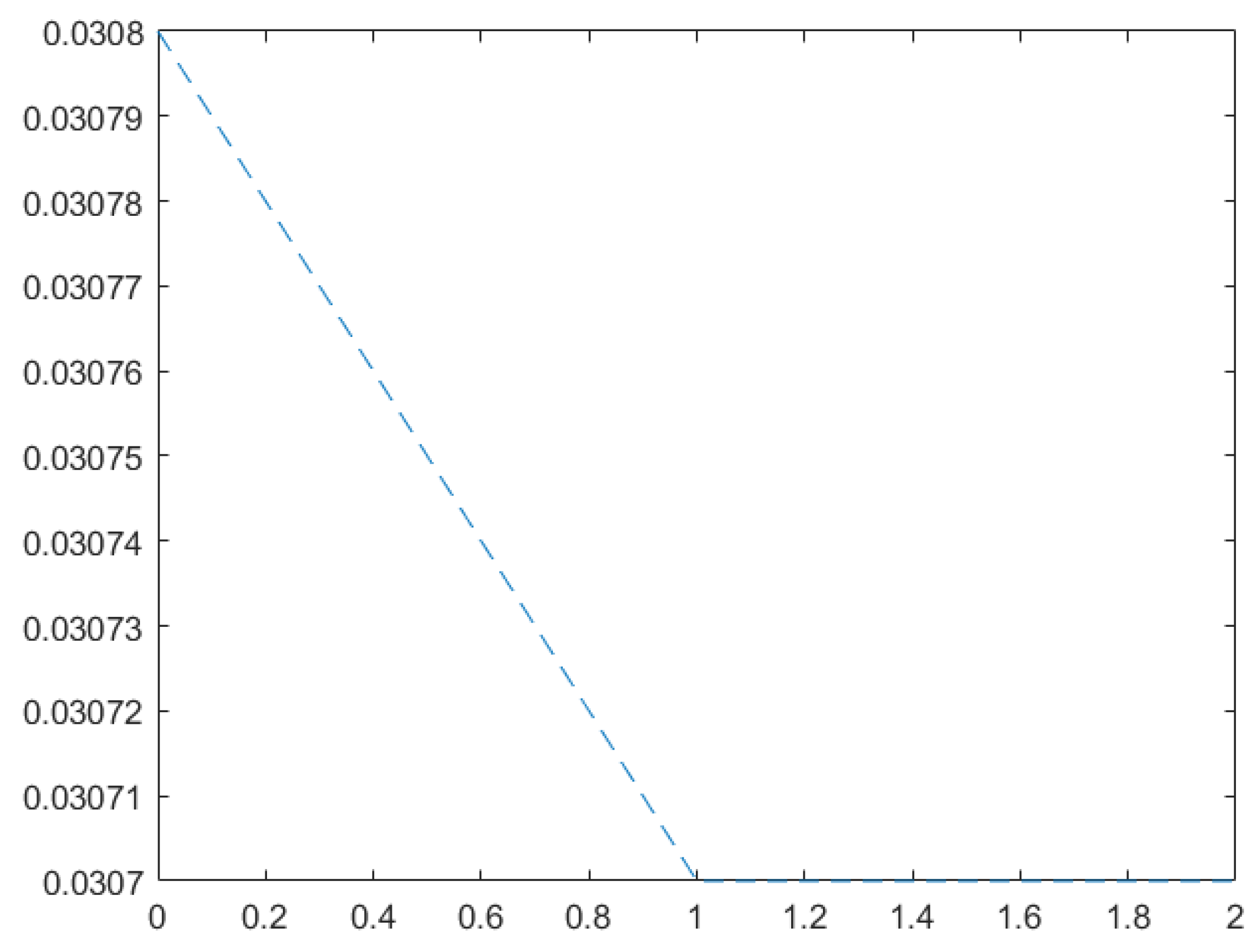
Given the conditions of Theorem 3, it is simple to demonstrate that Equation (20) has a unique solution for $\mathfrak{z}=1$ and $\varrho =1$. Additionally, we will emphasize the viability of our strategies using the iteration process.

$$\begin{array}{c}\hfill {\mu }_{\vartheta +1}\left(\nu \right)={\int }_0^1[{\left(\nu (1-\varrho )\right)}^{\varsigma -1}-{(\nu -\varrho )}^{\varsigma -1}]cos\left({\mu }_{\vartheta }\left(\varrho \right)\right)\delta \varrho .\end{array}$$

Let $\varsigma \in (1,2)$. Let us take $\varsigma =1.5$ and initial point ${\mu }_0\left(\nu \right)=0$. The sequence ${\mu }_{\vartheta +1}\left(\nu \right)={\int }_0^1[{\left(\nu (1-\varrho )\right)}^{\varsigma -1}-{(\nu -\varrho )}^{\varsigma -1}]cos\left({\mu }_{\vartheta }\left(\varrho \right)\right)\delta \varrho$ is shown in

Table 1. For $\nu =0.1$ exact solution is $\mu \left(0.1\right)=0.033$.

$\mathsf{\vartheta }$	${\mathsf{\mu }}_{\mathsf{\vartheta }+1}\left(0.1\right)$	Approximate Solution	Absolute Error
0	${\mu }_1\left(0.1\right)$	0.0308	$2.5\times {10}^{-3}$
1	${\mu }_2\left(0.1\right)$	0.0307	$2.6\times {10}^{-3}$
2	${\mu }_3\left(0.1\right)$	0.0307	$2.6\times {10}^{-3}$

for $\nu =0.1$ converge to the exact solution $\mu \left(0.1\right)=\top \left(\mu \right(0.1\left)\right)=0.033$.

We obtain the interpolated graphs of nonlinear integral equation for $\nu =0.1$, we get the following interpolated graphs, Figure 1 respectively.

Example 7.

Assume the following nonlinear integral equation.

$$\begin{array}{c}\hfill \mu \left(\nu \right)={\int }_0^1\Lambda (\nu ,\varrho )\Theta (\varrho ,\mu \left(\varrho \right))\delta \varrho ,\mathrm{for}\mathrm{all}\varrho \in [0,1]\end{array}$$

Then it has a solution in ⊤.

Proof. 

Let $\top :{\rm Y}\to {\rm Y}$ be defined by

$$\begin{array}{c}\hfill \top \mu \left(\nu \right)={\int }_0^1\Lambda (\nu ,\varrho )\Theta (\varrho ,\mu \left(\varrho \right))\delta \varrho ,\end{array}$$

and set $\Lambda (\nu ,\varrho )\Theta (\varrho ,\mu \left(\varrho \right))=\frac{3}{4}\varrho \Theta (\varrho ,\mu \left(\varrho \right))$ and $\Lambda (\nu ,\varrho )\Theta (\varrho ,\eta \left(\varrho \right))=\frac{3}{4}\varrho \Theta (\varrho ,\eta \left(\varrho \right))$, for all $\mu ,\eta \in [0,1]$. Then we have

$$\begin{array}{cc}\hfill {|\Lambda (\nu ,\varrho )\Theta (\varrho ,\mu \left(\varrho \right))+\Lambda (\nu ,\varrho )\Theta (\varrho ,\eta \left(\varrho \right))|}^2& =|\frac{3}{4}\varrho \Theta (\varrho ,\mu \left(\varrho \right))+\frac{3}{4}{\varrho \Theta (\varrho ,\eta \left(\varrho \right))|}^2\hfill \\ \hfill & =\frac{9}{16}{\varrho }^2{|\Theta (\varrho ,\mu \left(\varrho \right))+\Theta (\varrho ,\eta \left(\varrho \right))|}^2\le {\delta }_{♭}(\mu ,\eta ).\hfill \end{array}$$

Furthermore, see that $\frac{3}{4}{\int }_0^1{\varrho }^2\delta \varrho =\frac{3}{4}\left(\frac{{\left(1\right)}^3}{3}-\frac{{\left(0\right)}^3}{3}\right)=\frac{1}{4}\le 1$. Then, it is easy to see that all other conditions of the above application are easy to examine and the above problem has a solution in ⊤. □

6. Conclusions

In this manuscript, we established a orthogonal convex structural contraction mapping, proved a number of fixed point theorems utilizing orthogonal ♭-metric space, and demonstrated the existence of a solution to a unique integral equation developed in mechanical engineering.

References

1. Agarwal, R.P.; Meehan, M.; O’regan, D. Fixed Point Theory and Applications; Cambridge University Press: Cambridge, UK, 2001. [Google Scholar]
2. Alghamdi, M.A.; Hussain, N.; Salimi, P. Fixed point and coupled fixed point theorems on ♭-Metric-like spaces. J. Inequalities Appl. 2013, 2013, 1–25. [Google Scholar] [CrossRef] [Green Version]
3. Bota, M.F.; Karapinar, E. A note on “Some results on multi-valued weakly Jungck mappings in ♭-Metric space”. Open Math. 2013, 11, 1711–1712. [Google Scholar] [CrossRef]
4. Alsulami, H.H.; Karapinar, E.; Piri, H. Fixed points of generalized-Suzuki type contraction in complete-metric spaces. Discret. Dyn. Nat. Soc. 2015, 2015, 1–8. [Google Scholar] [CrossRef] [Green Version]
5. Kadelburg, Z.; Radenović, S. Notes on some recent papers concerning F-contractions in ♭-Metric spaces. Constr. Math. Anal. 2018, 1, 108–112. [Google Scholar] [CrossRef]
6. Mitrović, Z.D. A note on the results of Suzuki, Miculescu and Mihail. J. Fixed Point Theory Appl. 2019, 21, 1–4. [Google Scholar] [CrossRef]
7. Popescu, O.; Stan, G. Two fixed point theorems concerning F-contraction in complete metric spaces. Symmetry 2020, 12, 58. [Google Scholar] [CrossRef] [Green Version]
8. Saleem, N.; Iqbal, I.; Iqbal, B.; Radenović, S. Coincidence and fixed points of multivalued F-contractions in generalized metric space with application. J. Fixed Point Theory Appl. 2020, 22, 81. [Google Scholar] [CrossRef]
9. Czerwik, S. Contraction mappings in ♭-Metric spaces. Acta Math. Inform. Univ. Ostrav. 1993, 1, 5–11. [Google Scholar]
10. Debnath, P.; Konwar, N.; Radenović, S. Metric Fixed Point Theory: Applications in Science, Engineering and Behavioural Sciences; Springer: Singapore, 2021; pp. 314–316. [Google Scholar]
11. Latif, A.; Al Subaie, R.F.; Alansari, M.O. Fixed points of generalized multi-valued contractive mappings in metric type spaces. J. Nonlinear Var. Anal. 2022, 6, 123–138. [Google Scholar]
12. Jiang, S.; Wu, Y. An example of a metric space with finite decomposition complexity. J. Nonlinear Funct. Anal. 2022, 2022, 27. [Google Scholar]
13. Shatanawi, W.; Rajić, V.Ć.; Radenović, S.; Al-Rawashhdeh, A. Mizoguchi-Takahashi-type theorems in tvs-cone metric spaces. Fixed Point Theory Appl. 2012, 2012, 1–7. [Google Scholar] [CrossRef] [Green Version]
14. Takahashi, W. A convexity in metric space and nonexpansive mappings. I. Inkodai Math. Semin. Rep. 1970, 22, 142–149. [Google Scholar] [CrossRef]
15. Goebel, K.; Kirk, W.A. Iteration processes for nonexpansive mappings. J. Contemp. Math. 1983, 21, 115–123. [Google Scholar]
16. Ding, X.P. Iteration processes for nonlinear mappings in convex metric spaces. J. Math. Anal. Appl. 1988, 132, 114–122. [Google Scholar] [CrossRef]
17. Reich, S.; Shafrir, I. Nonexpansive iterations in hyperbolic spaces. Nonlinear Anal. 1990, 19, 537–558. [Google Scholar] [CrossRef]
18. Mureşan, V.; Mureşan, A.S. On the theory of fixed point theorems for convex contraction mappings. Carpathian J. Math. 2015, 31, 365–371. [Google Scholar] [CrossRef]
19. Latif, A.; Sintunavarat, W.; Ninsri, A. Approximate fixed point theorems for partial generalized convex contraction mappings in α-complete metric spaces. Taiwan. J. Math. 2015, 19, 315–333. [Google Scholar] [CrossRef]
20. Georgescu, F. Iterated function systems consisting of generalized convex contractions in the framework of complete strong ♭-Metric spaces. Ann. West Univ. Timis. Math. Comput. Sci. 2017, 55, 119–142. [Google Scholar] [CrossRef] [Green Version]
21. Karaca, N.; Yildirim, I. Fixed point theorem for Reich contraction mapping in convex ♭-Metric spaces. Aligarh Bull. Math. 2021, 40, 29–39. [Google Scholar]
22. Chen, L.; Yang, N.; Zhao, Y. Fixed point theorems for the Mann’s iteration scheme in convex graphical rectangular ♭-Metric spaces. Optimization 2021, 70, 1359–1373. [Google Scholar] [CrossRef]
23. Dolićanin-Ðekić, D.; Bin-Mohsin, B. Some new fixed point results for convex contractions in ♭-Metric spaces. Univ. Thought Publ. Nat. Sci. 2019, 9, 67–71. [Google Scholar] [CrossRef] [Green Version]
24. Asif, A.; Khan, S.U.; Abdeljawad, T.; Arshad, M.; Savas, E. 3D analysis of modified F-contractions in convex ♭-Metric spaces with application to Fredholm integral equations. AIMS Math. 2020, 5, 6929–6948. [Google Scholar] [CrossRef]
25. Berinde, V. Approximating fixed points of almost convex contractions in metric spaces. Ann. Acad. Rom. Sci. Ser. Math. Appl. 2020, 12, 11–23. [Google Scholar] [CrossRef]
26. Bisht, R.K.; Rakočević, V. Fixed points of convex and generalized convex contractions. Rend. Circ. Mat. Palermo Ser. 2020, 69, 21–28. [Google Scholar] [CrossRef]
27. Chen, L.; Li, C.; Kaczmarek, R.; Zhao, Y. Several fixed point theorems in convex ♭-Metric spaces and applications. Mathematics 2020, 8, 2422. [Google Scholar] [CrossRef]
28. Khan, M.S.; Singh, Y.M.; Maniu, G.; Postolache, M. On generalized convex contractions of type-2 in ♭-Metric and 2-metric spaces. J. Nonlinear Sci. Appl. 2017, 10, 2902–2913. [Google Scholar] [CrossRef] [Green Version]
29. Nallaselli, G.; Gnanaprakasam, A.J.; Mani, G.; Mitrović, Z.D.; Aloqaily, A.; Mlaiki, N. Integral equation via fixed point theorems on a new type of convex contraction in ♭-Metric and 2-metric spaces. Mathematics 2023, 11, 344. [Google Scholar] [CrossRef]
30. Gordji, M.E.; Ramezani, M.; De La Sen, M.; Cho, Y.J. On orthogonal sets and Banach fixed point theorem. Fixed Point Theory 2017, 18, 569–578. [Google Scholar] [CrossRef]
31. Gordji, M.E.; Habibi, H. Fixed point theory in generalized orthogonal metric space. J. Linear Topol. Algebra 2017, 6, 251–260. [Google Scholar]
32. Sawangsup, K.; Sintunavarat, W.; Cho, Y.J. Fixed point theorems for orthogonal F-contraction mappings on O-complete metric spaces. J. Fixed Point Theory Appl. 2020, 22, 1–14. [Google Scholar] [CrossRef]
33. Arul Joseph, G.; Gunasekaran, N.; Absar, U.H.; Gunaseelan, M.; Imran, A.B.; Kamsing, N. Common fixed-points technique for the existence of a solution to fractional integro-differential equations via orthogonal Branciari metric spaces. Symmetry 2022, 14, 1859. [Google Scholar]
34. Beg, I.; Mani, G.; Gnanaprakasam, A.J. Fixed point of orthogonal F-Suzuki contraction mapping on O-complete ♭-Metric spaces with applications. J. Funct. Spaces 2021, 2021, 1–12. [Google Scholar] [CrossRef]
Figure 1. Interpolated graph for t = 0.1.
Axioms 12 00143 g001