Article

Mass Generation via the Phase Transition of the Higgs Field

by
Dimitris M. Christodoulou
1,*,† and
Demosthenes Kazanas
2,*,†
1
Lowell Center for Space Science and Technology, University of Massachusetts Lowell, Lowell, MA 01854, USA
2
NASA/GSFC, Astrophysics Science Division, Code 663, Greenbelt, MD 20771, USA
*
Authors to whom correspondence should be addressed.
The authors contributed equally to this work.
Axioms 2023, 12(12), 1093; https://doi.org/10.3390/axioms12121093
Submission received: 30 October 2023 / Revised: 24 November 2023 / Accepted: 28 November 2023 / Published: 29 November 2023
(This article belongs to the Special Issue Mathematical Cosmology)

Abstract

:
The commonly quoted bistable Higgs potential is not a proper description of the Higgs field because, among other technical reasons, one of its stable states acquires a negative expectation value in vacuum. We rely on formal catastrophe theory to derive the form of the Higgs potential that admits only one positive mean value in vacuum. No symmetry is broken during the ensuing phase transition that assigns mass to the Higgs field; only gauge redundancy is “broken” by the appearance of phase in the massive state, but this redundancy is not a true symmetry of the massless field. Furthermore, a secondary, certainly amusing conclusion, is that, in its high-energy state, the field oscillates about its potential minimum between positive and negative masses, but it is doubtful that such evanescent states can survive below the critical temperature of 159.5 GeV, where the known particles were actually created.

1. Introduction

Bistable potential wells possessing two minima separated by an energy barrier are quite common in the natural sciences [1,2,3,4,5,6]. Despite their frequent use in descriptions of discontinuous transitions occurring in physical, chemical, and biological systems and their intimate connections to catastrophe theory, bifurcation theory, singularity theory, structural stability, and phase transitions [4,5,6,7,8,9], the ensuing dynamical evolution is not understood in virtually all cases, to the point that some famous accounts of transitions are not only technically unphysical, but they are also visibly preposterous. The deeper reason for such absurdities is the lack of temporal variables in Landau’s phase-transition theory and in Thom’s catastrophe theory. These theories apply only to gradient systems [1,4,5,6], and the notion of time-dependent phenomena is added ad hoc by describing arbitrarily drawn paths in the control parameter space of the cusp and higher elementary catastrophes.
For instance, Landau’s phenomenological theory of second-order phase transitions predicts the appearance of two minima of equal depth past the critical point, although we know from experiments that only one stable state exists below the critical temperature T c . To work around this problem, the theory postulates, against the odds, that an evolving system will arbitrarily choose to settle into one of these states. Even in this hypothetical scenario, the model remains unphysical because these states continue to evolve and change their mean values as the temperature T < T c is lowered toward absolute zero. So, no matter which minimum the system “chooses”, it finds itself out of equilibrium all the time; thus, the system has to evolve again and again trying to catch up with the ever-changing equilibrium state. In contemporary parlance, such a situation is described by the metaphor “moving the goalposts” which has a negative connotation.
Furthermore, it is well-known that an infinitesimal linear perturbation wipes out entirely Landau’s second-order phase transition [6], which means that such transitions should not occur in nature, or that the theory is wrong. All these absurdities come to life because of the assumption that the system finds itself at a local maximum of the potential as T crosses to just below T c , where it sees two new minima opening up as the control parameter becomes nonzero (negative, to be specific [1,5,6,7]). This assumption places the system in an unstable initial state, a practice that is heavily at odds with basic physics and with the stable stationary states that we describe in Section 2 below. It is also mathematically puzzling how the initial potential minimum at T T c changes directly to an isolated maximum without passing through a degenerate inflection point (this procedure builds a priori a discontinuity in the second derivative of the potential [1]).
The stability of the Higgs potential in particle physics [9,10,11,12,13] is another case in point. The descriptions of how the Higgs field acquires mass are cursory and nonsensical at their roots: At high energies, the massless Higgs field is supposed to be stripped of any and all features, yet it is hypothesized to have “some high symmetry” (zero weak isospin?)1 supporting an even potential function. This is the symmetry that will be broken in the final stationary state, when the unstable field will conveniently ignore the negative-minimum state and it will choose against the odds to settle into the other available state of positive vacuum expectation value (VEV). But how can such a symmetry be broken when the potential continues to be an even function, just as prior to the transition? And how can the system ever settle into either one of the low-energy states, when these states are not really stationary but continue to move the goalposts (dotted curves in Figure 1) to different VEVs all the time?
All of the above descriptions should have been taken with a large grain of salt because, after all, an infinitesimal linear perturbation at T = T c eliminates the second-order phase transition altogether. This occurs because Landau’s assumption of a “higher symmetry” in the initial state [1] arbitrarily alters the perturbation2 ( m 2 ϕ 2 / 2 + b ϕ ) attached to Thom’s cusp catastrophe germ ( ϕ 4 ; [4]); as a result, one control parameter is eliminated ( b = 0 ; [6]) and the drawn ad hoc evolutionary path { m , b = 0 } in the control parameter space ( m , b ) becomes incorrect and irreparable—even if an infinitesimal b 0 perturbation is brought back in. The reason for this structural instability is that m and b are related along the transition path; thus, the value of b cannot be chosen independently. The proof is given in Section 2.1 below using polynomial theory.
The resulting overconstrained ( b = 0 ) potential with one remaining control parameter, V ( ϕ ) = ϕ 4 m 2 ϕ 2 / 2 , is illustrated in Figure 1. The phase-transition path highlighted by the dotted curves is unphysical for the reasons discussed above; thus, naturally occurring phase transitions (of first and second order) require a different mathematical approach. We undertake this task for the Higgs field in Section 2, and we discuss our results for the various types of phase transitions in Section 3. Finally, we summarize our conclusions in Section 4. For the sake of completeness of the methodology, the two higher-order elementary catastrophes (the swallowtail and the butterfly) are also analyzed in this work, and their results are collected in Appendix A.

2. Derivation of the Higgs Potential from Catastrophe Theory

In cosmology and particle physics, the scalar Higgs field is massless and featureless at the very high energies occurring right after the big bang [9,10,14,15,16,17]. When the universe cools down to a critical temperature of T c = 159.5 ± 1.5 GeV [16,17], the electroweak phase transition takes place [9,10,11,16,17,18,19,20]. Lattice monte-carlo simulations indicate that the cross-over of the Higgs field is smooth but fast, lasting for only Δ T 5 GeV [16,17], during which the field settles down to a nonzero (positive) VEV of v = 246.22 GeV, where it has remained until the present time. This value of the Higgs VEV is a natural constant [20], and it is responsible for the corresponding particle, the Higgs boson, acquiring its observed mass (125.25 GeV; [21,22,23,24]).
There are two methods by which we can derive the scalar Higgs potential at all temperatures and observe the phase transition to the massive Higgs boson. The first derivation is more tedious and requires more steps, but it is also transparent in justifying the various assumptions being made; it further shows that the Higgs potential obeys Thom’s theorem [4] for the cusp catastrophe. The second derivation is an astute shortcut, but it is opaque and reveals no details; this formulation hides the influence of catastrophe theory, so it could have been carried out at the time that Landau [1] presented his phase-transition theory. We summarize both methods below.

2.1. Method 1: Relying on Catastrophe Theory and Stable Isolated States

For the Higgs potential V ( ϕ ) to generally exhibit three isolated extrema, its derivative V must have the form
V ( ϕ ; a , b , c ) = 4 ( ϕ + a ) ( ϕ + b ) ( ϕ + c ) ,
where a , b , c are interrelated control parameters to be constrained below. Then, V ( ϕ 0 ) = 0 gives the extrema ϕ 0 = a , b , c . Integrating Equation (1), we find that
V ( ϕ ; a , b , c ) = ϕ 4 + 4 3 a + b + c ϕ 3 + 2 a b + b c + c a ϕ 2 + 4 a b c ϕ ,
where the integration constant has been dropped. In the neighborhood of the critical point of the germ V = ϕ 4 , the Taylor expansion does not have a cubic term or terms higher than O ( ϕ 4 ) . These terms are eliminated by Thom’s inhomogeneous linear transformation and his nonlinear transformation, respectively [4,5,6]. Thus, we must set
a + b + c = 0 ,
in which case we obtain the canonical form of the cusp catastrophe3
V ( ϕ ; a , b ) = ϕ 4 2 a 2 + a b + b 2 ϕ 2 4 a b a + b ϕ ,
with the extrema located at ϕ 0 = a , b , ( a + b ) . Note that if we arbitrarily choose b = 0 , then we obtain Landau’s [1] potential with extrema at ϕ 0 = 0 , ± a (see also Section 2.2.2 below). This choice is unjustifiable, and we are not going to adopt it. Instead, we shift V ( ϕ ) by a to the right, in order to place the first listed extremum at ϕ 0 = 0 . The shift transforms the cusp-catastrophe Function (4) to
V ( ϕ ; a , b ) = ϕ 4 4 a ϕ 3 + 2 a b 2 a + b ϕ 2 ,
where an additive constant has been dropped (eliminated by a vertical shift). In this function, the extrema have been shifted to ϕ 0 = 0 , ( a b ) , ( 2 a + b ) . We shall see that ϕ 0 = 0 corresponds to a local minimum of V ( ϕ ; a , b ) , and we are prepared to assume that the massless Higgs field occupies this minimum while waiting for a more stable state to open up and become accessible. The subject of accessibility of a new global minimum is very important in this regard; it is discussed further in Section 3 below.
Next, we fix the third listed extremum to always be located at ϕ 0 = 1 by convention. Then, we set
b = 1 2 a ,
and Equation (5) takes the form
V ( ϕ ; a ) = ϕ 4 4 a ϕ 3 + 2 3 a 1 ϕ 2 .
The extrema are now located at ϕ 0 = 0 , ( 3 a 1 ) , 1 . When ϕ 0 = 1 is a global minimum, it represents the massive state of the Higgs field, and when this minimum becomes accessible at a critical point in the control parameter plane ( a , b ), the field will make the transition to a nonzero VEV ( v = ϕ 0 = 1 ). The phase-transition path is described by Equation (6). Thus, the path is an oblique line that does not cross the apex a = b = 0 of the separatrix.
In a final step, we redefine the location of the second listed extremum ϕ 0 = 3 a 1 by adopting
k 3 a 1 .
This definition gives us a better handle on the location of this extremum. We want it to correspond to a local maximum (the location of an energy barrier that obstructs the phase transition for all k ( 0 , 1 ] . As such, k should be located between the other two extrema, viz.
0 k 1 ,
and then Equation (7) is rewritten in the final form
V ( ϕ ; k ) = ϕ 4 4 3 k + 1 ϕ 3 + 2 k ϕ 2 .
Looking at this potential function, it is hard to imagine that it satisfies Thom’s cusp-catastrophe theorem [4], but it does. Equation (10) is equivalent to the cusp-catastrophe potential (4) shifted by a to the right, where a = ( k + 1 ) / 3 and b = ( 1 2 k ) / 3 .
The Higgs potential (10) is plotted across the transition path { k = 1 0 } in Figure 2. The critical points ( ϕ 0 , V ( ϕ 0 ) ) of the potential V ( ϕ ; k ) are
ϕ 0 = 0 , V ( 0 ) = 0 ; ϕ 0 = k , V ( k ) = k 3 ( 2 k ) / 3 ; ϕ 0 = 1 , V ( 1 ) = ( 2 k 1 ) / 3 .
Thus, the height of the energy barrier is Δ V = k 3 ( 2 k ) / 3 and 0 Δ V 1 / 3 . For k 1 / 2 , once at the top of the barrier, a system will dissipate an amount of energy equal to Δ E = ( 1 k ) 3 ( 1 + k ) / 3 during its settling to the global minimum on the right side. This amount is maximized at the critical point k = 0 for which Δ E max = 1 / 3 .
For k = 1 / 2 , where the two minima have equal depth, the barrier height is Δ V = 1 / 16 , and an equal amount of energy, if gained from external perturbations, will be dissipated away ( Δ E = 1 / 16 ) during the transition from the top of the barrier to one of the two stable states. The k = 1 / 2 stage is important because it is the first instance along the evolutionary path { k = 1 0 } , where another stable state ( ϕ 0 = 1 ) becomes available to a system located at ϕ 0 = 0 , although, barring a sufficiently strong nonlinear perturbation, the new state is not dynamically accessible because of the intervening barrier [28,29,30,31,32]. In Section 3, we discuss the types of viable phase transitions along the latter path segment { k = 1 / 2 0 } , where the energy barrier continues to diminish with decreasing k.

2.2. Method 2: Implementing a Shortcut

An alternative derivation of Equation (10) that dispenses with details and formalities is as follows.
We return to Equation (1) for the derivative V ( ϕ ) , which we copy here for convenience:
V ( ϕ ; a , b , c ) = 4 ( ϕ + a ) ( ϕ + b ) ( ϕ + c ) .
Following Landau’s assumption ( C ϕ 3 0 ; [1]), we eliminate the quadratic term from V , in which case the sum of the three zeros is set to zero and c = a b :
V ( ϕ ; a , b ) = 4 ( ϕ + a ) ( ϕ + b ) ( ϕ a b ) .
We shift ϕ by a to the right to place one extremum always at ϕ 0 = 0 :
V ( ϕ ; a , b ) = 4 ϕ ( ϕ a + b ) ( ϕ 2 a b ) .
We constrain the control parameters by 2 a + b = 1 (or by a b = 1 ) to place another extremum always at a fixed location ϕ 0 = 1 :
V ( ϕ ; a ) = 4 ϕ ( ϕ 1 ) ( ϕ 3 a + 1 ) .
We redefine 3 a + 1 by Equation (8) to simplify the location of the remaining extremum:
V ( ϕ ; k ) = 4 ϕ ( ϕ 1 ) ( ϕ k ) .
Integrating with respect to ϕ , we obtain the form (10) for V ( ϕ ; k ) .

2.2.1. Utilizing a Familiarity Heuristic

Perhaps surprisingly, the steps taken in the shortcut above can all be avoided by utilizing a familiarity heuristic [33].
The final result can be written down in just two steps, without proof or investigation of its validity, by simply recalling that we are interested in static potentials which we can use to demonstrate phase transitions. Such potentials must generally exhibit three extrema, two fixed minima ( ϕ 0 = 0 , 1 ) representing the initial and final stationary states, and a maximum representing an obstacle or barrier that separates the two states. Therefore, Equation (16) can be written down ab initio, and then it can be integrated to yield the potential V ( ϕ ; k ) shown in Equation (10).
The problem with this extremely fast, albeit heuristic approach is, of course, that we cannot then formally justify the potential obtained by intuition and familiarity with nature’s phase transitions [1,2,3]. This problem is solved by the lengthy derivation given in Section 2.1 above.

2.2.2. Looking Back to Landau’s Theory of Phase Transitions

By contrast, Landau’s phase-transition theory can be formulated in the same context (Equations (12)–(16)) as follows.
Control parameter c is replaced by ( a + b ) in Equation (12) to eliminate the ϕ 2 term (no cubic term in the potential). Then, b is set to zero in Equation (13) (in disagreement with catastrophe theory, which was not known at that time), resulting in the overconstrained form
V ( ϕ ; a ) = 4 ϕ ( ϕ 2 a 2 ) .
Integrating with respect to ϕ , we obtain the final form
V ( ϕ ; a ) = ϕ 4 2 a 2 ϕ 2 ,
which is depicted in Figure 1 for a = 0 , 0.5 , 1 (corresponding to m = 0 , 1 , 2 ; here, a = m / 2 ). As was discussed in Section 1 and summarized in the caption of Figure 1, these potential curves do not form an evolutionary path in the control parameter plane ( a , b ) with varying values of the remaining control parameter { | a | = 0 0.5 1 } .

3. Discussion of Phase Transitions

3.1. The Higgs Phase Transition

For the purposes of our discussion, we rewrite the canonical potential Function (4) of the Higgs field in Thom’s equivalent form of a cusp catastrophe, viz.
V ( ϕ ) = ϕ 4 + A ϕ 2 + B ϕ ,
where the control parameters ( A , B ) are functions of two of the roots ( a , b ) of V ( ϕ ) = 0 , viz. A 2 ( a 2 + a b + b 2 ) and B 4 a b ( a + b ) . The third root c is not independent, i.e., c = ( a + b ) (Equation (3)). If we set any one of these three roots to zero, then B = 0 and the perturbation of the germ ϕ 4 takes a specialized even form that cannot describe quantitatively any phase transition since the phenomenon occurs naturally for general perturbations of no particular symmetry. Moreover, B = 0 fixes the maximum of the bistable potential V ( ϕ ) to point ( 0 , 0 ) , where the system finds itself at the onset of the phase transition. Thus, the system is unstable and has no choice but to evolve. This setup is clearly problematic.4 Physical reasoning [2,3,4,7,8,9,15,16,17,26,27,28,29,30,31,32] formally requires that the system be located at a stable minimum of the potential at all times before the second-order critical point T c is reached, and that this minimum become degenerate for T = T c (i.e., an inflection point) and progressively a (no longer relevant) local maximum for T < T c , as in Figure 2 (the case T < T c corresponds to the k = 0.25 curve). This figure also shows the physical reason for the occurrence of the second-order phase transition for k = 0 : the energy barrier that separates the two stable states diminishes as T T c + ( k 0 + ) and disappears altogether for T = T c ; in fact, it is the merging of this maximum with the minimum at ϕ 0 = 0 that makes the critical point T = T c degenerate. This smooth process makes sense, as the minimum that initially hosts the system switches gradually, first to an inflection point, and then to a maximum.
The control parameters A and B do not vary independently along the evolutionary path. Therefore, setting B = 0 for all values of A in Equation (19) (as in Landau’s theory) is prohibited. This can be proven as follows: Using Equations (6) and (8), we express the control parameters ( A , B ) of the canonical cusp catastrophe (19) as functions of k, viz.
A = 2 3 k 2 k + 1 ,
and
B = 4 27 2 k 1 k + 1 k 2 ;
we can see that B = 0 in k [ 0 , 1 ] only for a single point, k = 1 / 2 , for which A = 1 / 2 .5 Now, eliminating k between these two equations, we find that the control parameters ( A , B ) are related along the path { k = 1 0 } by
4 ( A + 2 ) 2 ( 2 A + 1 ) + 27 B 2 = 0 ,
where A [ 2 / 3 , 1 / 2 ] and B [ 8 / 27 , 8 / 27 ] . This curve effectively constrains the evolutionary path in the ( A , B ) plane; the constraint reveals the presence of an integral of motion (i.e., a conserved quantity) during the evolution, as was determined in astrophysical first-order and second-order phase transitions [29,30,31,32].
Figure 3 shows the ( A , B ) plane of the cusp potential (19) and the evolutionary path { k = 1 0 } that lies entirely within the separatrix (the fold curve 8 A 3 + 27 B 2 = 0 ) and terminates at the critical point k = 0 , where the phase transition occurs spontaneously. (Note the degenerate inflection point at ϕ 0 = 0 in the inset of the Higgs potential V ( ϕ ; 0 ) .) For k = 0 , the coordinates are ( A , B ) = ( 2 / 3 , 8 / 27 ) . Because this point also lies on the separatrix, this is the first demonstration of the so-called “delay convention” [3,4,5,6,37] in a second-order phase transition. Except that the delay down to k = 0 does not occur by convention here, it is a calculated outcome in the evolution of V ( ϕ ; k ) depicted in Figure 2. This brings the discussion to the other convention6 commonly used in catastrophe theory, the so-called “Maxwell convention” [3,6,28,37] used in first-order phase transitions.

3.2. The Maxwell Convention and Chemical Reactions

The Maxwell convention singles out the point with k = 1 / 2 in the middle of the path shown in Figure 3 as a viable phase-transition point because the two minima seen in the V ( ϕ ; 0.5 ) inset have the same depth [37,38]. This is utter speculation that came about because a system was thought to already be at the top of the energy barrier. From the top, both minima are accessible with equal probabilities of transition, and the two stable states coexist. This setup and assumptions are basically the same as in the Higgs field which can also transition to the two stable states (one with negative VEV) with equal probability, according to Landau’s theory [1]. But, as we explained above, placing a system at a local maximum at the transition point is unphysical; so, we proceed to describe and clarify the evolution of nonspontaneous first-order phase transitions and Maxwell’s rule under the action of external perturbations in the control parameter plane of Figure 3.
Maxwell’s rule [38] (the basis for the Maxwell convention) identifies the point ( k = 1 / 2 ) along the path { k = 1 0 } in Figure 3, in which the two stable minima attain equal depths. The system initially occupies the left minimum and, as the evolution proceeds along the segment { k = 1 / 2 0 } , it cannot generally access the other stable state because of the intervening energy barrier. Thus, Maxwell’s rule simply captures the first instance that another stable state becomes available, but not necessarily accessible. Only external perturbations can induce such a nonspontaneous transition of system parts and sectors for k 1 / 2 , if they are sufficiently strong, and then the two phases will coexist. Thus, chances are that such a discontinuous transition of sectors may occur at a value smaller than k = 1 / 2 because the barrier height decreases along the segment k < 1 / 2 (Figure 2).
This is precisely what takes place in the chemical reactions that use catalysts [39,40,41,42,43]; catalysts lower the so-called activation energy barrier, thereby increasing the reaction rates (i.e., they induce a first-order phase transition in parts of the reactants), without actually being consumed. Lowering the energy barrier is a mechanism used in catalyzed chemical reactions. An alternative mechanism is to perturb the reactants by supplying excess heat. In this pathway, the barrier remains intact, but the reactants absorb the energy, and more constituents go over the top of the barrier to the other state that hosts the products of the reaction.

3.3. Overcoming the Energy Barrier

The above chemical reaction mechanisms fit rigorously into our framework of first- and second-order phase transitions (Figure 2 and Figure 3). A spontaneous reaction occurs when there is no barrier ( k = 0 ); and a catalyzed reaction or a heat-driven barrier jump occurs for k 1 / 2 , but only under the action of perturbations supplying the necessary energy. An example is shown in Figure 4 for k = 0.4 in Equation (10). We consider a system oscillating initially about minimum I under the action of external perturbations. Since k < 1 / 2 , the second minimum S that became available for k = 1 / 2 is now the global minimum and the energy barrier Δ V has decreased in height past the Maxwell point.
We distinguish three cases in the free-energy diagram sketched in Figure 4:
(a)
If the Gibbs free energy Δ E gained by the parts of the system is not sufficient to push any part up to at least point P (or B), then the perturbed system remains in the neighborhood of point I.
(b)
If, on the other hand, Δ E = Δ V in some parts, then these parts displaced to point P can overcome barrier B and roll over to the new global stable state S [2,3,28,29,30,31,32]. Then, the two phases, I and S, coexist [34,35,36].
(c)
Furthermore, if Δ E > Δ V in some perturbed parts (displaced, e.g., up to point J), then these parts no longer recognize barrier B and collapse to the deep minimum S on a dynamical time [3,44,45].
In most physical systems undergoing phase transitions, the evolutionary paths just outlined cannot be obtained analytically as functions of time because the partial differential equations of motion cannot be solved analytically [46,47]. For this reason, researchers in the past have approached the subject either by studying only the stationary minima of the potentials (e.g., [28,29,30,31]), thereafter assuming that quasistatic evolution takes place between the stable states; or by relating the stationary states to analytic non-dissipative solitary-wave solutions conserving localized finite energy (the topological method of “orbits”; [47,48,49]); or by numerical simulations (e.g., [2,16,17,46]).

3.4. Star-Forming Phase Transitions

Although the outcome of the above evolutionary scenarios is the same in Figure 4 (the settling of at least parts of a system into stable state S), the dynamics is quite different. The difference was recognized long ago in the context of star formation in giant molecular clouds, first by Whitworth [28] and subsequently by Tohline [2,3,29,30,31], although the same ideas had been previously explored in various related contexts [50,51,52]. Whitworth [28] described a perturbed diffuse molecular cloud region bound by external pressure, that reaches over time [3] (point P in Figure 4, as “preunstable,” a condition that differentiates it from a region strongly compressed and displaced to point J, where it becomes Jeans unstable [44] and subject to dynamical collapse down to the compact (high-density) stellar state (point S in Figure 4). Tohline [30] recognized that the path (PIBS in Figure 4) highlights a slower phase transition (distinct from dynamical Jeans collapse) capable of producing stars of much lower masses (albeit over much longer timescales [3]), as compared to the famous Jeans critical mass [44], the hallmark of dynamical star formation since 1902 and for years to come [53].

3.5. Peculiar λ -Transitions

To complete the discussion of the various types of phase transitions encountered in nature, we should mention that some phase transitions do not fit into the modern classification scheme [35,36]. Most puzzling among them are the so-called λ -transitions [8,32,34,35,36,54,55] that may or may not [8,35] have infinite specific heat at the critical point (e.g., at the λ -point T c = 2.18 K of the superfluid liquid 4 He [34,35,36] or at the order–disorder critical point T c = 739 K of the β -brass Cu-Zn alloy [34,56]). Bose–Einstein condensation of an ideal Bose gas [34] and astrophysical binary fission and ring formation [32] are also types of λ -transitions, and the various types are all linked together only by spontaneous breaking of the topology [8,32] (the symmetry may break or not, and the specific heat may diverge or not [8,35,54,55,56]).
From the viewpoint of the energetics of discontinuous λ -transitions, we know that a total of five extrema (not all of them isolated) are involved in the Gibbs free-energy function [32], which places these transitions along paths in the higher-order butterfly catastrophe [55], if the free energy is a continuous function of the order parameter [32]. The main characteristic of the underlying potential function is an energy barrier that progressively becomes taller as T T c + , and then, it suddenly disappears just past the critical point T = T c (see, e.g., Figures 3–5 in Ref. [32]). This astonishing behavior of the free-energy barrier in astrophysical systems exhibiting topology-breaking phase transitions [57,58,59,60,61,62,63] remains under investigation to this day (see Refs. [2,3,8,29,30,31,32] for more details).

4. Conclusions

(a)
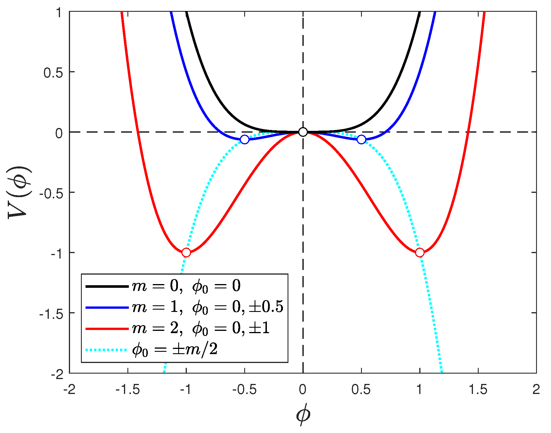
Figure 1 shows the potential functions for Landau’s phenomenological theory of second-order phase transitions [1], including that ascribed to the Higgs field. As the control parameter is increased (to simulate time evolution), the potential develops two features that render it unphysical: two symmetric stable global minima appear on either side of the local maximum at ϕ = 0 , and they both continue to move away from ϕ = 0 in time.
Thus, assuming an initial state at ϕ = 0 , as usual [4,5,6], the phase transition does not produce a unique or a universal final state. But these properties are required for the Higgs field at present [9,10,11,12,13,20]; and uniqueness of the final state is required for many phase transitions in solids and fluids [8,29,30,31,32,34,35,36,45,54].
(b)
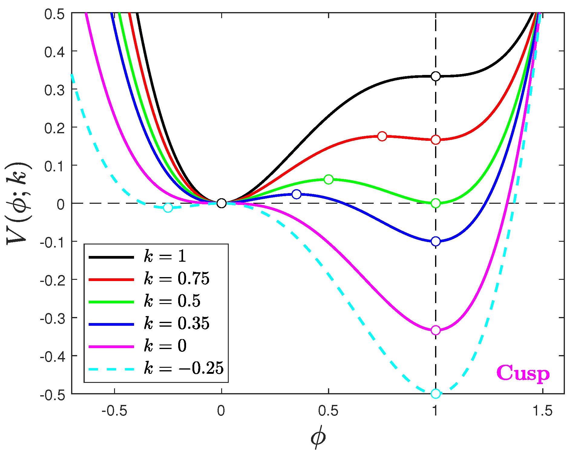
Figure 2 shows how to get around the problems highlighted above. The potential functions of the cusp catastrophe [4] are all shifted so that one minimum is always at ϕ = 0 (representing the initial state) and another minimum is constrained to always be at ϕ = 1 , making this (final) state universal [20]. The linear term of the cusp catastrophe (Equation (4)) precludes the appearance of another minimum at ϕ < 0 before the second-order critical point at k = 0 is reached; and when such a minimum finally appears for k < 0 , it is incapable of influencing the dynamics of the phase transition that took place spontaneously already for k = 0 .
The maximum that appears for 0 < k < 1 represents a free-energy barrier between the two isolated stable states. External perturbations may drive a system from ϕ = 0 to ϕ = 1 , if they supply the requisite energy to overcome the intervening barrier (a first-order phase transition [2,3,30,31]), otherwise the system remains oscillating about ϕ = 0 . As the control parameter decreases toward k = 0 (Figure 2), the barrier becomes shorter (just as in catalyzed chemical reactions [39,40,41,42,43]), and a second-order phase transition appears at k = 0 , where the barrier disappears [29,32,45]. We believe that such a transition occurred in the massless Higgs field when it acquired its uniquely positive universal VEV [16,17,20] because we cannot imagine vacuum perturbations strong enough to overcome the energy barrier in the interval 0 < k 1 / 2 .
Before the phase transition occurs, the Higgs field is induced to executing small amplitude oscillations about the minimum at ϕ = 0 that represents the equilibrium VEV of the massless state. Such oscillations generate evanescent particles with both positive and negative masses that do not survive long into the future. The observed particles of our times were all assigned masses after the Higgs field had settled to its universal VEV of 246.22 GeV [20,64].
(c)
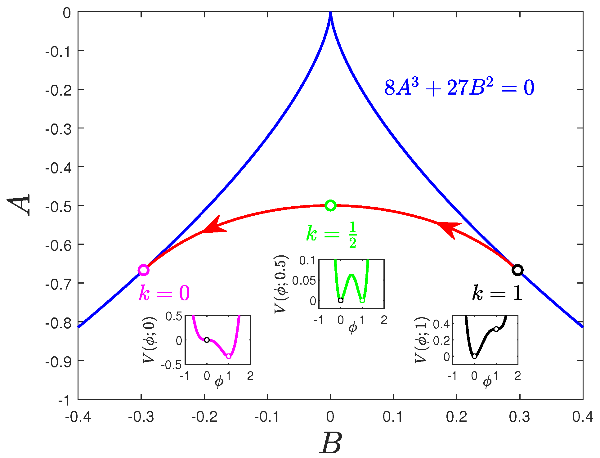
Figure 3 shows the evolutionary path in the control plane of the cusp catastrophe. The path remains within the fold lines of the separatrix at all times (even for 0 > k > 1 ), and exhibits a Maxwell critical point [37,38] for k = 1 / 2 and a second-order critical point for k = 0 .
As the green curve in Figure 2 shows, a first-order stable minimum at ϕ = 1 becomes available for k = 1 / 2 , but it is not necessarily accessible to a system located at ϕ = 0 via a first-order phase transition due to the intervening energy barrier. For the Higgs field, such a continuous line of first-order phase transitions was observed in the past (before the discovery of the Higgs boson and the measurement of its mass; see Refs. [16,17,46] and references therein); although the lattice simulations were using Landau’s even-symmetric potential and a Higgs mass of no more than 73.3 ± 6.4 GeV. For higher Higgs masses in non-perturbative simulations, the second-order critical point was replaced by a smooth crossover to the final massive state [16,17,46]. These doubtful results must have their origin in the unphysical potential used, and new simulations are needed to revisit the true nature of the Higgs phase transition.
(d)
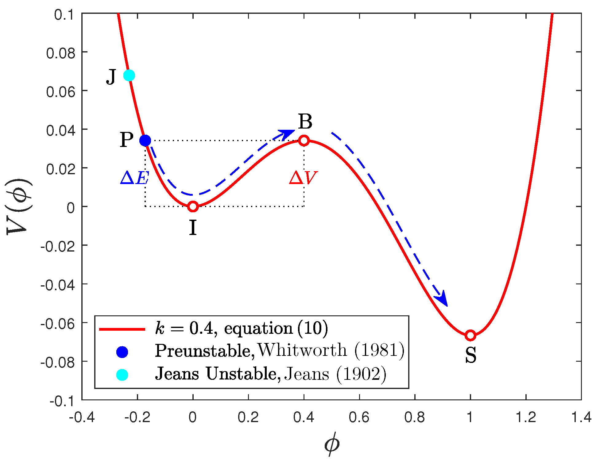
Figure 4 shows a schematic illustration of the various aspects of first-order phase transitions capable of overcoming the intervening energy barrier [3]. Basically, there are two separate evolutionary modes depending on the amount of energy deposited by acting external perturbations over time: (i) a strongly perturbed system (point J in Figure 4) is not impeded by the barrier any longer and makes the transition to the final equilibrium state S on a dynamical time [30,31,44]; and (ii) a system oscillating about point I, and perturbed gradually upward to point P (or B), gains enough energy to jump over the top of the barrier B and down to the final equilibrium state S [28,29,30].

Author Contributions

All authors have worked on all aspects of the problems, and all authors have read and agreed to the published version of the manuscript.

Funding

NASA and NSF support over the years is gratefully acknowledged. DMC acknowledges current support from NSF-AAG grant No. AST-2109004.

Data Availability Statement

No new data were generated in the course of this study.

Acknowledgments

We thank the reviewers for comments and suggestions that helped us improve the presentation of the material.

Conflicts of Interest

The authors declare no conflict of interest.

Appendix A. The Potentials of Higher-Order Catastrophes

We have carried out the derivation described in Section 2.2 for the swallowtail and butterfly catastrophes as well. To dissociate these types of potentials from the Higgs field, we use here x for the order parameter instead of ϕ . The resulting potential functions and some of their phase-transition properties are summarized below.

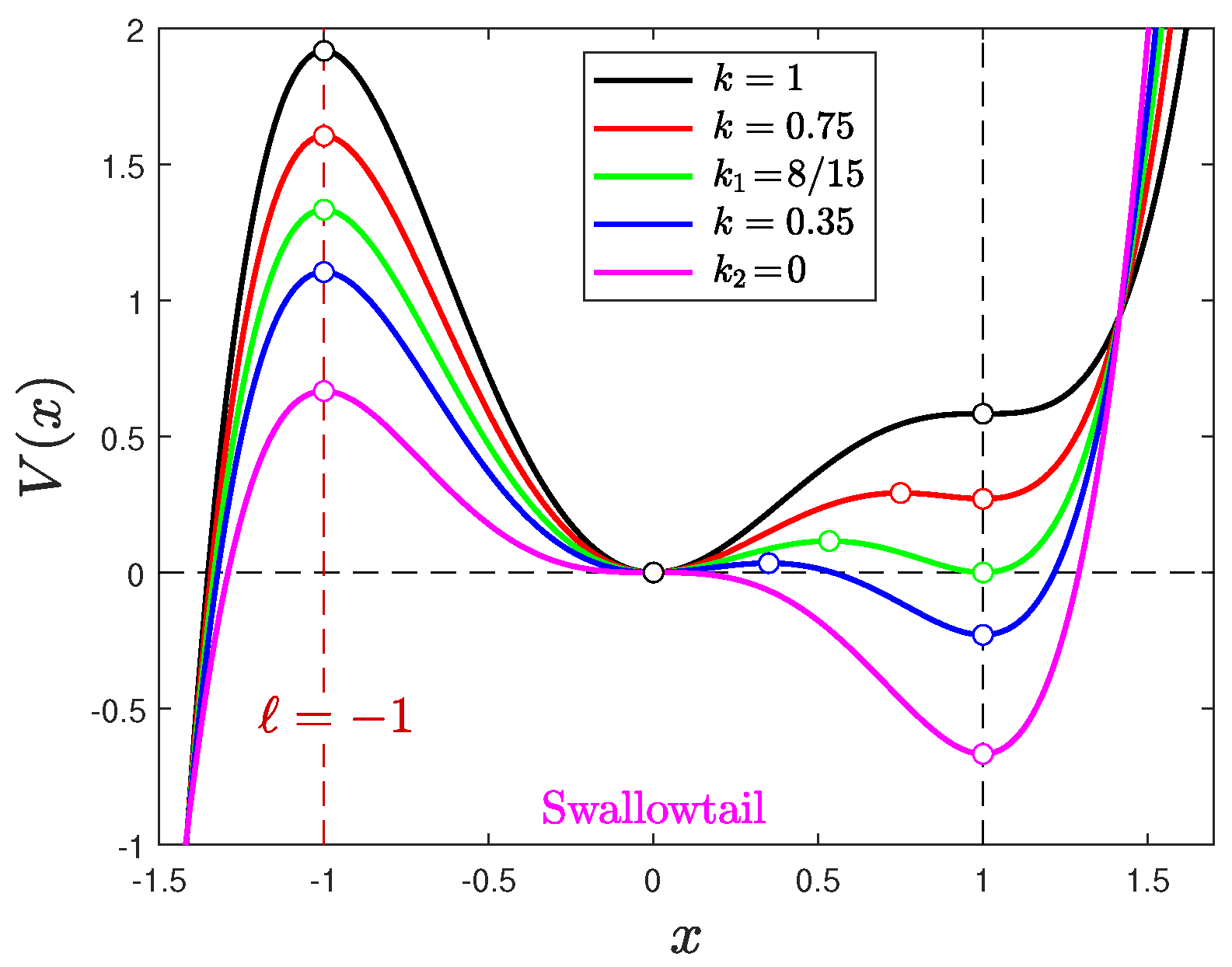
Appendix A.1. Swallowtail Potentials

The swallowtail catastrophe V ( x ) has the germ x 5 and a perturbation of O ( x 3 ) . The x 4 term is missing, so the sum of the zeroes of the derivative V ( x ) is zero. Then, one of the zeroes a , b , c , d becomes d = a + b + c and V ( x ) takes the form
V = 5 ( x + a ) ( x + b ) ( x + c ) ( x a b c ) .
Shifting V by a to the right and setting one of its zeroes to x 0 = 1 (i.e., 2 a + b + c = 1 ), we find that
V = 5 x ( x 1 ) ( x k ) ( x ) ,
where k a b and 3 a + b 1 . Integrating Equation (A2) with respect to x, we find the potential function
V ( x ) = x 5 5 4 ( k + + 1 ) x 4 + 5 3 ( k + k + ) x 3 5 2 ( k ) x 2 .
We see now that the choice of x 0 = 1 has limited the control space to only two independent parameters ( k , ). This choice, which has been overlooked for generations, is necessary to create and define another stable state, so that we can apply this potential to actual physical systems. (The initial stable state created by the shift is also fixed at x 0 = 0 .) We must say at this point that any arbitrary paths drawn in the deceiving general three-dimensional swallowtail control space are meaningless, in the sense that physical systems do not evolve unconstrained along such paths that keep moving the goalposts (see Section 1).
We also choose the extremum x 0 = k to be between 0 and 1, that is, to serve as an energy barrier between the two stable states. Thus, 0 k 1 , allowing for N = 3 possible k locations in the interval k [ 0 , 1 ] (0, 1, and in-between). Now, can be located anywhere on the x-axis, so there are N = 17 possible locations for the pair ( k , ). Of those, the extrema x 0 = 0 , 1 are local minima in only one case, in which < 0 ( N = 3 cases, if we also count the degeneracies k = 0 , 1 ). Therefore, only the case < 0 is of interest to phase transitions along the path { k = 1 0 } . Now, the isolated extremum x 0 = < 0 is always a local maximum, and it can vary just as k varies within its own interval. But variation in does not change the qualitative properties of the transition, so we can assume here for demonstration purposes that is a negative constant along the considered transition path. In a physical system, however, the variation in will have to be determined from the physical parameters of the system itself.
Phase transitions.—An illustration with constant = 1 (fixed) is shown in Figure A1. The transition proceeds on the right half of this diagram just as it does for the cusp potential in the main text. The second-order critical point appears for k 2 = 0 (the inflection point at x 0 = 0 on the magenta curve). The first-order critical point appears for k 1 = 8 / 15 (two equal-depth minima on the green curve), as determined from the equation
k 1 = 5 3 10 5 ,
for = 1 (note that k 1 1 / 2 as ± , and the cusp catastrophe is fully recovered).
Figure A1. Swallowtail potential functions for the phase-transition path { k = 1 0 } . Parameter k controls the location of the right barrier which disappears for k 2 = 0 . Parameter controls the left barrier, which we have fixed at x 0 = 1 for simplicity. The left barrier becomes shorter as 0 . A system that somehow is induced to overcome this barrier before it manages to settle to the x 0 = 1 minimum will fall apart.
Axioms 12 01093 g0a1
Left energy barrier.—Point = 1 marks the location of another energy barrier on the left side of the diagram, and this barrier may be important in some applications concerned with systems falling apart: Assuming that a system (initially executing small-amplitude oscillations about x 0 = 0 ) can somehow be induced to climb over the top of this barrier (before it settles to the stable minimum x 0 = 1 ), then this system is doomed; it will certainly be destroyed since there is no other minimum of the potential available in the region x < . This path is however of no interest in customary applications of the swallowtail catastrophe, in which researchers are studying phase transitions terminating at stable states [4,5,6,7,65,66,67,68], such as x 0 = 1 in Figure A1.

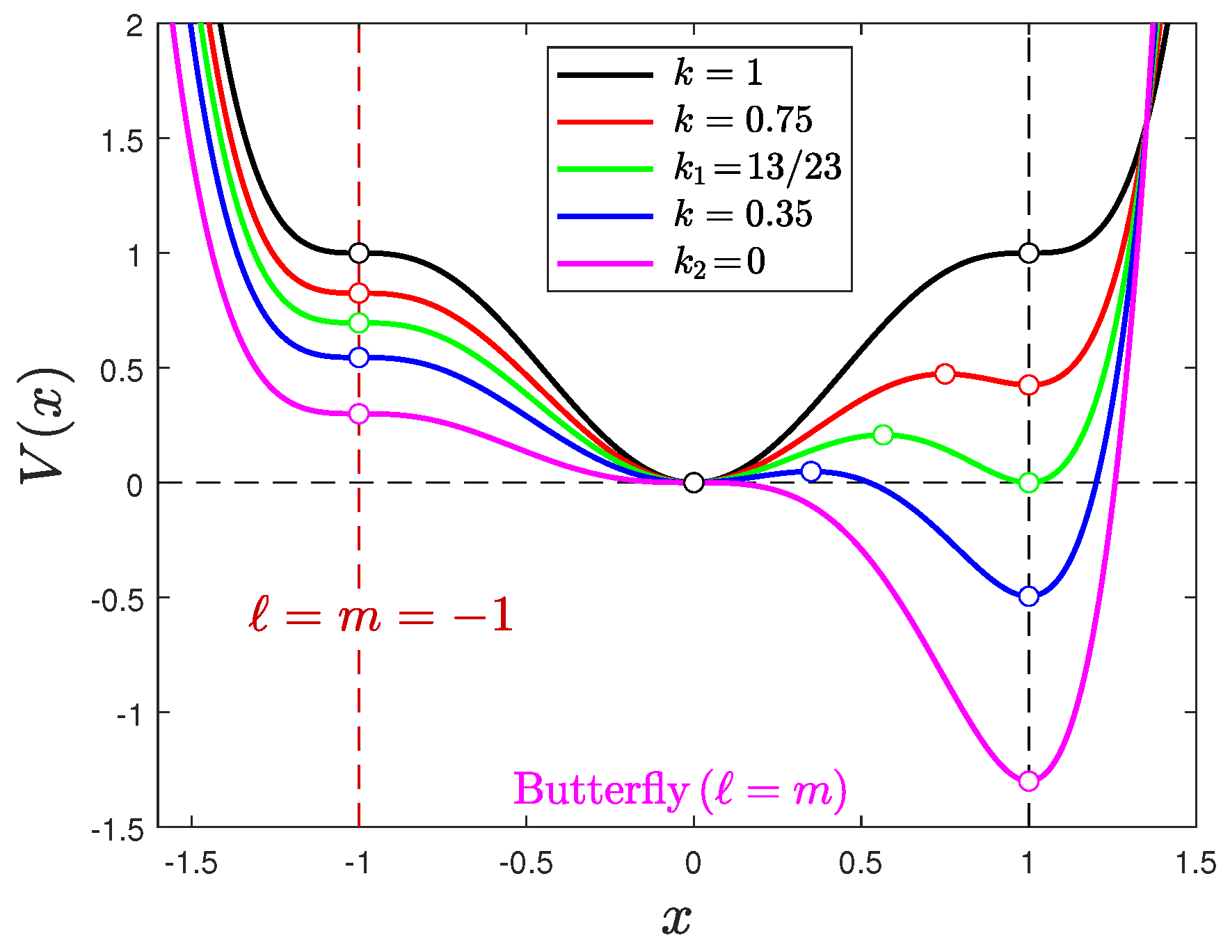
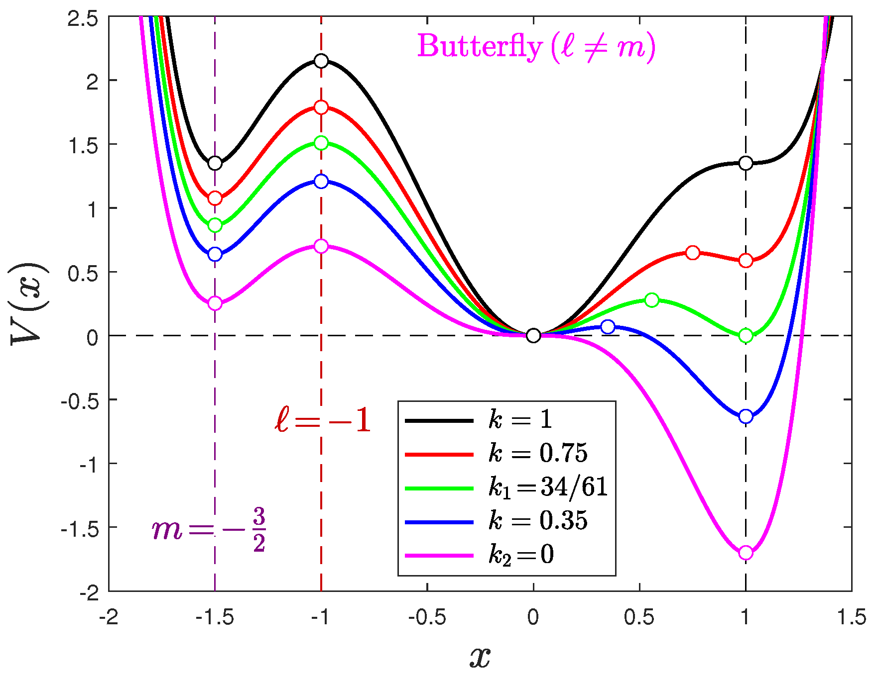
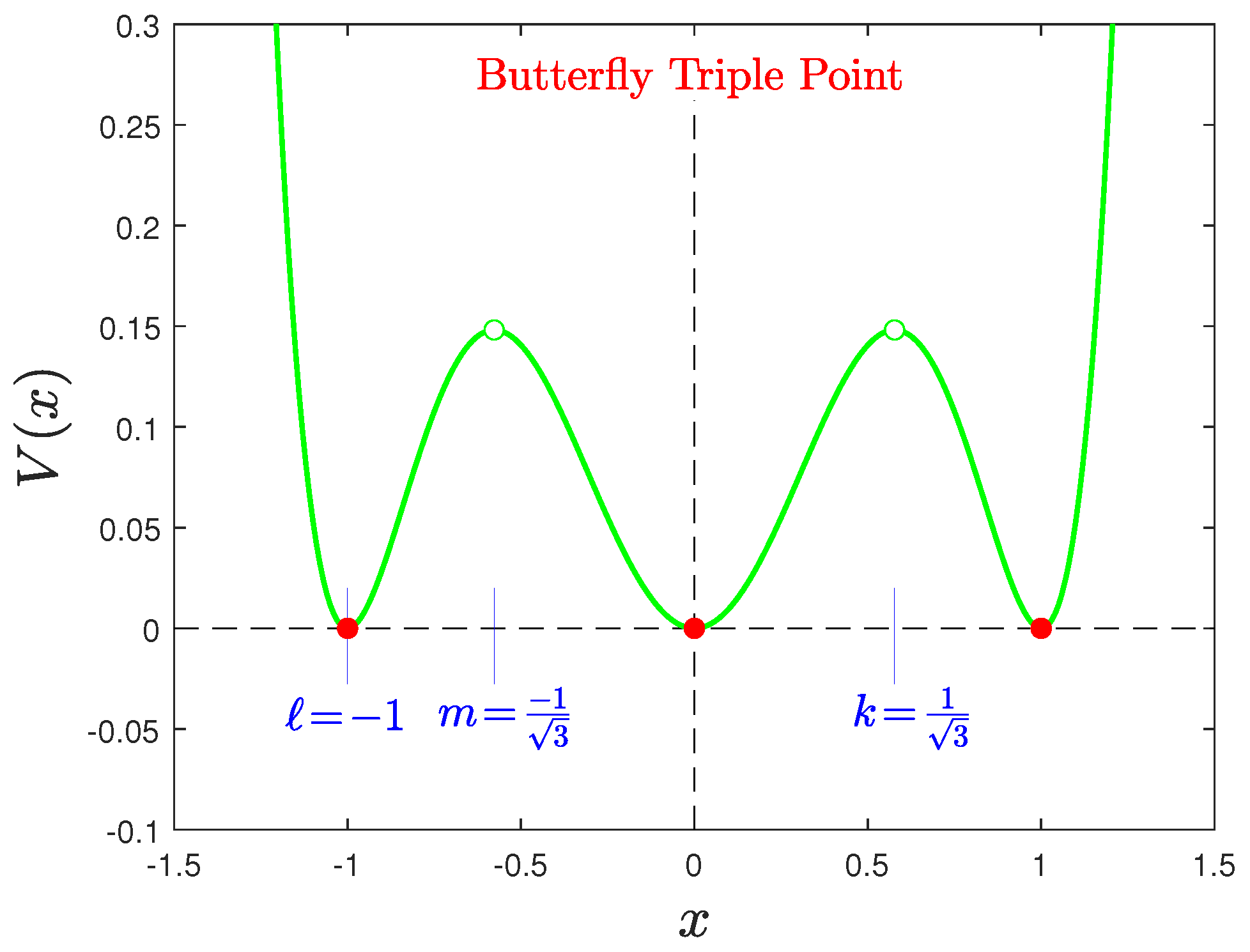
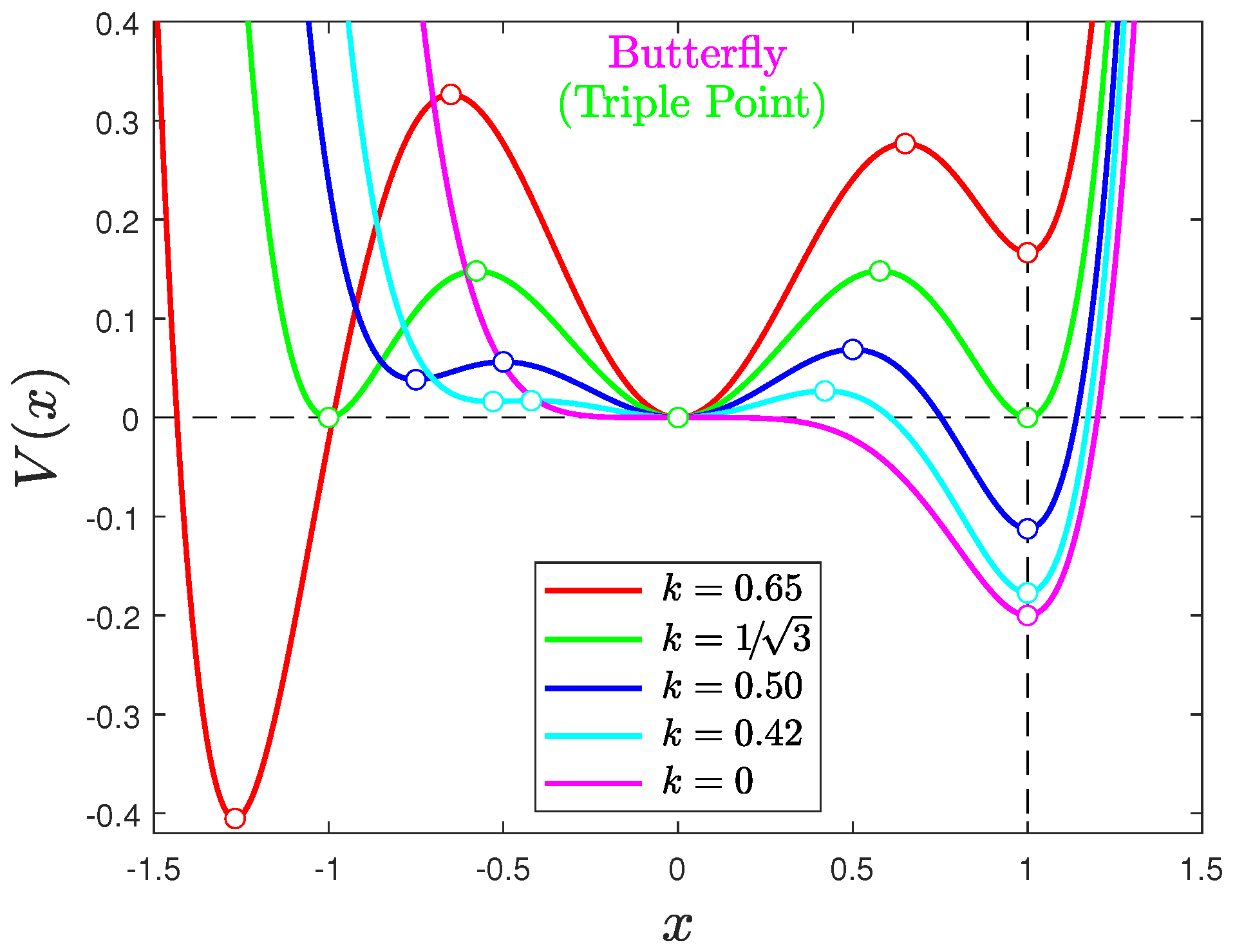
Appendix A.2. Butterfly and Triple-Point Potentials

The butterfly catastrophe V ( x ) has the germ x 6 and a perturbation of O ( x 4 ) . The x 5 term is missing, so the sum of the zeroes of the derivative V ( x ) is zero. Then, one of the zeroes a , b , c , d , e becomes e = a + b + c + d and V ( x ) takes the form
V = 6 ( x + a ) ( x + b ) ( x + c ) ( x + d ) ( x a b c d ) .
Shifting V by a to the right and setting one of its zeroes to x 0 = 1 (i.e., 2 a + b + c + d = 1 ), we find that
V = 6 x ( x 1 ) ( x k ) ( x ) ( x m ) ,
where k a b , = a c , and m 3 a + b + c 1 . Integrating Equation (A6) with respect to x, we find the potential function
V ( x ) = x 6 6 5 ( k + + m + 1 ) x 5 + 3 2 ( k ( + m + 1 ) + m + + m x 4 2 ( k ( m + + m ) + m x 3 + 3 ( k m ) x 2 .
We see now that the choice of x 0 = 1 has limited the control space to only three independent parameters ( k , , m ). Once again, this choice, which has been overlooked for generations, is necessary to create and define the second stable state, so that we can apply this potential to actual physical systems. (The initial stable state created by the shift is also fixed at x 0 = 0 ). We reiterate that arbitrary paths drawn in the deceiving general four-dimensional swallowtail space are meaningless because physical systems do not evolve unconstrained along such paths that keep moving the goalposts (see Section 1).
We choose again k [ 0 , 1 ] to provide an energy barrier between the minima x 0 = 0 , 1 . Based on the analysis in Appendix A.1, we also limit this investigation to < 0 .7 Then, there are N = 23 possible locations of the new extremum m, of which only N = 3 are worthy of further consideration (because x 0 = 0 , 1 are local minima), all of them having m < 0 . Now, Equation (A7) shows that and m are interchangeable parameters. If we choose = m , then the two extrema merge into a degenerate inflection point (at x < 0 ) of no particular interest. But if m , then another barrier appears at x 0 = max ( , m ) and a new local minimum opens up at x 0 = min ( , m ) . These two cases are illustrated in Figure A2 and Figure A3, respectively, where the locations of , m < 0 were fixed without loss of generality. We note that the left barrier at x 0 = < 0 in Figure A3 becomes shorter as 0 .
Phase transitions.—In Figure A2 and Figure A3, the phase transitions proceed on the right halves of these diagrams, just as they do for the cusp potential in the main text. The second-order critical point appears for k 2 = 0 in both figures. The first-order critical points appear for k = k 1 , as determined from the equation
k 1 = 5 m 3 ( + m ) + 2 10 m 5 ( + m ) + 3 .
Triple point.—In the diagram of Figure A3, the two minima do not have the same depth for any value of k [ 0 , 1 ] because of the arbitrary choices for and m. So, there is no triple point along this phase-transition path. Then, it is easy to recognize that the control parameters ( k , , m ) must be related for a triple point to appear in the potential (A7). Their relationships are expressed by the conditions that
V ( ) = V ( 1 ) 0 .
Here, and m are interchangeable parameters, so we chose the third minimum to be located at x 0 = . The V 0 equal-depth conditions (A9) then require that
= 1 and m = k = 1 / 3 ,
where now k and m are interchangeable (but we break the symmetry by choosing 0 k 1 , as usual). It is easy to prove then that V ( x ) at the triple point is an even function of x, and this is why the third minimum ( x 0 = or m) must be located at x 0 = 1 . In fact, the potential V ( x ) at the triple point takes the simple form
V ( x ) = x 6 2 x 4 + x 2 = x 2 ( x 2 1 ) 2 .
Figure A2. Butterfly potential functions for the phase-transition path { k = 1 0 } with = m = 1 . Parameter k controls the location of the barrier, which disappears for k 2 = 0 . Parameters , m < 0 control extrema that develop in the x < 0 region. In the = m case shown here, the extrema degenerate to an inflection point at x 0 = 1 . The height of this inflection point decreases as = m 0 .
Axioms 12 01093 g0a2
Figure A3. As in Figure A2, but for butterfly potentials with m and a second barrier at x < 0 which we have fixed at = 1 for simplicity. The two extrema in the region x < 0 are now isolated, and a new local minimum opens up at x 0 = m = 3 / 2 (again, fixed for simplicity). The height of the left barrier decreases as 0 .
Axioms 12 01093 g0a3
This reduced butterfly potential that exhibits a triple point (i.e., three minima of equal depth) is illustrated in Figure A4, where we chose k > 0 and = 1 . The choice m = 1 is of course an alternative, and then the labels and m switch places in Figure A4. With the equal-depth minima set at x 0 = 0 , ± 1 , then the extrema x 0 = k , m represent energy barriers of equal height.
Figure A4. Triple point of a butterfly potential with m . The potential is now an even function (Equation (A11)) with no independent control parameter (Equation (A10)). With x 0 = k chosen to lie in (0, 1) to provide a barrier, then interchangeable parameters , m < 0 provide the locations of the two isolated extrema on the left side (i.e., x 0 = and x 0 = m ).
Axioms 12 01093 g0a4
Finally, for an evolutionary path { k = 1 0 } that exhibits a triple point, the following general relations hold along the path:
= 3 k m and m = k ;
so, only one of the control parameters ( k , , m ) of the butterfly turns out to be independent in this model. The triple point occurs for = 1 along this path which, in terms of , is described by { = 3 0 } and terminates at the second-order critical point = 0 . Figure A5 provides an illustration of this phase transition. The control parameters of the potential Function (A7) have been reduced to functions of k by using the relations (A12), viz. = 3 k 2 and m = k , and then k is the only independent parameter along the evolutionary path.
Figure A5. As in Figure A3, but for an evolutionary path { k = 1 0 } (equivalently, { = 3 0 } ) in the butterfly catastrophe that exhibits a triple point for = 1 and k = m = 1 / 3 (green curve).
Axioms 12 01093 g0a5

Notes

1
In contrast, Landau [1] was not thinking about isospin or null quantities when he formulated his theory. To him, symmetries were visible in the arrangement of atoms in a crystal or in the (mis)alignment of magnetic moments in magnetic materials.
2
In all fairness to Landau [1], Thom’s catastrophe theory [4] did not exist in Landau’s time, so he did not know that his Taylor expansion of the potential was not formally correct near the degenerate critical point. In fact, he was apparently lucky to get the rest of the perturbation ( A η 2 ) right when he correctly eliminated the cubic term ( C η 3 0 ), albeit based on an inconclusive argument (that, for C 0 , the curve of phase transitions degenerates to a single point in the ( P , T ) plane, where P is pressure); the counterargument is that functions A ( P , T ) and C ( P , T ) may have the same zeroes [5] and/or that C A .
3
Also a special case of the so-called parabolic umbilic catastrophe V ( x , y ) = x 4 + A x 2 + B x + ( x + C ) y 2 + D y [4,5,25,26,27] for evolutionary paths constrained to unfold on to the y = 0 plane; such paths are controlled by only two ( A , B ) of the four parameters (A to D) involved in the most general case.
4
Landau’s theory has also been criticized and found inadequate from several other perspectives by Huang ([34]; §§ 17.1, 17.4), Pippard ([35]; Chapter 9), and Stanley ([36]; § 10.4).
5
The point k = 1 / 2 or ( A , B ) = ( 1 / 2 , 0 ) is where the evolutionary path { k = 1 0 } crosses the B-axis in the control parameter plane (see Figure 3).
6
Recall that catastrophe theory is applicable only to gradient systems [6], so it does not account for time, and qualitative conventions have been invented to describe actual time evolution before and after a phase transition (or “catastrophe”).
7
Thus, not all butterfly phase-transition paths are covered in the present investigation.

References

  1. Landau, L.D.; Lifshitz, E.G. Statistical Physics, 3rd ed.; Pergamon Press: New York, NY, USA, 1980; Volume 5, Part 1. [Google Scholar]
  2. Tohline, J.E.; Bodenheimer, P.H.; Christodoulou, D.M. The crucial role of cooling in the making of molecular clouds and stars. Astrophys. J. 1987, 322, 787. [Google Scholar] [CrossRef]
  3. Christodoulou, D.M.; Tohline, J.E. Phase transition time scales for cooling and isothermal media. Astrophys. J. 1990, 363, 197. [Google Scholar] [CrossRef]
  4. Thom, R. Structural Stability and Morphogenesis; Benjamin Press: Reading, PA, USA, 1975. [Google Scholar]
  5. Poston, T.; Stewart, I. Catastrophe Theory and Its Applications; Dover: New York, NY, USA, 1988. [Google Scholar]
  6. Gilmore, R. Catastrophe Theory for Scientists and Engineers; Dover: New York, NY, USA, 1981. [Google Scholar]
  7. Drazin, P.G.; Reid, W.H. Hydrodynamic Stability; Cambridge Univ. Press: Cambridge, UK, 1981. [Google Scholar]
  8. Christodoulou, D.M.; Kazanas, D.; Shlosman, I.; Tohline, J.E. Phase-transition theory of instabilities. IV. Astrophys. J. 1995, 446, 510. [Google Scholar] [CrossRef]
  9. Weinberg, S. The Quantum Theory of Fields, Vol. II; Cambridge University Press: Cambridge, UK, 1995. [Google Scholar]
  10. Peskin, M.E.; Schroeder, D.V. An Introduction to Quantum Field Theory; CRC Press: Boca Raton, FL, USA, 1995. [Google Scholar]
  11. Perkins, D.H. Introduction to High Energy Physics, 4th ed.; Cambridge University Press: Cambridge, UK, 2000. [Google Scholar]
  12. Bali, G.S. QCD forces and heavy quark bound states. Phys. Rep. 2001, 343, 1. [Google Scholar] [CrossRef]
  13. Griffiths, D. Introduction to Elementary Particles, 2nd ed.; Wiley-VCH: Weinheim, Germany, 2008. [Google Scholar]
  14. Goldstone, J. Field theories with “Superconductor” solutions. Nuovo Cim. 1961, 19, 154. [Google Scholar] [CrossRef]
  15. Weinberg, S. Gravitation and Cosmology; John Wiley & Sons: New York, NY, USA, 1972. [Google Scholar]
  16. D’Onofrio, M.; Rummukainen, K.; Tranberg, A. Sphaleron rate in the minimal Standard Model. Phys. Rev. Lett. 2014, 113, 141602. [Google Scholar] [CrossRef]
  17. D’Onofrio, M.; Rummukainen, K. Standard Model cross-over on the lattice. Phys. Rev. D 2016, 93, 025003. [Google Scholar] [CrossRef]
  18. Melia, F. A solution to the electroweak horizon problem in the Rh = ct universe. Eur. Phys. J. C 2018, 78, 739. [Google Scholar] [CrossRef]
  19. Melia, F. The electroweak horizon problem. Phys. Dark Univ. 2022, 37, 101057. [Google Scholar] [CrossRef]
  20. Cline, J.M. There is no electroweak horizon problem. Phys. Dark Univ. 2022, 37, 101059. [Google Scholar] [CrossRef]
  21. ATLAS Collaboration; Aad, G.; Abajyan, T.; Abbott, B.; Abdallah, J.; Abdel Khalek, S.; Abdelalim, A.A.; Abdinov, O.; Aben, R.; Abi, B.; et al. Observation of a new particle in the search for the Standard Model Higgs boson with the ATLAS detector at the LHC. Phys. Lett. B 2012, 716, 1–29. [Google Scholar] [CrossRef]
  22. CMS Collaboration; Chatrchyan, S.; Khachatryan, V.; Sirunyan, A.M.; Tumasyan, A.; Adam, W.; Aguilo, E.; Bergauer, T.; Dragicevic, M.; Erö, J.; et al. Observation of a new boson at a mass of 125 GeV with the CMS experiment at the LHC. Phys. Lett. B 2012, 716, 30. [Google Scholar] [CrossRef]
  23. Particle Data Group; Zyla, P.A.; Barnett, R.M.; Beringer, J.; Dahl, O.; Dwyer, D.A.; Groom, D.E.; Lin, C.-J.; Lugovsky, K.S.; Pianori, E.; et al. Review of particle physics. Prog. Theor. Exp. Phys. 2020, 2020, 083C01. [Google Scholar] [CrossRef]
  24. Particle Data Group; Workman, R.L.; Burkert, V.D.; Crede, V.; Klempt, E.; Thoma, U.; Tiator, L.; Agashe, K.; Aielli, G.; Allanach, B.C.; et al. Review of particle physics. Prog. Theor. Exp. Phys. 2022, 2022, 083C01. [Google Scholar] [CrossRef]
  25. Godwin, A.N. Three dimensional pictures for Thom’s parabolic umbilic. Publ. Math. l’HÉS 1971, 40, 117. [Google Scholar] [CrossRef]
  26. Sun, Z.; Hu, J.; Wang, Y.; Ye, W.; Qian, Y. Manipulating self-focusing beams induced by high-dimensional parabolic umbilic beams. Res. Phys. 2023, 52, 106806. [Google Scholar] [CrossRef]
  27. Hui, D.; Hansen, J.S. The parabolic umbilic catastrophe and its application in the theory of elastic stability. Quart. Appl. Math. 1981, 39, 201. [Google Scholar] [CrossRef]
  28. Whitworth, A. Global gravitational stability for one-dimensional polytropes. Mon. Not. Roy. Astr. Soc. 1981, 195, 967. [Google Scholar] [CrossRef]
  29. Christodoulou, D.M.; Kazanas, D.; Shlosman, I.; Tohline, J.E. Phase-transition theory of instabilities. I. Astrophys. J. 1995, 446, 472. [Google Scholar] [CrossRef]
  30. Tohline, J.E. Star formation: Phase transition, not Jeans instability. Astrophys. J. 1985, 292, 181. [Google Scholar] [CrossRef]
  31. Tohline, J.E.; Christodoulou, D.M. Star formation via the phase transition of an adiabatic gas. Astrophys. J. 1988, 325, 699. [Google Scholar] [CrossRef]
  32. Christodoulou, D.M.; Kazanas, D.; Shlosman, I.; Tohline, J.E. Phase-transition theory of instabilities. II. Astrophys. J. 1995, 446, 485. [Google Scholar] [CrossRef]
  33. Schwikert, S.R.; Curran, T. Familiarity and recollection in heuristic decision making. J. Exp. Psychol. Gen. 2014, 143, 2341. [Google Scholar] [CrossRef] [PubMed]
  34. Huang, K. Statistical Mechanics, 2nd ed.; John Wiley & Sons: New York, NY, USA, 1963. [Google Scholar]
  35. Pippard, A.B. Elements of Classical Thermodynamics; Cambridge University Press: Cambridge, UK, 1966. [Google Scholar]
  36. Stanley, H.E. Introduction to Phase Transitions and Critical Phenomena; Clarendon Press: Oxford, UK, 1971. [Google Scholar]
  37. Gilmore, R. Catastrophe time scales and conventions. Phys. Rev. A 1979, 20, 2510. [Google Scholar] [CrossRef]
  38. Clerk-Maxwell, J. On the dynamical evidence of the molecular constitution of bodies. J. Chem. Soc. 1875, 28, 493. [Google Scholar] [CrossRef]
  39. Espenson, J.H. Chemical Kinetics and Reaction Mechanisms, 2nd ed.; McGraw-Hill: New York, NY, USA, 1995. [Google Scholar]
  40. Steinfeld, J.I.; Francisco, J.S.; Hase, W.L. Chemical Kinetics and Dynamics, 2nd ed.; Prentice Hall: Upper Saddle River, NJ, USA, 1999. [Google Scholar]
  41. Atkins, P.; de Paula, J. Physical Chemistry, 8th ed.; Freeman: New York, NY, USA, 2006. [Google Scholar]
  42. Berg, J.M.; Tymoczko, J.L.; Gatto, G.J., Jr.; Stryer, L. Biochemistry, 9th ed.; Freeman & Co.: New York, NY, USA, 2019. [Google Scholar]
  43. Wade, L.G.; Simek, J.W. Organic Chemistry, 10th ed.; Pearson: Upper Saddle River, NJ, USA, 2023. [Google Scholar]
  44. Jeans, J.H. The stability of a spherical nebula. Phil. Trans. Roy. Soc. Lond. A 1902, 199, 1. [Google Scholar]
  45. Bertin, G.; Radicati, L.A. The bifurcation from the Maclaurin to the Jacobi sequence as a second-order phase transition. Astrophys. J. 1976, 206, 815. [Google Scholar] [CrossRef]
  46. Aoki, Y.; Csikor, F.; Fodor, Z.; Ukawa, A. The end point of the first-order phase transition of the SU(2) gauge-Higgs model on a 4-dimensional isotropic lattice. Phys. Rev. D 1999, 60, 013001. [Google Scholar] [CrossRef]
  47. Rajaraman, R. Solitons and Instantons; North-Holland: Amsterdam, The Netherlands, 1982. [Google Scholar]
  48. Coleman, S. Classical lumps and their quantum descendants. In New Phenomena in Subnuclear Physics; Zichichi, A., Ed.; The Subnuclear Series; Springer: Boston, MA, USA, 1977; Volume 13, p. 297. [Google Scholar]
  49. Jackiw, R. Quantum meaning of classical field theory. Rev. Mod. Phys. 1972, 49, 681. [Google Scholar] [CrossRef]
  50. Weber, S. Oscillation and collapse of interstellar clouds. Astrophys. J. 1976, 208, 113. [Google Scholar] [CrossRef]
  51. Hunter, J.H., Jr. The influence of initial velocity fields upon star formation. Astrophys. J. 1979, 233, 946. [Google Scholar] [CrossRef]
  52. Hunter, J.H., Jr.; Fleck, R.C. Star formation: The influence of velocity fields and turbulence. Astrophys. J. 1982, 256, 505. [Google Scholar] [CrossRef]
  53. Christodoulou, D.M.; Kazanas, D.E. Varying-G gravity. Mon. Not. Roy. Astr. Soc. 2023, 519, 1277. [Google Scholar] [CrossRef]
  54. Onsager, L. Crystal statistics. I. A two-dimensional model with an order-disorder transition. Phys. Rev. 1944, 65, 117. [Google Scholar] [CrossRef]
  55. Keller, K.; Dangelmayr, G.; Eikemeier, H. Phase diagrams and catastrophes, In Structural Stability in Physics; Güttinger, W., Eikemeier, H., Eds.; Springer: Berlin/Heidelberg, Germany, 1979; pp. 186–198. [Google Scholar]
  56. Madsen, A.; Als-Nielsen, J.; Hallmann, J.; Roth, T.; Lu, W. Critical behavior of the order-disorder phase transition in β-brass investigated by x-ray scattering. Phys. Rev. B 2016, 94, 014111. [Google Scholar] [CrossRef]
  57. Chandrasekhar, S. Ellipsoidal Figures of Equilibrium; Yale University Press: New Haven, CT, USA, 1969. [Google Scholar]
  58. Bardeen, J.M. A reexamination of the post-Newtonian Maclaurin spheroids. Astrophys. J. 1971, 167, 425. [Google Scholar] [CrossRef]
  59. Hachisu, I.; Eriguchi, Y. Bifurcations and phase transitions of self-gravitating and uniformly rotating fluid. Mon. Not. Roy. Astr. Soc. 1983, 204, 583. [Google Scholar] [CrossRef]
  60. Hachisu, I.; Eriguchi, Y. Bifurcation points on the Maclaurin sequence. Publ. Astron. Soc. Jpn. 1984, 36, 497. [Google Scholar]
  61. Eriguchi, Y.; Hachisu, I. Maclaurin hamburger sequence. Astron. Astrophys. 1985, 148, 289. [Google Scholar]
  62. Hachisu, I. A versatile method for obtaining structures of rapidly rotating stars. Astrophys. J. Suppl. Ser. 1986, 61, 479. [Google Scholar] [CrossRef]
  63. Hachisu, I.; Tohline, J.E.; Eriguchi, Y. Fragmentation of rapidly rotating gas clouds. I. A universal criterion for fragmentation. Astrophys. J. 1987, 323, 592. [Google Scholar] [CrossRef]
  64. Particle Data Group; Amsler, C.; Doser, M.; Antonelli, M.; Asner, D.M.; Babu, K.S.; Baer, H.; Band, H.R.; Barnett, R.M.; Bergren, E.; et al. Review of particle physics. Phys. Lett. B 2008, 667, 1. [Google Scholar] [CrossRef]
  65. Bugis, I.; Hassen Kareem, M. Application of swallowtail catastrophe theory to transient stability assessment of multi-machine power system. J. Theor. Appl. Infor. Tech. 2013, 55, 390. [Google Scholar]
  66. Zannotti, A.; Diebel, F.; Denz, C. Dynamics of the optical swallowtail catastrophe. Optica 2017, 4, 1157. [Google Scholar] [CrossRef]
  67. Teng, H.; Qian, Y.; Lan, Y.; Cui, W. Swallowtail-type diffraction catastrophe beams. Optics Express 2021, 29, 3786. [Google Scholar] [CrossRef]
  68. Suzui, H.; Uchiyama, K.; Uchida, K.; Horisaki, R.; Hori, H.; Naruse, M. Mathematical modeling of morphological changes in photochromic crystals by catastrophe theory. J. Appl. Phys. 2023, 133, 055110. [Google Scholar] [CrossRef]
Figure 1. Potential V ( ϕ ) = ϕ 4 m 2 ϕ 2 / 2 for m = 0 , 1 , 2 . For m 0 , three unphysical features are observed: (a) The system suddenly finds itself at a local maximum. (b) Two global minima are available, the one at ϕ 0 < 0 with negative VEV. (c) The stable minima continue to relocate to ϕ 0 = ± m / 2 (along the dotted curves) as m increases, throwing the system out of equilibrium all the time and preventing its settling to a specific VEV, irrespective of which side it chooses to evolve. These features appear because the perturbation ( m 2 ϕ 2 / 2 + b ϕ ) of the cusp catastrophe germ ( ϕ 4 ) has been overconstrained by setting b 0 .
Axioms 12 01093 g001
Figure 2. Cusp catastrophe in the potential V ( ϕ ; k ) (Equation (10)) with 0 k 1 placing the energy barrier between the other two extrema. The phase transition path is described by { k = 1 0 } . A system initially located at (0, 0) may undergo a phase transition to ϕ 0 = 1 only when this state becomes the global minimum (for 0 < k < 1 / 2 ) and (quantum tunneling aside) only if a finite perturbation provides the free energy required for climbing over the top of the intervening energy barrier. The critical point of the phase transition occurs for k = 0 , when the diminishing barrier finally disappears, and the system moves spontaneously to ϕ 0 = 1 . For k < 0 (dashed curve), a new local minimum opens up at ϕ < 0 , but the system remains at the global minimum ϕ 0 = 1 for all k min < k < 0 , where k min represents the state at absolute zero—here, as usual, we think of k as proportional to the temperature difference ( T T c ).
Axioms 12 01093 g002
Figure 3. The evolutionary path { k = 1 0 } on the control parameter plane ( A , B ) of the cusp catastrophe, where A and B are the coefficients seen in Equations (4) and (19). The lower insets are borrowed from the potential curves V ( ϕ ; k ) of Figure 2. The separatrix 8 A 3 + 27 B 2 = 0 is shown in blue color.
Axioms 12 01093 g003
Figure 4. Bistable potential (Equation (10) with k = 0.4 ) in which a system is displaced from equilibrium and oscillates about the local minimum I under the action of external perturbations. If the system gets displaced to P, it gains enough energy ( Δ E = Δ V ) to roll over the top of barrier B and down to the global minimum state S, as indicated by the arrows. Thus, the system at P is “preunstable” [28] and undergoes a first-order phase transition [2,3,29,30,31]). If the system gets displaced to any point of higher energy (e.g., at J), then it becomes dynamically (Jeans) unstable [44] (it no longer recognizes the energy barrier at B), and collapses to the global minimum state S. If the system never gains enough energy to overcome the barrier, then it will remain near point I until k = 0 , where the barrier disappears. Then, points I and B merge to an inflection point and the second-order phase transition to S is spontaneous [5,29,45].
Axioms 12 01093 g004
Disclaimer/Publisher’s Note: The statements, opinions and data contained in all publications are solely those of the individual author(s) and contributor(s) and not of MDPI and/or the editor(s). MDPI and/or the editor(s) disclaim responsibility for any injury to people or property resulting from any ideas, methods, instructions or products referred to in the content.

