1. Introduction
At the present time, it is commonly assumed that quantum chromodynamics (QCD) is constructed on the basis of color group
[
1,
2,
3]. Each quark may be in one of three color states or is said to carry a color charge. Each color charge is expressed with a three-dimensional unit vector. Vectors of various color charges are mutually orthogonal. Strong interactions between quarks are performed as exchanges of color charges. The carriers of colors are eight mass-less particles, called gluons, which carry a double color. Apart from three color charges there are also three anti-charges or anti-colors. Immediately, one is tempted to ask: what vectors describe the anti-color charges? Although the theory is being extensively developed especially to fit recent experimental research [
4,
5,
6], this basic question has not yet received a clear answer. It is also unclear how eight gluons can be described mathematically correctly in the framework of
group. The absence of an adequate mathematical formalism leads to the necessity of introducing ad hoc rules, which impose additional restrictions upon the possible variants of interaction of color charges with gluons, as well as the interaction of gluons with each other. Furthermore, though QCD successfully copes with the task of describing strong interactions; nevertheless, it remains a phenomenological theory, per se.
In this paper, an attempt is made to underpin this theory with more rigorous mathematical formalism, which stems from the idea of deep relationship between the symmetry groups of physical space–time and the symmetry groups in elementary particle physics. It is postulated that a symmetry group which should be set as the basis of the theory of strong quark interactions must describe the symmetry of the real physical space–time or, more precisely, must be a group of proper motions in this space. As a candidate for the role of a real physical space–time in microcosm a six-dimensional pseudo-Riemanian space is proposed. It has
signature with tangential layer in the form of pseudo-Euclidean six-dimensional space
[
7,
8].
2. Pseudo-Euclidean Space as the Image of the Three-Dimensional Hyperbolic Space
In general case metric tensor
depends on the coordinate in space. This dependence produces the curvature of the space and is attributed to gravity by general relativity theory. However, if some small neighborhood of point
x does not contain gravitating masses one can treat metric tensor as constant in this neighborhood and construct linear tangential space there. We assume that in the microcosm which is characterized by spatial extent of order
cm and time extent of order
s the gravity effects can be neglected and physical space–time is a six-dimensional pseudo-Euclidean space with signature
. The coordinates of a point in the space are determined by three real valued spatial coordinates
,
,
and three real valued time coordinates
,
,
. The square of interval is given by
If we introduce the designations
,
,
and define the metric
of six-dimensional pseudo-Euclidean space
as
, where the plus sign is taken when
and the minus sign is taken when
, then (
1) may be represented as
It is shown that the six-dimensional pseudo-Euclidean space may be represented as a three-dimensional complex hyperbolic space .
In order to introduce the concept of
n-dimensional hyperbolic space
correctly, we first define the algebra of hyperbolic numbers
as a two-dimensional
R-module with pair of generatrix
and table of multiplication [
9]:
The element will be written as , where x, , and j is an imaginary unit in . Real numbers and are called the real and imaginary parts of hyperbolic number h, respectively. The involute operation of complex conjugation is defined as: .
If the scalar product of two elements
is set as
, then
is endowed with the properties of one-dimensional hyperbolic space isomorphic to a two-dimensional real pseudo-Euclidean space
. The algebra of hyperbolic numbers
corresponds to two-dimensional pseudo-Euclidean geometry, which represents a plane with pseudo-metric
Commonly, the element norm is given as
One can note that elements
have zero norm:
Consequently,
contains nonzero divisors of zero, and (
5) is a pseudonorm.
This result can be generalized to an arbitrary
n-dimensional hyperbolic space
. Let
,
, then their scalar product is defined as
The pseudo-norm of a vector is defined as
. The space
is isomorphic to
-dimensional pseudo-Euclidean space
. The squared interval in the pseudo-Euclidean space
can be expressed as a pseudo-norm in the form of (
7) in hyperbolic space
, if we put
,
. Hence, the following equality takes place:
The group
of proper motions of the metric in space
is isomorphic to the unitary hyperbolic group of proper transformations
in space
, which keep the pseudo-norm (
7) invariant. For our purposes, it is sufficient to confine ourselves to the case of
and its isomorphic space
.
3. The Hyperbolic Color Group of Unitary Symmetry Uh3(1) and Its Representation
The metric of six-dimensional pseudo-Euclidean space
is invariant, relative to a number of internal symmetry groups, which appear as a result of representing the pseudo-Euclidean metric using hyperbolic numbers in space
, according to (
1), (
2), (
7), and (
9). Consider the identical representation of the unitary hyperbolic group
, operating in space
. This is a three-parametric group of
H-unitary matrices of the form
which keep the binomial form (
7) invariant for
.
The identical representation of the group
is reducible and can be expanded into the direct sum of irreducible representations, which are given in invariant one-dimensional sub-spaces
:
The generators of this group induce three conservation laws. These laws are associated with three color quantum characteristics of quarks, which are referred to as color charges. They are usually named as red (
R), green (
G), and blue (
B). Each quark may exist in one of these color states. Each color charge of a quark is given by a three-dimensional vector belonging to the space
. Write down by definition
Along with the three color charges there are also three anti-color charges: anti-red
, anti-green
and anti-blue
. They can be given in the same space
as complex conjugate vectors to respective colors:
All norms of the vectors (
12) and (
13) are zero.
4. Hyperbolic Unitary Group SUh(3) and Gluons
As given above, the unitary hyperbolic group (
11) keeps the metric (
1) of pseudo-Euclidean space
invariant and can be used to represent the quarks’ color and anti-color as (
12) and (
13). Interactions between colored quarks take place by exchanging the colors. The exchange of color is brought about by eight gluons. Considering that the color quantum characteristic of quarks is directly related to hyperbolic symmetry group
of the pseudo-Euclidean space
, it is natural to try to describe the gluons carriers of color charge with the help of more general hyperbolic unitary group. The elements of this group are transformations of space-preserving metric. Consider the special hyperbolic unitary group
. It can be represented as a group of three-dimensional unimodular matrices, which have eight independent parameters. Elements
keep the quadratic form
invariant in the three-dimensional hyperbolic space
,
,
,
. The Lie algebra of
is assigned by eight generators, which are represented in the form of matrices similar to those introduced by Gell-Mann [
10]:
,
:
Matrices (
15) differ from original Gell-Mann ones only by substitution of hyperbolic imaginary unit
j instead of imaginary unit
i. Generators (
15) satisfy the following commutation relations:
where the form coefficients take the values
From (
17) it follows that
,
,
,
,
, and
are anti-symmetrical in the first and second indexes and symmetrical in the second and third indexes,
,
,
are anti-symmetrical in all indexes.
The triplet
of color charges of a quark is the fundamental representation of the group
. Let us introduce the following designations:
Furthermore, explicitly in matrix form:
Then, the following relations hold true:
This can be represented in the form of diagrams (
Figure 1).
Operators of “creation” and “annihilation” of the type (
18) are not Hermitian and therefore cannot describe the real particles-carriers of a color charge. Apart from these, we introduce Hermitian operators, which define six two-color gluons
,
,
,
,
,
.
These operators in explicit form are
Two more gluons
and
are given by the following Hermitian operators. We traditionally write them as
and
for brevity:
The particles (
22) and (
23) are the quanta of the color field binding the quarks in the nucleons.
5. Rules to Determine the Permissible Types of Interactions between Color Quarks
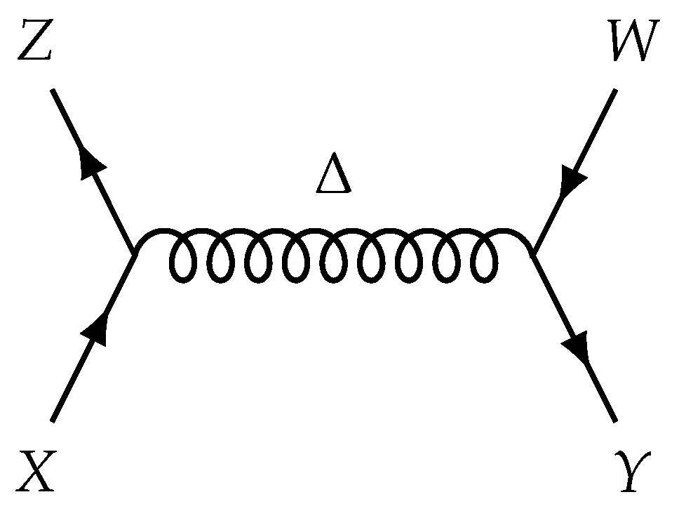
A general scheme of interactions between quarks can be depicted by a Feynman diagram, a sample of which is given in
Figure 2.
Straight lines with letters
X,
Y,
Z, and
W define quarks, a coiled line and the letter
define a gluon. Usually [
11] two quarks in the bottom are considered as income and two ones in top as result of interaction. Thus, the interaction depicted in
Figure 2 can be written as
. Lines of quarks are directed. Arrows pointing upwards (in the direction of reaction) denote quarks. Arrows pointing downwards (inverted direction of reaction) denote antiquarks, which can be treated as quarks moving back in time. So, according to this scheme,
X,
Z in the reaction
are quarks and
Y,
W are antiquarks. An essential rule here is that any gluon should contain color and anti-color. While drawing diagrams, this means that for each color unit traveling from left to right there should be a color unit moving in opposite direction.
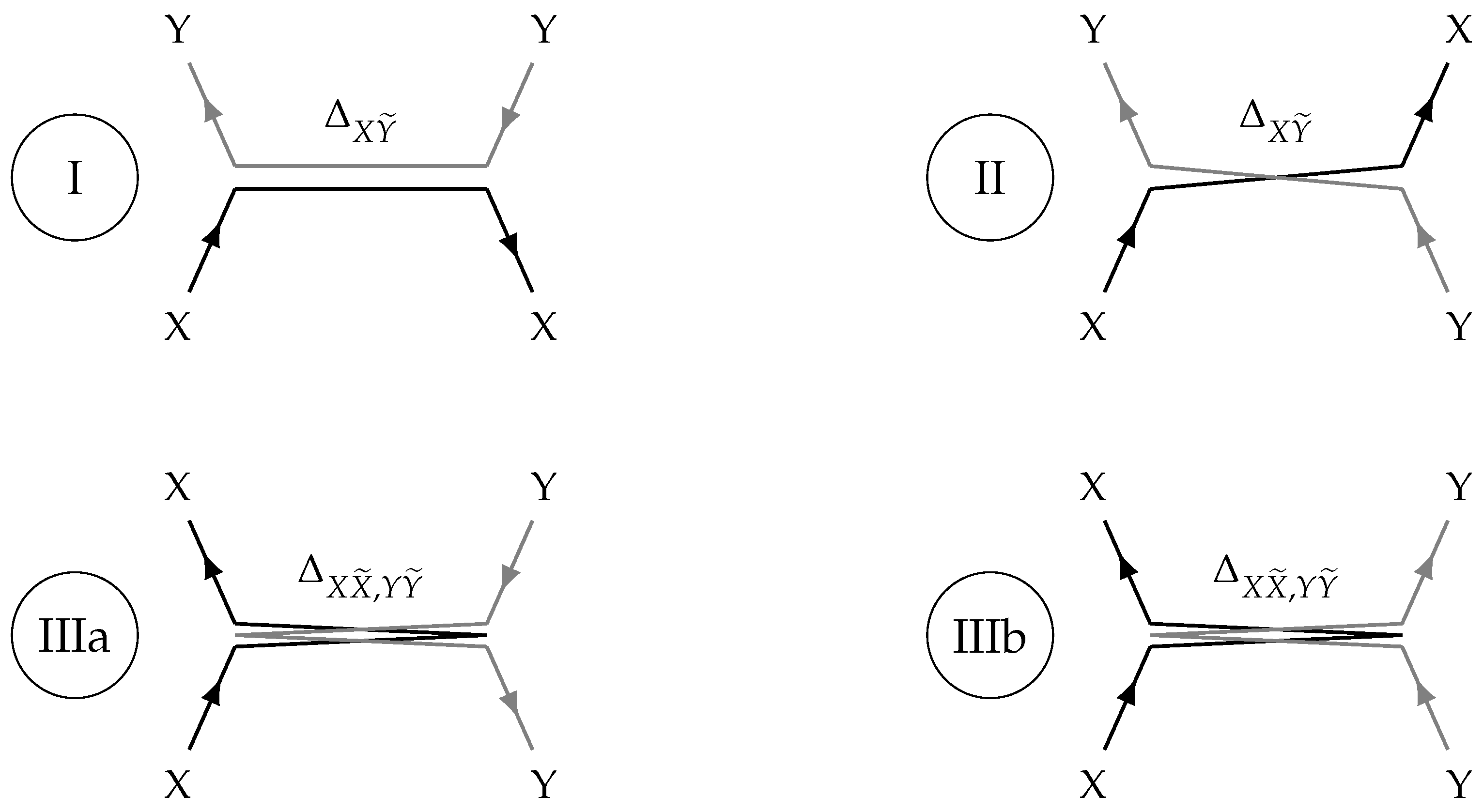
Figure 3 depicts the feasible schemes.
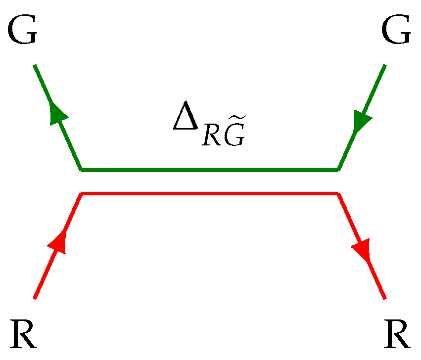
Consider the scheme I from
Figure 3, where
and
. Let
,
. This gives the reaction
, and the scheme I is customized to the one in
Figure 4.
In the left node the reaction
takes place. It can be written in matrix form as
and in compact operator form as
. The color coupling at this node is the coefficient at the right side of (
24):
.
Right node contains the reaction transforming anti-red quark to anti-green one:
. This is achieved by an antigluon, which is expressed by a conjugate matrix:
In compact form it is . The color coupling at this node is .
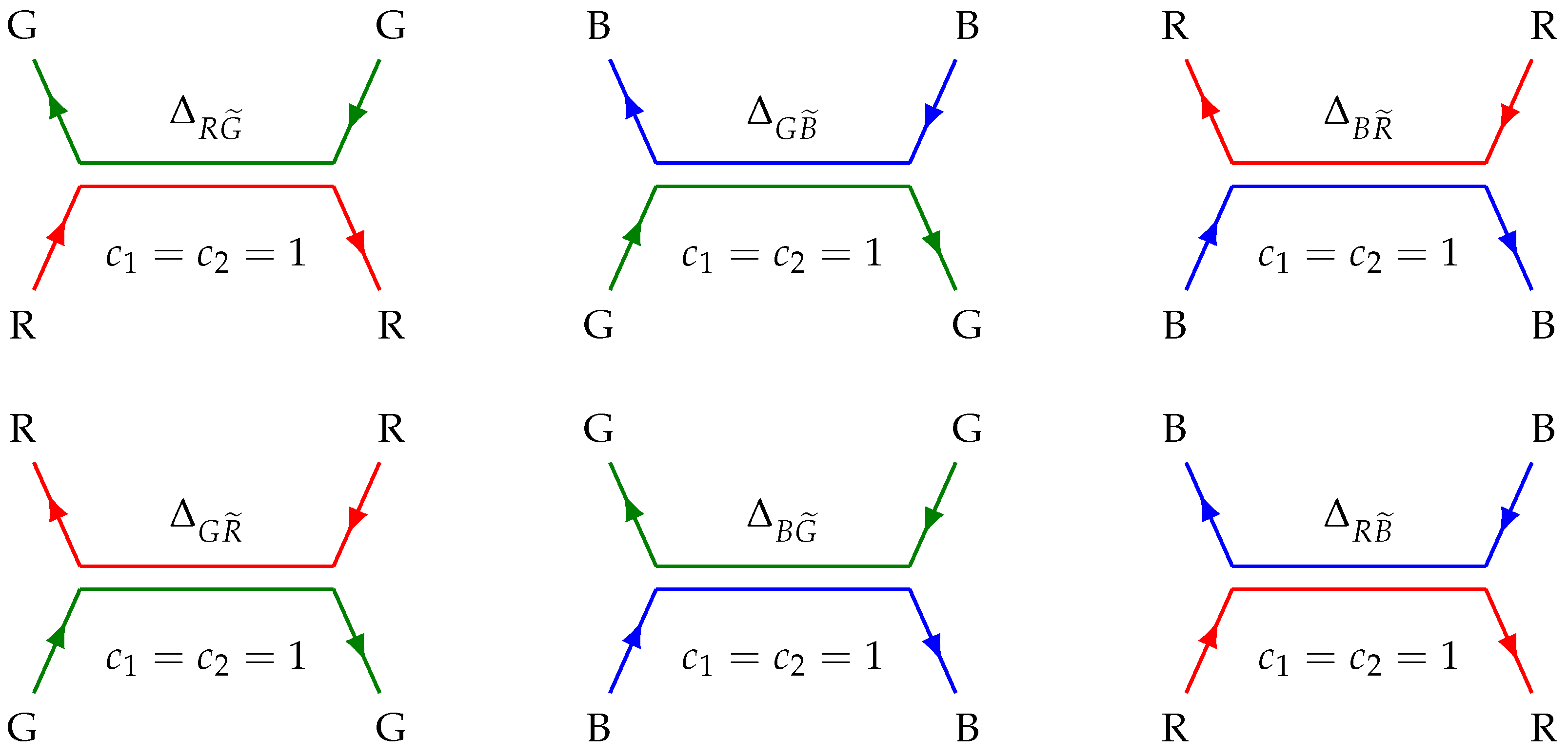
In QCD the magnitude of strong coupling in an exchange of a gluon between two color charges is proportional to the product of color couplings
and
, which are calculated at the vertices of the quark–gluon interaction [
11]. To calculate color multipliers let us consider all possible exchange processes between color charges with the participation of one out of eight gluons, which are described by (
22) and (
23). For the various color charges
R,
G,
B there occur the following exchange processes, effected with the aid of gluons of type (
22):
For the various anti-color charges
,
,
similar exchange processes take place, also brought about with gluons (
22):
The color coefficients in the above exchange processes appear as multipliers in the right-hand parts of the relations (
26) and (
27). Here, they all turn out to be equal to unit, i.e.,
. There are, in total, six variants of implementation of the scheme I,
. They are depicted in
Figure 5. The scheme I is not considered for
, this case if deferred to the scheme IIIa.
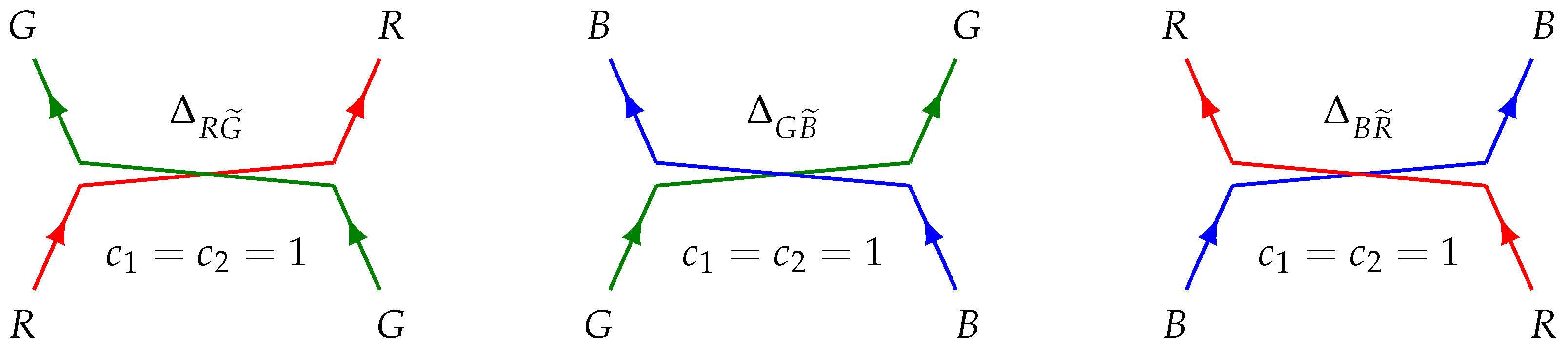
Consider the scheme II with
and
. Reactions from (
26) run in both nodes of the Feynman diagram and gluons (
22) are involved. Coupling coefficients are also all equal to unit. Three possible implementations are given in
Figure 6. Implementations for
, and
are just the same as in
Figure 6 with arrows going down and gluons replaced by antiparticles (conjugated matrices).
The scheme II is not considered for , this case if deferred to the scheme IIIb.
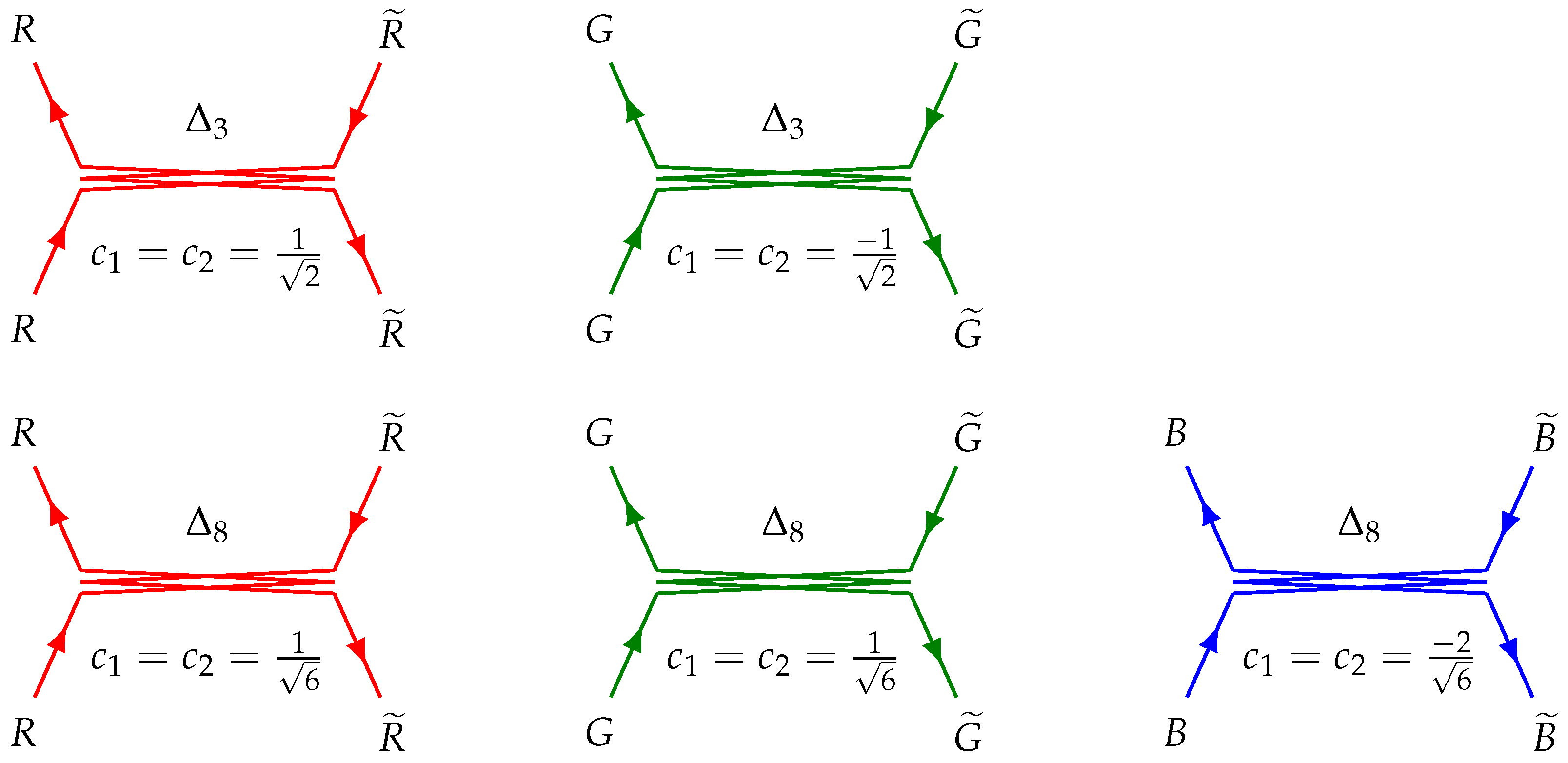
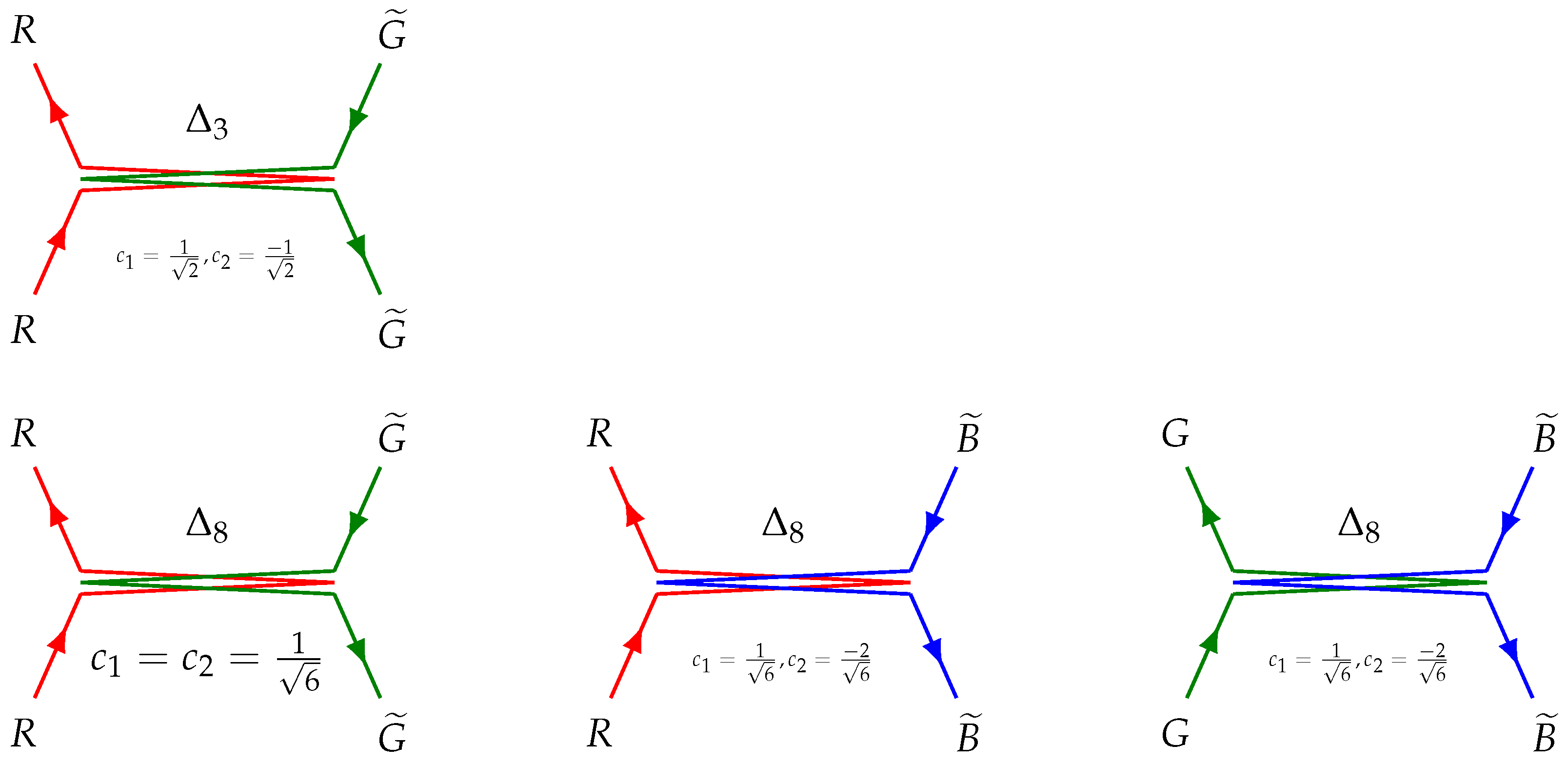
Now, consider the schemes IIIa and IIIb. They involve gluons (
23) rather than (
22). For these processes the following relations hold:
For anti-color charges analogously:
Implementations of the scheme IIIa with
are given in
Figure 7, and for
they are presented in
Figure 8.
Implementations of the scheme IIIb are alike to that of IIIa, except gluon stands in the right part of the diagrams, thus the arrows at the right part go in reverse direction. Due to the symmetry of (
23) matrices, this does not change the coupling coefficients.
6. Color Factors
Color factors of interactions between quarks are calculated [
11,
12] as
where
enumerates all possible channels of reaction. According to this,
Table 1 can be drawn for the symmetric case.
Any other interaction is same or similar to one of the above. For instance, G–R is same as R–G, B– is similar (by complex conjugation of its parts) to –R and therefore to R–.
To sum up, all interactions between quarks (of same or different color) have ; interactions between quarks and antiquark of same color have .
7. Alternative Antiquark Representation
There can be alternative way of introducing the antiquarks. Instead of conjugation as in (
13) one may consider defining antiquark as a vector negative to the corresponding quark:
In this representation, a contradiction appears in the scheme I. For instance, consider the interaction
depicted by
Figure 4. The left node does not contain antiquarks and presents the reaction
(
24) as before. However the reaction
in the right node with antiquarks (
31) becomes
Thus, the color factor is equal to zero and the reaction is not permitted. This is true for all reactions of scheme I as long as antiquarks are expressed as (
31). Scheme II does not include quark and antiquark together, schemes III are constructed for symmetric gluons (
23), so these schemes hold, and only scheme I should be excluded. As a result, the interactions between quark and antiquark of same color get
, making a uniform color factor in most of QCD reactions in bi-quark and tri-quark particles (mesons and barions); see the last column of
Table 1.
8. Permissible Types of Interactions between Gluon Pairs
The distinguishing feature of the QCD theory is that the gluons themselves carry a color charge and therefore may not only participate in exchange processes between quarks but interact with each other as well. However not any two gluons may enter an interaction, resulting in emerging of the third gluon. So, it is necessary to examine these processes in more detail. Each gluon is described by Hermitian operator of type (
22) or (
23). When two arbitrary chosen gluons
and
given by operators
and
, respectively, interact, they produce the third gluon
, which is described by the Hermitian operator
.
Although both
and
are Hermitian operators, their simple product
may be not. Otherwise, this introduces non-equality of the two interacting gluons. The simplest way to derive a resulting gluon is to take it as the anti-commutator:
where
c is the color coefficient calculated at the interaction vertex. It turns out that, for any gluons
and
, the left side of (
33) takes the form (
22), or (
23), or is zero. The latter case means the reaction is not permitted (or the coefficient
).
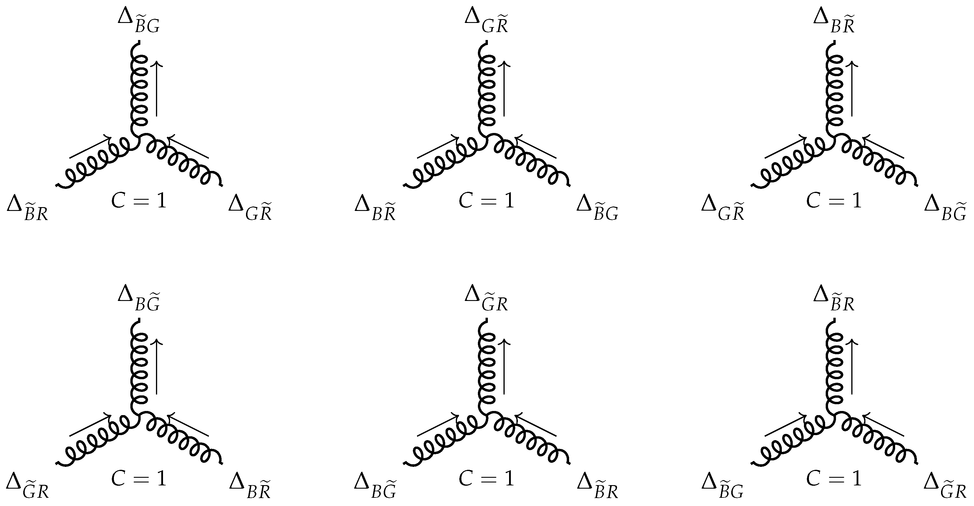
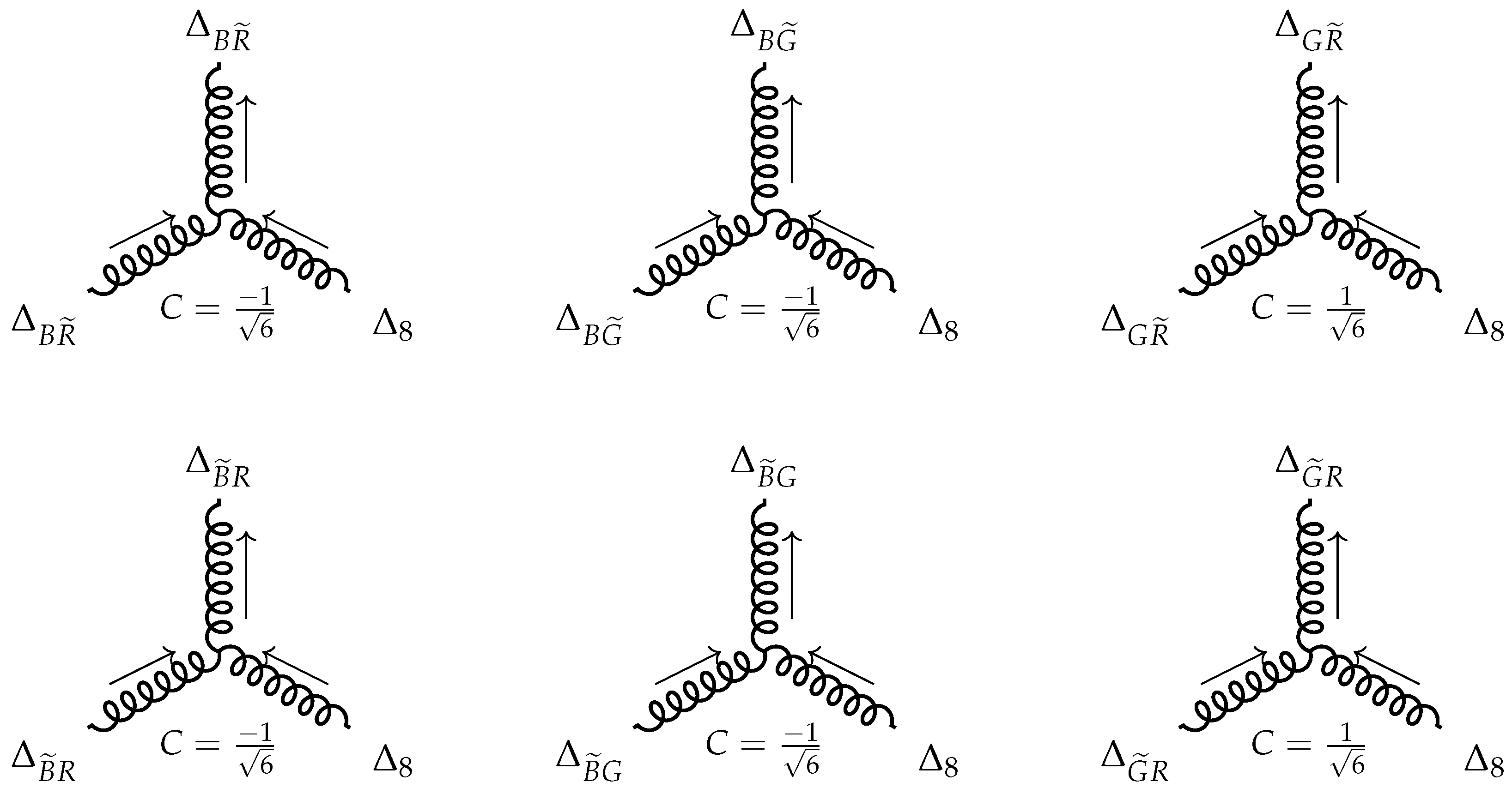
To begin with, consider the permissible variants of interaction of two gluons out of six from the set (
22). Here, 15 variants are possible and only six of them may take place in real interactions. They are shown in
Figure 9.
Make sure that this is possible with the sample of interacting
and
gluons. From (
33) it follows that
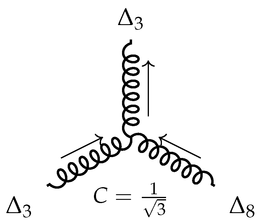
Consider now all the possible variants of a single interaction of gluon type (
22) with gluons from (
23). From (
33) we obtain six possible variants of interaction:
These interactions may be represented with diagrams in
Figure 10.
It should be noted that gluons of type (
22) do not interact with the gluon
. This gluon may only interact with
:
that is shown in
Figure 11.
Thus, we have considered all possible variants of one-time interaction of the eight gluons with each other and we have found the color coefficients corresponding to these interactions. This result enables regular manner construction of all permissible interactions of eight gluons with arbitrary multiplicity.
9. Conclusions
It is shown that, in contrast to the currently accepted approach, it is more natural to construct the theory of quantum chromodynamics on the basis of the group. This is the group of proper motions of the pseudo-Euclidean six-dimensional space or its isomorphic hyperbolic three-dimensional space, . This result is an indirect confirmation of the hypothesis that in microcosm our real physical space–time turns out to be the six-dimensional pseudo-Euclidean space . Furthermore, this supports the hypothesis of relationship between geometrical properties of the physical space–time with conserved physical quantum characteristics of elementary particles, particularly quarks.
The application of this theory is limited to the case of highly symmetrical six-dimensional space
containing three temporal dimensions. We suppose it exists in the microcosm of the scale below
cm, where strong interactions govern. In the bigger scale two of temporal dimensions are compacted [
7] and the space degrades to our usual
. This scale can be associated with the scale of quark confinement. The transform from
to
presumably occurs due to the curvature of space. The mathematics foundation here is to be studied.
There is a lot of potential to develop a six-dimensional theory, per se. Minkowski space
and its four-vector induce Poincare group of isometries, which correspond to the conservation laws. Analogously, the space
produces six-vector and a bigger group of isometries with additional conservation laws. Exploration of these laws started in the present work and in [
8] is to be continued.


