1. Introduction
Modeling using mathematical equations is critical in applied and basic science research. Moreover, it often leads to the formulation of new tasks and obtaining new scientific research results. In many areas, using mathematical and computational methods is crucial since their research subjects are often objects making it impossible or very difficult to perform natural experiments. Mathematical modeling of the studied thing allows experimenting with a tangible object to be replaced by purposeful research employing a mathematical model, thus allowing the experiment to be performed on the model using mathematical analysis and computer programs. Examining reality through abstract objects, appearing as models of high accuracy, is the essence of mathematical modeling.
Thus, mathematics, from a means of calculation, becomes a necessary modern research method. At certain stages it can be the only means of revealing the internal properties of the considered objects. Therefore, mathematical modeling applications can be defined as a practical approach to scientific research [
1,
2].
The current Special Issue can be given as an example of the great interest and activity of scientists in mathematical modeling applications in various scientific fields. It includes, among others, exciting applications in physics, topology, ecology, epidemiology [
3], and immunology [
4].
In particular, the paper [
4] considers a mathematical model describing the development of HIV infection. The central interacting populations are healthy T-cells, infected T-cells, and free HIV viruses. Their dynamics is described by ordinary differential equations (ODE). The authors perform a stability analysis of the model. For the numerical solution, they derive a modified continuous Galerkin–Petrov algorithm. The obtained results are compared with other numerical schemes.
Medicine is among the areas where mathematical modeling has been successfully applied in recent decades. Here, we propose a new model for the development of autoimmune diseases. Our goal is to analyze the role of some critical parameters of the model on the corresponding disorders. The remaining part of our paper is structured in the following sections. Some preliminaries describing the main immunological concepts are given in
Section 2.
Section 3 reviews some interesting recent applications of mathematical modeling in medicine and other fields. The modeling framework is introduced briefly. The proposed mathematical model is described in
Section 4.
Section 5 deals with numerical experiments.
Section 6 is devoted to conclusions and future scientific plans.
2. Basic Immunological Concepts
Human bodies are complex systems in which their cells and organs interact with foreign microorganisms. These interactions can be mutually beneficial, but they can also cause harm. Examples of valuable functions of various microorganisms, such as digestion, the participation in the production of some vitamins and foods, the detoxification of some harmful chemicals, and the strengthening of some immunological processes can be mentioned [
5,
6].
On the contrary, various pathogenic microscopic organisms, including viruses, bacteria, parasites, and fungi, can harm the host organisms. Examples of hazardous infectious diseases are Ebola virus hemorrhagic fever, cholera, polio, smallpox, human acquired immunodeficiency syndrome (HIV/AIDS), coronavirus disease (COVID-19), and many others [
7].
The defensive mechanisms in human organisms include external barriers, innate and acquired components, and secretions against foreign microorganisms. Collectively, they are called the immune system [
8].
One of the basic immunological concepts is that harmful foreign pathogens can directly attack cells, tissues, and organs but also affect the body’s protective functions and mechanisms [
5,
8]. One of the consequences is that the cause of death may not be an infection but the immune response to it [
5,
8].
Therefore, an essential property of a correctly functioning immune system must be its ability to discriminate between the cells and molecules of the host organism and foreign pathogens. The immune system should attack only pathogenic substances. Such an immune system is called tolerant to self [
9].
The concept of “self-nonself” is related to the clonal selection theory of M. Burnet and D. Talmage, the idea of the immunological homunculus of I. Cohen, and other theoretical concepts in immunology [
10].
When an immune system is not tolerant to its substances, it can start working against self components, leading to autoimmune disorders and diseases [
11].
The concept of auto-antibodies is related to the idiotype–anti-idiotype network theory of N. Jerne and other theoretical ideas by P. Ehrlich, etc. [
10].
The reasons for failures of proper functioning of the protection system and the occurrence of autoimmune disorders can differ: environmental factors, stress, genetics, diets, hygiene conditions (both bad and sound), etc. [
12,
13,
14]. Viruses have also been considered to be among the factors in the occurrence of autoimmune diseases [
15,
16,
17]. Strangely, some observations showed that sometimes viral infections could have a protective role from autoimmunity. To explain this, the so-called “hygiene hypothesis” was invented [
9].
Examples of autoimmune diseases, counting more than 80 diseases, are paroxysmal cold hemoglobinuria, lupus, multiple sclerosis, and rheumatoid arthritis [
18].
3. Mathematical Modeling in Medicine
Scientists use various research methods in treatment and health care. Clinical studies, laboratory investigations, qualitative health research, and quantitative methods are among them. Quantitative approaches apply statistical analyses, economic experiments, and computational and mathematical modeling methods to perform systematic and rigorous empirical studies [
19].
One of the most popular frameworks for the mathematical modeling of diseases is using systems of ordinary differential equations. Some recent models describe the development of autoimmune conditions [
20,
21,
22,
23,
24].
Another interesting approach is the modeling using fractional differential equations allowing the consideration of memory effects [
25,
26,
27,
28,
29,
30,
31]. During the last decade this approach has been successfully used for modeling the development of such diseases as HIV, COVID-19 and toxoplasmosis etc. [
28,
29,
31].
Long-distance travel has significantly increased for professional and tourist purposes in recent years. This change also leads to the possibility of the rapid spread of infections between people whose places of residence are located at great distances. A mathematical model describing such long-distance spread of diseases is proposed in the paper [
27]. The concept of superdiffusion is used to model such spreading. The authors present the basic notions and properties of fractional derivatives of noninteger order. Several ways of representing superdiffusion using fractional calculus are reviewed and compared concerning their ability to model the spread of infections over large distances.
The paper [
29] is devoted to a new mathematical model describing the development of toxoplasmosis disease in cats and people. The condition is caused by parasites called
Toxoplasma gondii. They can infect cats, and humans can also be infected after interactions with cats. The proposed mathematical model is described by a system of fractional differential equations. The authors provide essential information related to calculus using derivatives of fractional order. They describe the mathematical model in detail. The non-integer order paradigm is reviewed and applied to the analysis of the properties of the model. Qualitative analysis of the model is carried out, particularly stability analysis and sensitivity analysis concerning the primary threshold parameter of the model. The qualitative results are supported by the results of simulations performed with the use of a modified Adams–Bashforth–Moulton approach.
Another application of the fractional order calculus can be found in [
30], which studies the development of tuberculosis. The disease is caused by
Mycobacterium tuberculosis. Detailed information about the disease and its relation to other chronic conditions such as diabetes mellitus, HIV etc. is given. The authors provide a comparison between conventional and non-integer calculus and the possible advantages of each of them. Various areas of successful applications of fractional differentiation and integration are mentioned. The authors describe the basic concepts and properties of fractional derivatives. Further, they introduce the fractional order differential model describing the development of tuberculosis. The stability analysis of the model is performed. The conditions for existence and uniqueness of the model solutions are studied. Numerical simulations are carried out by applying a new predictor–corrector scheme. They confirm the qualitative results.
An application of fractional calculus to modeling the interactions between cancer and the immune system is proposed in the paper [
25]. The authors recall the primary factors and populations involved in tumor development and the host organism’s attempts to eradicate the disease. The authors mention the notion of the Caputo–Fabrizio derivative and describe its main properties. The mathematical model describing the interaction is presented and studied numerically applying a modified Adams–Bashforth approach. The role of the main parameters of the model is checked for the occurrence of chaos and oscillations.
The paper [
26] is devoted to applying fractional calculus to study the development of autoimmune diseases. The authors extend the model proposed in [
32] by applying the Caputo fractal-fractional operator. The problem of existence and uniqueness of the solution is studied. The researchers apply a numerical scheme using Lagrange interpolation to obtain approximate solutions. The role of various parameters of the model is studied numerically. The results of the simulations illustrate typical outcomes of autoimmune diseases.
Our paper uses a different approach: we apply the methodology used in statistical mechanics and generalized kinetic theory for active particles. This approach also considers the functional features of the interacting cells and particles. Additional variables perform the description of these states of activity. Examples of recent results using this methodology can be found in the papers [
20,
21,
22,
23,
33].
The considered system is divided into several of the most important populations of interacting individuals. Using concepts from the corresponding field of immunology, evolution equations for the concentrations of these populations are described including related gain and loss terms. They are integro-differential equations of the Boltzmann type. Further, qualitative and/or quantitative analysis can be performed.
In
Section 4, we introduce our mathematical model describing autoimmune diseases.
4. The Mathematical Model
By our study, we would like to investigate the meaning of the viral particles for developing autoimmune diseases.
Various mechanisms are known to cause autoimmune diseases, which are counted around 100 conditions today. Among these mechanisms is molecular mimicry, which can be caused by multiple viral infections [
5,
9]. Molecular mimicry can occur when peptides of some agents look like the host’s. This phenomenon may elicit immunological reactions against the foreign pathogens but also against components of the host possessing a similar protein structure or shape. In such a way a cross-reaction of the defense system with host antigens occurs, which may destroy the host’s constituents. The destroyed compartments may release additional isolated antigens that can be further attacked by the immunological cells. In this way we can observe continuous production of antigens that may become targets for the immune cells. Additionally, as a result, the autoimmune response may become solid and autodestructive.
In our mathematical model we consider the competition between four important populations:
- (i)
The first population of target cells;
- (ii)
The second population of damaged cells;
- (iii)
The third population of immune cells;
- (iv)
The fourth population of viral particles causing mimicry.
According to the mechanism of molecular mimicry, we suppose that some viruses activate immune responses destroying some healthy (target) cells.
We suppose that the organism can produce healthy cells that become target cells. We use a logistic-like gain term to model the rate of proliferation of the target cells.
Considering the most important features of the interactions between viruses and immune cells, we formulate four equations (one for the dynamics of each population) governing the system’s time evolution under consideration.
As a simplification of the reality, we suppose in our modeling process that the first two subsystems denoted by the labels and (corresponding to healthy (target) and destroyed cells) are unstructured; i.e. homogeneous concerning the activity. The populations denoted by and (corresponding to immunological cells and viruses) can function specifically in a non-homogeneous manner; i.e. they are structured populations. Their activities are represented by the variable . The meaning of the activities is as follows:
Immune cells: The activation state refers to their ability to destroy target cells.
Viruses: The activation state refers to their ability to trigger the production of immunological cells. Increasing values of the activation state denote higher amounts of newly produced immunological cells.
The states of the unstructured populations
and
are characterized, at time
t, by their concentrations
The states of the structured populations
and
are described by the probability densities
From the values of the probability densities it is possible to determine the concentrations of the structured populations as follows:
Our model is a generalization of previous models [
32,
34,
35] describing the development of autoimmune conditions. These models consider the populations of healthy (target) cells, damaged cells, immunological cells and viral particles.
The model [
32] is described using only ordinary differential equations. Therefore, the activation states of the populations are ignored.
The models [
32,
34] include the state of activity of immune cells. However, these models study the role of different model parameters.
In the present model, the activity of the virus particles is additionally introduced to study more aspects of the role of the pathogenicity of the virus infections for the autoimmune processes.
The modeling of the microscopic interactions between active particles of the various subsystems is performed by taking into account the variation rates of the amounts of active particles with corresponding inlet flux and outlet flux rates caused respectively by proliferative interactions (gain terms, GT) and outlet flux rates caused by destructive interactions (loss terms, LT) included in the general form of kinetic Equation (
4).
Thus, we obtain a specific representative of the general form of a kinetic type model as proposed in many foundational papers (e.g., [
36]) in the following way:
where stands for artificial influx of cells with activity u at time t.
As a result, the following system of ordinary and partial integro-differential equations is obtained:
with non-negative initial conditions
All parameters of the system (
5)–(
8) are assumed to be non-negative.
Equation (
5) describes the dynamics of the concentration
of the target cells. The meaning of the participating parameters is the following:
models the production rate of target cells from sources within the organism;
characterizes the rate of proliferation of the target cells;
refers to the concentration of the target cells at which their proliferation turns off;
describes the rate of the natural death of the target cells;
describes the damaging rate of the target cells attacked by the immune cells.
Equation (
6) models the time evolution of the concentration
of the damaged cells. The parameter
is the natural death rate of the damaged cells.
Equation (
7) describes the evolution of the distribution density
of the immune cells. The meaning of the participating parameters is the following:
is the rate of production of immune cells due to the presence of self-antigens presented by damaged cells;
is the rate of production of immune cells due to the presence of viruses;
is the rate of the natural death of the immune cells;
The factor is related to the assumption that the state of activity of the newly produced immune cells is low and they need time for activation.
Equation (
8) describes the evolution of the distribution density
of the viral particles. The meaning of the participating parameters is the following:
is the rate of production of viruses;
is the rate of destruction of the viruses due to the immune response;
is the rate of natural death of the viruses.
Let us introduce the following notation:
It can be shown that the following theorem holds.
Theorem 1. Let For each , there exists a unique solutionto the system (5)–(8) with the initial datum . The solution satisfies Proof. It is easy to check that the right-hand sides of the system (
5)–(
8) possess the property of Lipschitz continuity in the space denoted by
X. This guarantees that the solution exists and is unique locally. Further, by using the method of successive approximations, it can be shown that the solution is non-negative. Appropriate a priori estimations of the solution can be easily found. They are sufficient to have a unique solution on every finite temporary interval. □
5. Results of Simulations
The numerical algorithm for obtaining the approximate solution to the Cauchy problem corresponding to (
5)–(
8) includes the discretization of Equations (
7) and (
8) with respect to the activation states
by uniform meshes. The included integrals are approximated by using the composite Simpson’s rule.
The obtained system of ordinary differential equations has been solved for various parameter sets by the use of the solver
ode15s from the Matlab ODE suite [
37].
Due to the complexity of the considered nonlinear systems of ordinary differential equations obtained after the performed discretization, it is not possible to find analytically exact solutions of the models. For this purpose, Matlab’s ode15s solver based on the backward differentiation formulae proposed by Gear [
38] was used. The specificity of using such types of solvers is that the solver itself controls the accuracy of each step of the integration. It chooses the integration step so that the user-specified accuracy can be achieved. The values of relative tolerance RelTol and absolute tolerance AbsTol that we used are
and
. They provide an accuracy of 0.001 at any point in time. Such accuracy guarantees a good applicability and usability of the numerical results presented here.
It should be noted that in the course of the work a comparison was made between the results obtained by the program in the Matlab environment and those obtained by the multistep predictor–corrector method of Adams combined with the one-step Euler and Runge–Kutta methods, guaranteeing an accuracy of up to 0.001.
The assumption for the initial conditions has been that there is a certain amount of target cells, a small amount of damaged cells, and small amounts of immune cells with equally distributed states of activity and viruses with high states of activity:
The numerical experiments have been performed with the following values of parameters:
and various values of the parameter
.
The numerical experiments have been aimed at studying the effects of the damaging ability of the immune cells activated against target self-cells by viral infection.
In
Figure 1 and
Figure 2 the concentrations of target cells and damaged cells for small values of the parameters
and
are shown. This situation corresponds to weak immune system self-aggressivity when target cells remain at high levels and autoimmune disorders are not observed or are very mild.
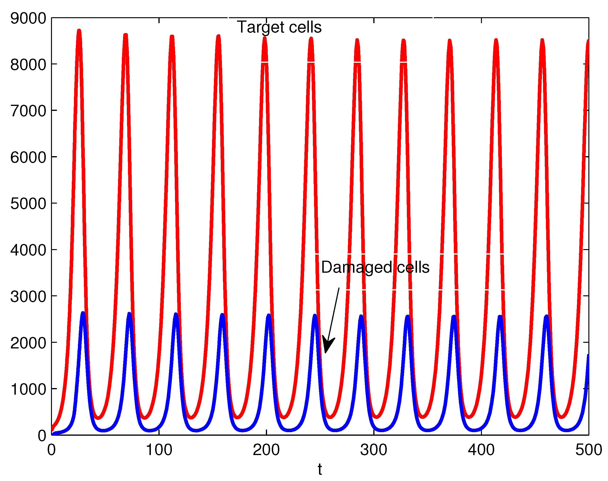
In
Figure 3,
Figure 4 and
Figure 5, respectively, results for higher values of the parameters
,
, and
are shown. This situation corresponds to strong self-aggressivity of the immune system when damping, periodic or increasing oscillations of the concentrations of target cells and damaged cells are observed. The cases of damping oscillations can be considered autoimmune disorders tending to some equilibrium states representing chronic diseases. Examples of chronic autoimmune diseases are type 1 diabetes and chronic immune thrombocytopenic purpura related to infection with the hepatitis C virus, which has been shown to be able to evade the immune response and to evolve into a chronic state in many infected patients [
24].
The cases with periodic and significantly increasing flare-ups can be considered autoimmune diseases characterized by repeated periods of dormancy of the autoaggressive immune cells and their flare-ups triggered by spreading pathogenic proteins, possible failure of regulatory immune cells to control the destructive reaction of effector immune cells against host constituents etc.; an example of repeated flare-ups is MS [
24]. The numerous repeated periods when large amounts of target cells are damaged can lead to severe tissue or organ destruction and even fatal results for the patients.


 ,
, 


