Article

Analysis of a Modified System of Infectious Disease in a Closed and Convex Subset of a Function Space with Numerical Study

1
Department of Mathematics, Lahore College for Women University, Lahore 54000, Pakistan
2
Department of Computer Science and Mathematics, Lebanese American University, Beirut 1102-2801, Lebanon
3
Department of Mathematics, Art and Science Faculty, Siirt University, 56100 Siirt, Turkey
4
Department of Mathematics, Mathematics Research Center, Near East University, Near East Boulevard, 99138 Nicosia, Turkey
5
Department of Mathematics, University of Management and Technology, Lahore 54000, Pakistan
6
Department of Mathematics and Statistics, The University of Lahore, Lahore 54000, Pakistan
7
Department of Humanities & Basic Sciences, MCS, National University of Sciences and Technology, Islamabad 44010, Pakistan
8
Department of Mathematics, Faculty of Science and Technology, University of Central Punjab, Lahore 54000, Pakistan
9
Department of Electricity and Electronics, Institute of Research and Development of Processes, Faculty of Science and Technology, University of the Basque Country, 48940 Leioa, Bizkaia, Spain
*
Author to whom correspondence should be addressed.
Axioms 2023, 12(1), 79; https://doi.org/10.3390/axioms12010079
Submission received: 5 December 2022 / Revised: 4 January 2023 / Accepted: 7 January 2023 / Published: 12 January 2023
(This article belongs to the Special Issue 10th Anniversary of Axioms: Mathematical Analysis)

Abstract

:
In this article, the transmission dynamical model of the deadly infectious disease named Ebola is investigated. This disease identified in the Democratic Republic of Congo (DRC) and Sudan (now South Sudan) and was identified in 1976. The novelty of the model under discussion is the inclusion of advection and diffusion in each compartmental equation. The addition of these two terms makes the model more general. Similar to a simple population dynamic system, the prescribed model also has two equilibrium points and an important threshold, known as the basic reproductive number. The current work comprises the existence and uniqueness of the solution, the numerical analysis of the model, and finally, the graphical simulations. In the section on the existence and uniqueness of the solutions, the optimal existence is assessed in a closed and convex subset of function space. For the numerical study, a nonstandard finite difference (NSFD) scheme is adopted to approximate the solution of the continuous mathematical model. The main reason for the adoption of this technique is delineated in the form of the positivity of the state variables, which is necessary for any population model. The positivity of the applied scheme is verified by the concept of M-matrices. Since the numerical method gives a discrete system of difference equations corresponding to a continuous system, some other relevant properties are also needed to describe it. In this respect, the consistency and stability of the designed technique are corroborated by using Taylor’s series expansion and Von Neumann’s stability criteria, respectively. To authenticate the proposed NSFD method, two other illustrious techniques are applied for the sake of comparison. In the end, numerical simulations are also performed that show the efficiency of the prescribed technique, while the existing techniques fail to do so.

1. Introduction

In 1976, the first case of Ebola virus disease was observed in the Democratic Republic of Congo (DRC). Ebola hemorrhagic fever is considered the most infectious deadly disease that is a member of the family “Filoviridae” and the genus “Ebola virus”. Ebola virus infect humans, bats, and monkeys, but species such as fawns and mice can also contract an infection. There are six types of Ebola virus, including Bundibugyo ebolavirus, Zaire ebolavirus, Sudan ebolavirus, Tai forest ebolavirus, Reston ebolavirus, and Bombali ebola virus. But only Bundibugyo ebolavirus, Zaire ebolavirus, Sudan ebolavirus and Tai forest ebolavirus are the source of infection in people, while Reston ebolavirus infects non-human primates [1,2,3].
This deadly disease has affected a large number of people globally. In the first wave of the disease in the DRC, the mortality rate was 88%, the number of exposed cases was 318, and 280 deaths were recorded. The second wave of the disease occurred in South Sudan, where the mortality rate, number of exposed cases, and total deaths were 53%, 284, and 151, respectively. After the first wave, Ebola virus disease occurred in several countries of the world, including Gabon, Guinea, Liberia, Sierra Leone, South Africa, Spain, Sudan, Uganda, the United Kingdom and the United States of America [4]. It is endemic in some parts of Africa.
In 1995, Ebola virus disease emerged again in the DRC with an estimation of 315 cases and 250 expired people. During 2014–2016, this epidemic re-emerged in West African countries. Approximately 11,300 people lost their lives, and 28,600 people were infected in Liberia, Guinea and Sierra Leone [5]. The case mortality rates in these countries were 42%, 60%, and 22%, respectively [6]. Approximately 2500 deaths were recorded in Guinea by May 2018. The Ugandan Ministry of Health confirmed the first case of Ebola virus disease on 11 June 2019; after that, the number of cases increased day by day. In 2019, about 2763 cases and 1841 deaths were reported in North Ituri and Kivu provinces, as confirmed by the DRC ministry of health [7]. According to recent figures, in 2020, 130 new infectious cases and 55 deaths were recorded, with a mortality rate of 42.3% in the Democratic Republic of Congo. However, the Ministry of Health and WHO declared on 18 November 2020 that the wave was terminated in the DRC [4]. In July 2016, Liberia was reported as Ebola-free.
The Ebola virus is transmitted to others by direct or indirect contact with infected individuals and animals. The bats-to-mammals route of transmission occurrs when land mammals eat fruits that were partially eaten by bats [8]. Initially, domestic and wild animals spread the virus to people. The human–human transference of the virus occurs through close contact with the infected person’s blood, tears, saliva, feces, bile, mucus, sweat, breast milk, urine, vomit, and spinal column fluid. The virus may also be transferred using needles and syringes contaminated by Ebola patients and by touching patients’ beds and clothes. People may contract an infection from an infected dead person during funeral rites without taking suitable precautions [9]. Unprotected healthcare workers may also contract an infection when treating the affected patients in hospitals and healthcare centers. The possibility of transmitting the virus increases among those people who look after their infected relatives.
During the infection period, the virus can be identified by an RT-PCR test or by immunological methods (ELISA) [10]. Usually, Ebola virus-infected persons show symptoms such as fever, fatigue, headache, bloody diarrhea, nausea, abdominal pain, loss of appetite, sore throat, and muscle pain [11]. The time from infection to the first appearance of symptoms is called the incubation period, which is normally 2 to 21 days for Ebola virus disease.
Mathematical modeling of the Ebola virus disease has been the concern of many researchers for the recent few years to understand the epidemiological and dynamical features of this challenging disease [12,13,14,15,16,17]. Weitz and Dushoff made control strategies to reduce the transmission of Ebola virus disease from infected dead bodies [18]. The researchers introduced and analyzed the optimal control mathematical problems by using various techniques and strategies for Ebola virus disease [19,20,21]. A. Mhlanga studied the two-patch model SIRD to study the dynamics of Ebola virus disease and developed time-dependent controls in his model. He calculated the basic reproductive number, the equilibrium points, and two boundary equilibria. He implemented the control measures to reduce the Ebola virus disease in specific areas [22]. Ahmed et al. [23] proposed the SEIR model with some new compartments, such as hospitalization, quarantine, and vaccination. In hospitalization and vaccination cases, optimal control strategies are used to control disease transmission and give the powerful impact of vaccination to the infected population. Tulu et al. introduced a mathematical model including quarantine and vaccination to analyze the disease dynamics [24]. They investigated the model using fractional-order derivatives and verified the existence and positive solution of their introduced model. They used Euler and Markov Chain Monte Carlo (MCMC) methods to generate the simulations. Their outcomes illustrated that the quarantine and vaccinations played an important part to control the Ebola outbreak. Area et al. presented a mathematical model with the vaccination of susceptible individuals to control disease transmission [25]. They studied two optimal control problems associated with Ebola disease transmission with vaccination. They considered three vaccination constraints to show the impact of vaccination. A SIR model was constructed with direct and indirect transmissions by Berge et al. [26]. They proved the local and global asymptotic stability of the endemic equilibrium points and developed the nonstandard finite difference scheme, which is dynamically consistent with the model. Kabli et al., in 2018, used the cooperative systems theory to examine the global stability of the epidemic SEIHR model of Ebola disease [27]. Rafiq et al., in 2020, constructed an SEIR model of nonlinear differential equations [28]. They obtained the threshold quantity and equilibrium points and checked the stability of their proposed model. They proved that the equilibrium points are locally asymptotically stable. The Lyapunov function was used to check the global stabilities. They developed a fourth-order Runge–Kutta method and a nonstandard finite difference scheme for the proposed model and demonstrated that the RK-4 method failed at certain step sizes, while the NSFD scheme conserved all the dynamical properties of the model at large step sizes. Okyere et al. examined the optimal control analysis of epidemiological models such as SIR and SEIR using vaccination, treatment, and educational campaigns as time-dependent control functions [29]. They used the forward-backward sweep method with the RK-4 method to explain the optimal system for different control strategies. Ahmed et al. [30], in 2020, established a mathematical model SVEIR by introducing the new sub-population class of vaccinated people into the SEIR model [31]. They also presented the equilibrium points and stability analysis of the model. Both the disease-free and endemic equilibrium points are locally and globally stable. They justified their concluded theoretical outturn by applying RK-4 and NSFD schemes. Their work shows that through voluntary vaccinations, the transmission of the Ebola virus can be controlled. A work regarding a fuzzy epidemic model with an NSFD scheme is presented by Dayan et al. [32].
Some innovative studies for epidemic models in the set of fractional calculus have been conducted. The referred articles are of importance in this connection [33,34]. In the existing theories, advection and diffusion phenomena are considered for the propagation of disease in the defined population. The existing epidemic models deal with the disease dynamics depending on time. However, they do not examine the effect of advection and diffusion factors simultaneously. For that reason, there is no numerical design for this type of model in the running literature, which is, in this context, the generalized epidemic Ebola model, namely the advection–diffusion Ebola model. Moreover, the existing numerical schemes do not preserve the positivity property, which is the essential feature of the solutions to the population systems. Additionally, they lead toward a false steady state. This was a major drawback in some of the present numerical designs. The scheme proposed and developed in this article ensures positive solutions, stability, and convergence toward the true steady state. Hence, the extended model is productive and enriched with disease dynamics.
As far as the limitations of the research work are concerned, the initial and boundary conditions of the underlying model should be continuous functions. If these conditions are discontinuous, piecewise continuous, or nonlocal conditions, then they cannot be considered. The other limitation is related to the existence and uniqueness of the solution. The continuity of the solution lies in a restricted domain. Equivalently, the maximum length of continuity is short.

2. Modified Ebola Virus Model

A compartmental model of the Ebola virus is designed for the numerical study in Section 2. The model under study deals with the spatio-temporal dynamics of the Ebola virus disease. Due to the involvement of space as well as time, the domain for the current model is assumed to be Ω = ( 0 , L ) × ( 0 , T ) R 2 , where L and T are real numbers, such that T > 0 . Suppose that the state variables for the system are S = S ( x , t ) , E = E ( x , t ) , I = I ( x , t ) , and R = R ( x , t ) , which are the real functions defined on Ω and are described as the subpopulation sizes of the compartments susceptible, exposed, infected, and recovered, respectively, at any time t. Further, let S = S ( x , t ) , E = E ( x , t ) , I = I ( x , t ) , R = R ( x , t ) C 2 , 1 [ Ω , R ] . Additionally, suppose that ζ 1 ( x ) , ζ 2 ( x ) and ζ 3 ( x ) are three real-valued functions such that ζ 1 ( x ) , ζ 2 ( x ) , and ζ 3 ( x ) C 1 [ ( 0 , L ) , R ] . The state variables of the model and parameters used in the prescribed system are stated in Table 1.
The spatio-temporal model of Ebola virus disease including advection and diffusion is given as follows [35]:
S ( x , t ) t + a 1 S ( x , t ) x = p 1 p 2 S ( x , t ) E ( x , t ) p 1 S ( x , t ) + δ 1 d 2 S ( x , t ) d x 2 ,
E ( x , t ) t + a 2 E ( x , t ) x = p 2 S ( x , t ) E ( x , t ) p 3 E ( x , t ) p 1 E ( x , t ) + δ 2 d 2 E ( x , t ) d x 2 ,
I ( x , t ) t + a 3 I ( x , t ) x = p 3 E ( x , t ) ( p 1 + p 4 ) I ( x , t ) + δ 3 d 2 I ( x , t ) d x 2 ,
R ( x , t ) t + a 4 R ( x , t ) x = p 4 I ( x , t ) p 1 R ( x , t ) + δ 4 d 2 R ( x , t ) d x 2 .
Since all of the above equations are independent of R ( x , t ) , thus, the system (1)–(4) reduces to the system of the first three Equations (1)–(3).
S ( x , t ) t + a 1 S ( x , t ) x = p 1 p 2 S ( x , t ) E ( x , t ) p 1 S ( x , t ) + δ 1 d 2 S ( x , t ) d x 2 ,
E ( x , t ) t + a 2 E ( x , t ) x = p 2 S ( x , t ) E ( x , t ) p 3 E ( x , t ) p 1 E ( x , t ) + δ 2 d 2 E ( x , t ) d x 2 ,
I ( x , t ) t + a 3 I ( x , t ) x = p 3 E ( x , t ) ( p 1 + p 4 ) I ( x , t ) + δ 3 d 2 I ( x , t ) d x 2 .
Additionally, the initial and boundary conditions
S ( x , 0 ) = ζ 1 ( x ) , for all x [ 0 , L ] ,
E ( x , 0 ) = ζ 2 ( x ) , for all x [ 0 , L ] ,
I ( x , 0 ) = ζ 3 ( x ) , for all x [ 0 , L ] ,
and
S ( x , t ) η = E ( x , t ) η = I ( x , t ) η = 0 ,
for every ordered pair ( x , t ) Ω , η represent outward normal derivatives on Ω , a boundary of Ω where η is the outward unit normal vector on the boundary. Furthermore, S ( x , t ) , E ( x , t ) , I ( x , t ) , R ( x , t ) are Lebesgue-integrable functions in the domain mentioned above.
The prescribed system (1)–(4) reflects the dynamical behaviour of the fatal Ebola virus disease, for which S ( x , t ) , E ( x , t ) , I ( x , t ) and R ( x , t ) depict the sub-population sizes of respective compartments at point x and time t, respectively. Due to biological reasoning, it is assumed that S , E , I and R are the nonnegative functions of x and t [36,37,38].
For the equilibrium points, set all instantaneous changes with respect to time and space equal to zero in (5)–(7).
Thus, the Ebola-free equilibrium point of the continuous system is:
E 0 = ( 1 , 0 , 0 , 0 ) .
Additionally, the endemic equilibrium of the model, obtained by equating all derivatives to zero, is [35]:
E e = ( S ˜ , E ˜ , I ˜ , R ˜ ) ,
where S ˜ = p 1 + p 3 p 2 , E ˜ = p 1 ( 1 S ˜ ) p 2 S ˜ , I ˜ = p 3 E ˜ p 1 + p 4 , R ˜ = p 4 I ˜ p 1 .
Additionally, the value of the reproductive number R 0 can be evaluated by using a next-generation matrix.
E I = p 2 S 0 0 0 E I p 3 + p 1 0 p 3 p 1 + p 4 E I .
Since S = 1
F = p 2 0 0 0 , V = p 3 + p 1 0 p 3 p 1 + p 4 .
Because R 0 is defined as the spectral radius of F V 1 , thus,
R 0 = ρ ( F V 1 ) , = p 2 p 1 + p 3 .
To make the dynamical system more realistic, many researchers examined advection and diffusion phenomena in highly non-linear continuous mathematical models, which reflect the real significance in the dynamics of the systems [39,40]. The current article addresses the advection and diffusive impacts of an epidemic model’s compartmental population.
The approach of the nonstandard finite difference scheme for the model (1)–(4) is adopted with the defined initial and boundary conditions in the next section with the supplementary data (8)–(11).

2.1. Optimal Analysis of the Model

The above system (1)–(4) of Ebola disease and its dynamics depend upon the advection and diffusion properties with respect to each of the state variables S , E , I , and R. The first three partial differentials are mutually coupled, while the last partial differential Equation (4) is completely independent of the rest of the coupled system. Since this model primarily describes the population model, where the sum S + E + I + R = N (the total population), therefore, physically, if the total population is known, the three components are computed from the partial differential Equations (1)–(4). Then, obviously, the fourth tuple of the vector of unknown functions is retained without computing the fourth partial differential Equation (4). Thus, potentially, Equation (4) can be set aside for the upcoming existence analysis, the same as it is in the computations. Now, we will consider System (1)–(3) with the conditions (8)–(11). Without any inconvenience, the first time derivative appearing in the system can be inverted, and in concise form, the solutions S , E , I can be written as follows:
S = S 0 + 0 t ϝ 1 S , E , I , S x , 2 S x 2 ( s ) d s , E = E 0 + 0 t ϝ 2 S , E , I , E x , 2 E x 2 ( s ) d s , I = I 0 + 0 t ϝ 3 S , E , I , I x , 2 I x 2 ( s ) d s .
If we set S , E , I = u 1 , u 2 , u 3 , the more compact form of System (1)–(4) and, consequently, Equations (5)–(7) can be written as:
u i t = ϝ i u 1 , u 2 , u 3 , u i x , 2 u i x 2 ,
where u 1 , u 2 , u 3 , i = 1 , 2 , 3 represent the unknown functions S , E , and I, respectively.
The classical triple u 1 , u 2 , u 3 needs to be in the function space C 1 [ 0 , T ] × C 2 [ a , b ] for finite numbers a , b and the finite positive number T . The compact embedding of the function spaces leads to the fact that the function space C 1 [ 0 , T ] is compactly embedded as C 0 [ 0 , T ] ; consequently, we can have the consideration of the space of continuous functions as our primary Banach space for the solution tuple to be fit in the space C 0 [ 0 , T ] , equipped with the usual supremum norm. Furthermore, we strictly assume that, with respect to the space variable, this u i C 2 [ a , b ] for i = 1 , 2 , 3 , that is, we invert System (12) with the initial conditions (8)–(10) in the form of the Volterra integral equation as follows:
u i = u 0 i + 0 t ϝ i u 1 , u 2 , u 3 , u i x , 2 u i x 2 ( s ) d s , for i = 1 , 2 , 3 .
The integral Equation (13) can be written in the following operator’s form:
U i = u 0 i + 0 t ϝ i u 1 , u 2 , u 3 , u i x , 2 u i x 2 ( s ) d s , for i = 1 , 2 , 3 .
Since System (1)–(4) reduced to (14) is a physical system, prior to the computational technique, we can predict the behaviour of the solution. Besides the many advantages of the existence theory, there is one serious restriction, which is that, in general, the solution does not exist in the large domain. However, we can construct an a priori condition on the bound of the solution in a special environment called the Schauder-type estimates. This fact leads to the nice idea of the optimization of the function space. The following subsection deals with the important dimension of the analysis.

Fixed-Point Optimization in Banach Spaces

Primarily, we will consider the contraction-mapping principle on the space of continuous functions, and we choose the following balls with arbitrary radii r > 0 (to be bounded later) defined by
B r i [ u 0 i ] = u i C 0 [ 0 , ρ ] , u i u 0 i r i , i = 1 , 2 , 3 .
We choose the initial values as the center of the balls, and we set
u i r i + u 0 i .
Again, considering the operator Equation (14), we examine the following conditions:
(i)
Self-mapping; that is, U i : B r [ u 0 i ] B r [ u 0 i ] ,
(ii)
Contractivity; that is, U 1 i U i 2 k i u 1 i u 2 i .
To verify the first condition, we take the norm of Equation (14), and we obtain
U i u 0 i 0 t ϝ i d r ,
K i ( r ) 0 t d s , because ϝ i are bounded and the norm can be estimated by the radius r .
K i ( r ) ρ , r .
This implies that
ρ r K i ( r )
The condition (16) is necessary for the existence of a solution and gives explicit bounds for the length of the continuity of intervals of solutions. For contractivity, we take two images U 1 i and U 2 i for two pre-images u 1 i and u 2 i , respectively, from (14), and we can rewrite this as follows:
U 1 i U 2 i = 0 t ϝ i u 1 i , u 1 i t , 2 u 1 i t 2 ( s ) d s 0 t ϝ i u 2 i , u 2 i x , 2 u 2 i x 2 ( s ) d s , U 1 i U 2 i = 0 t ϝ i u 1 i , u 1 i x , 2 u 1 i x 2 ϝ i u 2 i , u 2 i x , 2 u 2 i x 2 ( s ) d s .
Now, suppose that ϝ i , i = 1 , 2 , 3 all satisfy the Lipschitz condition of spatial type as defined by
ϝ i ( u 1 i ) ϝ i ( u 2 i ) L i ( r ) u 1 i u 2 i C 2 [ a , b ] .
Equation (17) implies
U i i U 2 i ρ L i ( r ) u 1 i u 2 i C 2 [ a , b ] ,
and for some positive constant M i , we can always have
U i i U 2 i ρ M i L i ( r ) u 1 i u 2 i C 2 [ a , b ] .
For contractivity, we have the following condition:
ρ < 1 M i L i ( r ) ,
that is, we have more restrictions on the length of the interval of continuity depending on time. For more precise results, the Lipschitz constant must be small enough.
Hence, the following result has been verified.
Theorem 1. 
Suppose that the state variables S , E , I and R are in C 1 [ 0 , T ] × C 2 [ a , b ] ; then, provided that S , E , I and R satisfy the Lipschitz condition of the type of Equation (18), the initial boundary value problem (1)–(4) with (8)–(11) is uniquely solvable.
Theorem 2. 
Suppose that the state variables S , E , I and R are in C 1 [ 0 , T ] × C 2 [ a , b ] ; then, the continuity and the uniqueness of the solution of System (1)–(4) is given by the inequality,
ρ < r k i ( r ) = 1 M i L i ( r ) .
Since the epidemic models contain a number of parameters, it becomes an uphill task to find the exact solutions of these models. In some cases, it even becomes impossible to evaluate the problem exactly. The numerical solutions then numerical solutions become inevitable for these types of nonlinear epidemic systems.
In the subsequent section, a non-standardized algebraic scheme is designed to attain the numerical solutions of the underlying model.

2.2. Numerical Modeling

Let M and M * be two natural numbers and m = L M , = T M * be the positive real numbers. Additionally, let [ 0 , L ] and [ 0 , T ] be the spatial and temporal intervals, respectively, for the proposed problem. Thus, the intervals [ 0 , L ] and [ 0 , T ] are partitioned into m and subintervals, respectively. Suppose also that the partition norm of the interval [ 0 , L ] is m, while the partition norm for the interval [ 0 , T ] is . Define x j = j m and t k = k , for which j { 0 , 1 , 2 , M } and k { 0 , 1 , 2 , M * } . Additionally, suppose that S j k , E j k , I j k , and R j k are the approximate values of the exact values of the functions S ( x j , t k ) , E ( x j , t k ) , I ( x j , t k ) , and R ( x j , t k ) respectively, at the mesh point ( j m , k ) for j Z and 0 j M and k Z and 0 j M * . Additionally, if U is the arbitrary function values from the set { S , E , I , R } , then we define
U k = ( U 0 k , U 1 k , , U M k ) , k Z and 0 j M * .
The continuous model (1)–(3) is converted in to a system of difference equations with the help of some discrete functions. The procedure of conversion is explained as follows:
S j k + 1 S j k + a 1 S j k + 1 S j 1 k + 1 m = p 1 p 2 S j k + 1 E j k p 1 S j k + 1 + δ 1 S j + 1 k + 1 2 S j k + 1 + S j 1 k + 1 m 2 ,
E j k + 1 E j k + a 2 E j k + 1 E j 1 k + 1 m = p 2 S j k E j k p 3 E j k + 1 p 1 E j k + 1 + δ 2 E j + 1 k + 1 2 E j k + 1 + E j 1 k + 1 m 2 ,
I j k + 1 I j k + a 3 I j k + 1 I j 1 k + 1 m = p 3 E j k ( p 1 + p 4 ) I j k + 1 + δ 3 I j + 1 k + 1 2 I j k + 1 + I j 1 k + 1 m 2 .
After simplifications, (20)–(22) gives
( λ 1 + μ 1 ) S j 1 k + 1 + ( 1 + λ 1 + p 1 + p 2 E j k + 2 μ 1 ) S j k + 1 μ 1 S j + 1 k + 1 = p 1 + S j k ,
( λ 2 + μ 2 ) E j 1 k + 1 + ( 1 + λ 2 + ( p 1 + p 3 ) + 2 μ 2 ) E j k + 1 μ 2 E j + 1 k + 1 = E j k + p 2 S j k E j k ,
( λ 3 + μ 3 ) I j 1 k + 1 + ( 1 + λ 3 + ( p 1 + p 4 ) + 2 μ 3 ) I j k + 1 μ 3 I j + 1 k + 1 = I j k + p 3 E j k ,
where λ 1 = a 1 m , μ 1 = δ 1 m 2 , λ 2 = a 2 m , μ 2 = δ 2 m 2 , λ 3 = a 3 m and μ 3 = δ 3 m 2 for j { 1 , 2 , , M } and k { 0 , 1 , 2 , , M * 1 } .
The auxiliary data are discretized as:
S j 0 = k 1 ( x j ) , E j 0 = k 2 ( x j ) , I j 0 = k 3 ( x j ) , for j { 1 , 2 , , M } ,
and
δ S 1 k = δ E 1 k = δ I 1 k = 0 , δ S M k = δ E M k = δ I M k = 0 , for k { 0 , 1 , 2 , , M * } .
A comparison of numerical scheme (20)–(22) with the other existing methods makes it clear that (20)–(22) gives us more reliable results. Thus, to see the strength of our proposed scheme, two well-known schemes are also applied to the proposed system (1)–(3). One is the up-wind implicit scheme, which is constructed as
( λ 1 + μ 1 ) S j 1 k + 1 + ( 1 + λ 1 + 2 μ 1 ) S j k + 1 μ 1 S j + 1 k + 1 = S j k + p 1 p 2 S j k E j k p 1 S j k ,
( λ 2 + μ 2 ) E j 1 k + 1 + ( 1 + λ 2 + 2 μ 2 ) E j k + 1 μ 2 E j + 1 k + 1 = E j k + p 2 S j k E j k p 3 E j k p 1 E j k ,
( λ 3 + μ 3 ) I j 1 k + 1 + ( 1 + λ 3 + 2 μ 3 ) I j k + 1 μ 3 I j + 1 k + 1 = I j k + p 3 E j k p 4 I j k p 1 I j k .
The second is the Crank–Nicolson method, constructed for System (1)–(3):
λ 1 4 + μ 1 2 S j 1 k + 1 + ( 1 + μ 1 ) S j k + 1 + λ 1 4 μ 1 2 S j + 1 k + 1 = λ 1 4 + μ 1 2 S j 1 k + 1 p 2 E j k p 1 μ 1 S j k + μ 1 2 λ 1 4 S j + 1 k + p 1 ,
λ 2 4 + μ 2 2 E j 1 k + 1 + ( 1 + μ 2 ) E j k + 1 + λ 2 4 μ 2 2 E j + 1 k + 1 = λ 2 4 + μ 2 2 E j 1 k + 1 + p 2 S j k p 3 p 1 μ 2 E j k + μ 2 2 λ 2 4 E j + 1 k ,
λ 3 4 + μ 3 2 I j 1 k + 1 + ( 1 + μ 3 ) I j k + 1 + λ 3 4 μ 3 2 I j + 1 k + 1 = λ 3 4 + μ 3 2 I j 1 k + 1 p 4 p 1 μ 3 I j k μ 3 2 λ 3 4 I j + 1 k + p 3 E j k .
Remark 1. 
The proposed NSFD scheme can be developed by taking unequal step sizes of both time and space.

3. Physical Features of the Numerical Method

This portion is fixed for the significant characteristics of System (5)–(7). These features play a paramount role to attain the numerical solutions of the nonlinear epidemic models. To discuss these important features, it is important to review some definitions.
Definition 1. 
A matrix A with real entries is described as a Z-matrix if every element of it is non-positive except diagonal elements.
Definition 2. 
A square matrix A with real entries is described as an M-matrix if it satisfies the following properties:
(i) 
The matrix A is a Z-matrix;
(ii) 
Every main diagonal entry of the matrix A is positive;
(iii) 
The matrix A is diagonally dominated, strictly.
The theory of the M-matrix plays an important role in proving the positivity of the state variables involved in the model of various fields of engineering, mathematics, economics, physics, and many more. The subsequent outcome grantees the non-negativity of the numerical solutions to the discrete System (20)–(22). This feature of the numerical scheme can be expressed by applying the M-matrix technique. Moreover, every M-matrix is inverted with real positive entries.
Remark 2. 
Every M-matrix has an inversion with positive entries [41].
The following are the important properties of the proposed scheme for the model under discussion.

3.1. Positivity

For a population dynamical system, the positivity of the state variables plays a vital role. Thus, it must be preserved after employing the numerical scheme on the model. The following theorem reflects the positivity property.
Theorem 3. 
Assume that k 1 , k 2 and k 3 are the positive real-valued functions depending on x defined in the interval ( 0 , L ) ; then, System (20)–(22), with the supportive data (8)–(11), has a solution ∀ m > 0 and l > 0 . Moreover, the solutions are positive.
Proof. 
Since the left hand sides of (20)–(22) are the implicit relations, we can write it in the vector representation as:
U S k + 1 = S j k + p 1 ,
V E k + 1 = E j k + p 2 S j k E j k ,
W I k + 1 = I j k + p 3 E j k ,
in which U , V and W are defined as ( M + 1 ) × ( M + 1 ) matrices. By using the initial and boundary conditions (8)–(11), we can find the matrices U , V and W. Then,
U = ( γ 1 ) 0 k γ 2 0 0 γ 3 ( γ 1 ) 1 k γ 4 0 γ 3 ( γ 1 ) 2 k γ 4 γ 3 ( γ 1 ) M 2 k γ 4 0 γ 3 ( γ 1 ) M 1 k γ 4 0 0 γ 3 ( γ 1 * ) M k ,
V = ( ξ 1 ) 0 k ξ 2 0 0 ξ 3 ( ξ 1 ) 1 k ξ 4 0 ξ 3 ( ξ 1 ) 2 k ξ 4 ξ 3 ( ξ 1 ) M 2 k ξ 4 0 ξ 3 ( ξ 1 ) M 1 k ξ 4 0 0 ξ 3 ( ξ 1 * ) M k ,
and
W = ( ϱ 1 ) 0 k ϱ 2 0 0 ϱ 3 ( ϱ 1 ) 1 k ϱ 4 0 ϱ 3 ( ϱ 1 ) 2 k ϱ 4 ϱ 3 ( ϱ 1 ) M 2 k ϱ 4 0 ϱ 3 ( ϱ 1 ) M 1 k ϱ 4 0 0 ϱ 3 ( ϱ 1 * ) M k ,
where
( γ 1 ) j k = 1 + λ 1 + p 1 + p 2 E j k + 2 μ 1 , ( ξ 1 ) j k = 1 + λ 2 + ( p 1 + p 3 ) + 2 μ 2 , ( ϱ 1 ) j k = 1 + λ 3 + ( p 1 + p 4 ) + 2 μ 3 , ( γ 1 * ) M k = 1 + λ 1 + p 1 + p 2 E M k + μ 1 , ( ξ 1 * ) M k = 1 + λ 2 + ( p 1 + p 3 ) + μ 2 , ( ϱ 1 * ) M k = 1 + λ 3 + ( p 1 + p 4 ) + μ 3 ,
γ 2 = ( λ 1 + 2 μ 1 ) , ξ 2 = ( λ 2 + 2 μ 2 ) , ϱ 2 = ( λ 3 + 2 μ 3 ) , γ 3 = ( λ 1 + μ 1 ) , ξ 3 = ( λ 2 + μ 2 ) , ϱ 3 = ( λ 3 + μ 3 ) , γ 4 = μ 1 , ξ 4 = μ 2 , ϱ 4 = μ 3 .
Now, the method of mathematical induction is applied to prove the positivity of the corresponding discrete system of Equations (20)–(22). According to the initial data, S 0 , I A 0 and I C 0 are positive, so it is assumed that S k , E k and I k , k 0 , 1 , 2 , , M * 1 are positive component vectors. The above calculation indicates that U , V , and W are the M-matrices, so they are invertible and have positive inverses. Moreover, the expressions that occurred on the right-hand side of each of the equations in System (20)–(22) are positive. Therefore,
S k + 1 = U 1 ( p 1 + S j k ) , E k + 1 = V 1 ( E j k + p 2 S j k E j k ) , I k + 1 = W 1 ( I j k + p 3 E j k ) ,
all the state variables are positive quantities for every k = 0 , 1 , 2 , · · · , M * 1 .
Hence, the theory of mathematical induction grantees the required solutions. □
Definition 3. 
Suppose Ω m = x j R : j Z 0 j M is the set of mesh points, Γ m contains the real functions defined on Ω m . Also, Γ m forms a vector space.
A norm . from Γ m to R is defined as:
ϝ = j = 1 M | ϝ j | 2 , for all ϝ Γ m ,
and
ϝ = max | ϝ j | : j { 0 , 1 , 2 , · · · , M } , ϝ Γ m .
The consistency of a numerical scheme is an important structural feature since the consistency determines the relationship between the exact solutions of both continuous and corresponding discrete systems. To that end, we define the following differential transformation.
ν 1 = S ( x , t ) t + a 1 S ( x , t ) x p 1 + p 2 S ( x , t ) E ( x , t ) + p 1 S ( x , t ) δ 1 2 S ( x , t ) ,
ν 2 = E ( x , t ) t + a 2 E ( x , t ) x p 2 S ( x , t ) E ( x , t ) + p 3 E ( x , t ) + p 1 E ( x , t ) δ 2 2 E ( x , t ) ,
ν 3 = I ( x , t ) t + a 3 I ( x , t ) x p 3 E ( x , t ) + ( p 1 + p 4 ) I ( x , t ) δ 3 2 I ( x , t ) .
Moreover, the discrete operator is defined in the following:
ν 1 * k + 1 = δ t S j k + 1 + δ x S j k + 1 p 1 + p 2 S j k + 1 E j k + p 1 S j k + 1 δ 1 δ x x S j k + 1 ,
ν 2 * k + 1 = δ t E j k + 1 + a 2 δ x E j k + 1 p 2 S j k E j k + p 3 E j k + 1 + p 1 E j k + 1 δ 2 δ x x E j k + 1 ,
ν 3 * k + 1 = δ t I j k + 1 + a 3 δ x I j k + 1 p 3 E j k + ( p 1 + p 4 ) I j k + 1 δ 3 δ x x I j k + 1 .

3.2. Consistency

The accuracy of the proposed numerical scheme is investigated by Taylor’s theory.
Suppose that
Φ S = S ( x , t + ) S ( x , t ) + a 1 S ( x , t + ) S ( x m , t + ) m p 1 + p 2 S ( x , t + ) E ( x , t ) + p 1 S ( x , t + ) δ 1 m 2 { S ( x + m , t + ) 2 S ( x , t + ) + S ( x m , t + ) } .
After applying Taylor’s classical theory, we reach the following expression
Φ S S t + a 1 S x p 1 + p 2 S E + p 1 S δ 1 2 S x 2 as m 0 , 0 ,
and
Φ E = E ( x , t + ) E ( x , t ) + a 2 E ( x , t + ) E ( x m , t + ) m p 2 S ( x , t ) E ( x , t + ) + p 1 E ( x , t + ) + p 3 E ( x , t + ) δ 2 m 2 { E ( x + m , t + ) 2 E ( x , t + ) + E ( x m , t + ) } ,
Φ E E t + a 2 E x p 2 S E + p 1 E + p 3 E δ 2 2 E x 2 as m 0 , 0 .
Similarly,
Φ I I t + a 3 I x p 3 E + p 1 I + p 4 I δ 3 2 I x 2 as m 0 , 0 .
Thus, the designed numerical algorithm is consistent with the underlying model of differential Equations (5)–(7).
Using Definition 3 and Equations (35)–(40), the following result may be established.
Theorem 4. 
If the state variables S , E , I , R C x , t 2 , 2 ( Ω ¯ ) , then there exists ξ > 0 , which is independent of ℓ and m, with the following inequality:
max θ θ , ϕ ϕ , ψ ψ ξ ( m + l ) .

3.3. Stability

Since the main purpose of this article is to find the numerical solution of the system of partial differential equations, it is necessary to prove the stability of the numerical scheme. For the stability of the numerical scheme, we consider the propagation of rounding-off errors in the approximate solutions. In other words, we can say that a numerical technique for the system of differential equations is unstable if a minor variation in the initial data produces an abrupt change in the target variables of the model under consideration. Likewise, if the negligible change in the state variable does not lead to a gigantic change in the solution, then the numerical scheme is stable. Von Neumann criteria are applied to investigate the stability of the designed numerical scheme. To that end, we split the numerical error that arose in approximate solutions in the form of Fourier series.
Thus, the linearization of the Equations (20)–(22) and some substitutions leads us to the following expressions:
S j k = Ψ 1 ( t ) e i ω x , S j k + 1 = Ψ 1 ( t + Δ t ) e i ω x , S j + 1 k = Ψ 1 ( t ) e i ω ( x + Δ x ) , S j 1 k = Ψ 1 ( t ) e i ω ( x Δ x ) ,
We obtain
| Ψ 1 ( t + Δ t ) Ψ 1 ( t ) | 1 .
By substituting
E j k = Ψ + 2 ( t ) e i ω x , E j k + 1 = Ψ 2 ( t + Δ t ) e i ω x , E j + 1 k = Ψ 2 ( t ) e i ω ( x + Δ x ) , E j 1 k = Ψ 2 ( t ) e i ω ( x Δ x ) ,
we have
| Ψ 2 ( t + Δ t ) Ψ 2 ( t ) | 1 .
Similarly, from (22), we have
| Ψ ( t + Δ t ) Φ ( t ) | 1 .
Hence, the projected scheme is stable in the sense of Von Nuemann.

4. Numerical Illustrations

In the current section, we established two examples: one consists of a model with an unequal birth rate and death rate. The validity of our proposed scheme with the help of empirical data about the outbreak of the Ebola virus that appeared in Liberia in 2014 [42] is performed. In the other example, we consider the equal death rate and birth rate with general numerical simulations for both disease-free equilibrium and endemic equilibrium.
Example 1. 
The SEIR advection-reaction-diffusion Ebola model with unequal birth and death rates with vital dynamics is numerically solved.
S ( x , t ) t + a 1 S ( x , t ) x = p 0 p 2 S ( x , t ) E ( x , t ) p 1 S ( x , t ) + δ 1 d 2 S ( x , t ) d x 2 ,
E ( x , t ) t + a 2 E ( x , t ) x = p 2 S ( x , t ) E ( x , t ) p 3 E ( x , t ) p 1 E ( x , t ) + δ 2 d 2 E ( x , t ) d x 2 ,
I ( x , t ) t + a 3 I ( x , t ) x = p 3 E ( x , t ) ( p 1 + p 4 ) I ( x , t ) + δ 3 d 2 I ( x , t ) d x 2 ,
R ( x , t ) t + a 4 R ( x , t ) x = p 4 I ( x , t ) p 1 R ( x , t ) + δ 4 d 2 R ( x , t ) d x 2 ,
with a birth rate of p 0 and a death rate of p 1 .
The threshold quantities for this model are slightly different from Model (1)–(4) and are presented as:
Disease-free equilibrium:
p 0 p 1 , 0 , 0 ,
Endemic equilibrium:
( S * , E * , I * ) , where
S * = p 1 + p 3 2 , E * = p 0 p 1 S * p 2 s * , I * = p 3 E * p 1 + p 4
Note:Since first, three equations of the above model are independent of R, we can solve only these equations, and also, since the total population is considered bounded, we can estimate the value of R by subtracting the values of S , E , and I from the total population.
The above model is simulated by using the parameters reported in [43,44]. These parameters are:
p 2 = 0.2 , p 3 = 0.1887 , p 4 = 0.1 .
These parameters are based on the numerical findings of [43,44] in which susceptible individuals are 88 % of the whole population, 7 % of the total population is exposed (infected but not infectious), and the infectious are 5 % . Additionally, the initial conditions are recorded as:
S ( 0 ) = 0.88 , E ( 0 ) = 0.07 , I ( 0 ) = 0.05 .
The birth rate p 0 and death rate p 1 are taken from the empirical data about the population of Liberia in 2014 are [45]:
p 0 = 0.03507 , p 1 = 0.0099 .

4.1. Simulations

The above figures depict the evolution of the sub-population over time and space. In Figure 1, the graphical resolution of the model gives the value S * = 0.99 , which is equal to the theocratical value of S * calculated from (41). From Figure 2, the evolution of the exposed individuals can be visualized over a time t and space x. When we calculate the value of E * from the analytical result of (41), it gives the value E * = 0.12 . This is exactly the same as the proposed scheme gives in the graph of E ( x , t ) . Similarly, from Figure 3, the value of I * , in the evolution of infected persons at any point ( x , t ) , can be seen which is equal to 0.217 . It coincides with the analytically calculated value from (41). Thus, we can conclude that the numerical solution of the prescribed model using the efficient non-standard finite difference scheme converges to the equilibrium point that is calculated analytically. Finally, Figure 4 reflects the 2-D plot graph of the state variables, and we can observe their convergence to the true steady state.
Example 2. 
The supplementary data are defined as follows:
S ( x , 0 ) = 0.4 x 0 x 1 / 2 , 0.4 ( 1 x ) 1 / 2 x 1 ,
E ( x , 0 ) = 0.3 x 0 x 1 / 2 , 0.3 ( 1 x ) 1 / 2 x 1 ,
I ( x , 0 ) = 0.2 x 0 x 1 / 2 , 0.2 ( 1 x ) 1 / 2 x 1 ,
The set of parametric values [43,46] chosen in this work are p 1 = 0.5 , p 3 = 0.1887 , p 4 = 0.1 , δ 1 = δ 2 = δ 3 = 0.02 , and a 1 = a 2 = a 3 = 0.01 .
For the endemic point, we take p 2 = 0.5 , and for the infection-free point, we take p 2 = 0.9 , where the physical meanings of these parametric constants may be perceived from the parametric description of the model, stated earlier in Section 2. Now, we present the simulated graphs for ascertaining the pre-results. In the propagation of an infectious disorder, the value of R 0 reflects the vital role to determine the stability of the numerical at the steady state of the model. The Ebola virus model with advection and diffusion parameters has two different fixed states, namely the infection-free and disease-persisting steady states, depending upon the value of the basic reproduction number.
Next, the dynamical behaviour of the state variables at both the steady states is exhibited graphically using the proposed numerical method.

4.2. Disease-Free Point

Figure 5 shows the graphical behavior of the state variables that are involved in the reaction–advection–diffusion ebola model. The values of the parameters associated with the model are selected according to the nature of the disease-free stability point.
The graphical solution illustrated in Figure 5 shows the corresponding values of susceptible individuals for different values of space and time variables; that is, values of S ( x , t ) are obtained against the variables x and t. There is no abrupt change in the graph, and it converges smoothly toward the true value of the disease-free state. Additionally, in the infection-free state, the values of other state variables become zero, and the whole population becomes susceptible at this stage. This fact is in accordance with the biological procedure of the infection. So, the biological situation strongly supports the numerical situation, obtained by the hybridized upwind nonstandard finite difference scheme.
Likewise, Figure 6 shows that the graphical solution obtained by the prescribed scheme ultimately converges towards the acceptable steady state. Additionally, the graph shows that at a certain time t = 0 , the disease exists in the population in a certain region of the space. However, as time grows, the size of the exposed population gradually becomes zero. This fact is according to the biological scenario because when the disease dies out from a population, the infected individuals become zero. Thus, the numerical solution depicted by Figure 6 is in line with the physical phenomenon of the disease biologically.
The numerical pattern in Figure 7 illustrates the numerical behavior of the infected individuals at a different moment of time and a certain location of space. Certain parametric values are selected to draw this pattern. Initially, the infected individuals take some non-zero values, that is, at t = 0 and x = 0 , I ( x , t ) 0 However, with the passage of time, the state variable I ( x , t ) approaches zero for the whole space. This is in accordance with biological facts. As the disease dies out, the infected populace becomes zero over the whole space under consideration. Moreover, the proposed design also provides us with the exact solution as computed analytically [47].
In Figure 8, 2-D templates of the three populaces, that is, S ( x , t ) , E ( x , t ) and I ( x , t ) , are presented. Here, space coordinate x is fixed as 1, and the behavior of the different groups of individuals is studied with respect to time. The curved graph behaves according to the mathematical results. Thus, this scheme can be used to predict the behavior of the dynamics of the state variables.

4.3. Endemic Point

Figure 9 shows the dynamics of the state variable S ( x , t ) at the endemic point. The values of the control parameters are selected under specifically defined criteria. One such criterion is that the value of the basic reproductive number is greater than unity. Other conditions are mentioned in the relevant sections. The graph shows that in this case, the whole population is not susceptible, unlike it was in the disease-free case. The mesh graph of S ( x , t ) also depicts how the susceptible state variable graphically moves toward the endemic state. On the basis of this graph, the prediction of disease dynamics can be made on a certain instant of time and location of space.
Similarly, Figure 10 is the graphical representation of the exposed persons represented by E ( x , t ) . All the parametric values are kept the same for this state variable E ( x , t ) . The graph shows that the number of exposed individuals has the same positive value because, at the endemic equilibrium point, the value of E ( x , t ) cannot be zero. Additionally, the graphical value obtained by the numerical scheme coincides with the mathematical value. This graph also reflects the pattern of exposed populace dynamics. Figure 11 shows the numerical solution for the infected individuals in the confined area for a certain time. The graph of the numerical solution is positive and overlaps with the analytical solution. The values of all the parameters are kept fixed for all the state variables at endemic points. The graph hits the true value of the stable endemic point, which shows that the scheme is quite capable of attaining the exact mathematical value at the infection-free state as well as the endemic state.
Lastly, Figure 12 shows the behavior of the sub-populace for a fixed area over a particular time duration. All other parameters are kept the same to unveil the facts related to the infection propagation. Every population in the graph shows positive and bounded behavior, which are the strong properties of the current numerical scheme. In the end, it is notable that the projected scheme preserves the structure of the system.

4.4. Comparison of Proposed Scheme with Crank Nicolson

This section is devoted to the comparison of our proposed scheme with other existing schemes. Firstly, a comparison of the proposed scheme with the Crank–Nicolson scheme is made. Here, only the graphs of the expected population are compared at both equilibrium points. The plot in Figure 13 shows the negative solution, which is physically meaningless in the current situation. Similarly, Figure 14 reflects the negative behavior at the endemic state by applying the Crank–Nicolson scheme. On the other hand, graphs in Figure 15 and Figure 16 are plotted with the help of the proposed upwind NSFD method. Both the graphs exhibit the positivity property at the disease-free and endemic states, respectively.
The value for each of the parameters mentioned for Figure 13, Figure 14, Figure 15 and Figure 16 are:
p 1 = 0.5 , p 3 = 0.1887 , p 4 = 0.1 , δ 1 = δ 2 = δ 3 = 0.02 and a 1 = a 2 = a 3 = 0.01 . Now, for the endemic point, we take p 2 = 0.2 , and for the disease-free point, we take p 2 = 0.9 .

4.5. Comparison of Proposed Scheme with Upwind Scheme

The graphs in Figure 17 and Figure 18 show the numerical behavior of the upwind implicit and newly designed NSFD method. It is evident in Figure Figure 17 that the upwind implicit scheme exhibits negative behavior, while the proposed NSFD scheme provides a positive solution for the same parametric values as chosen for the famous upwind technique.
The following values are chosen for the parameters: p 1 = 0.6 , p 3 = 0.5887 , p 4 = 0.5 , p 2 = 0.01 , δ 1 = δ 2 = δ 3 = 0.2 , and a 1 = a 2 = a 3 = 0.01 .

5. Conclusions

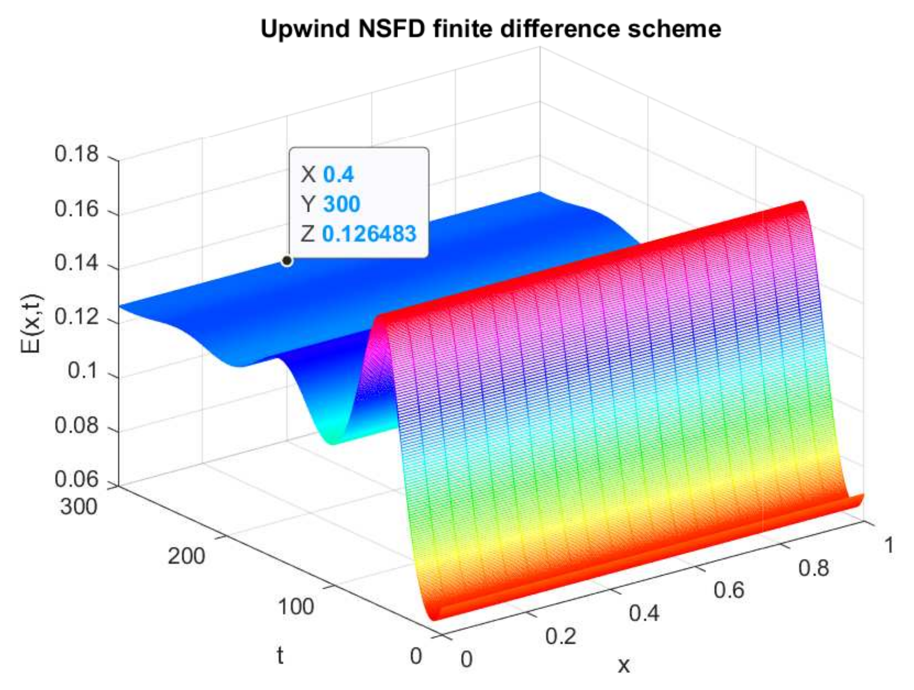
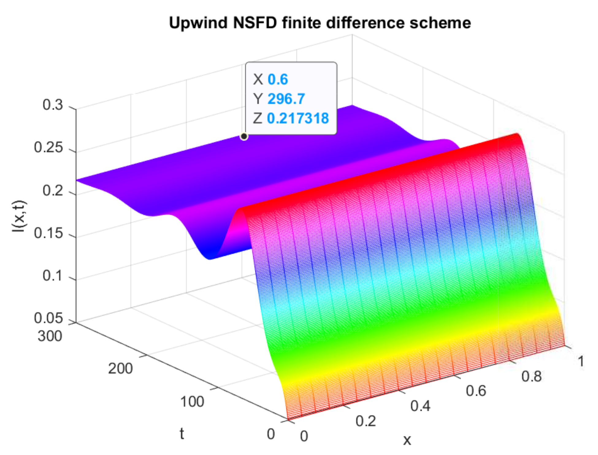
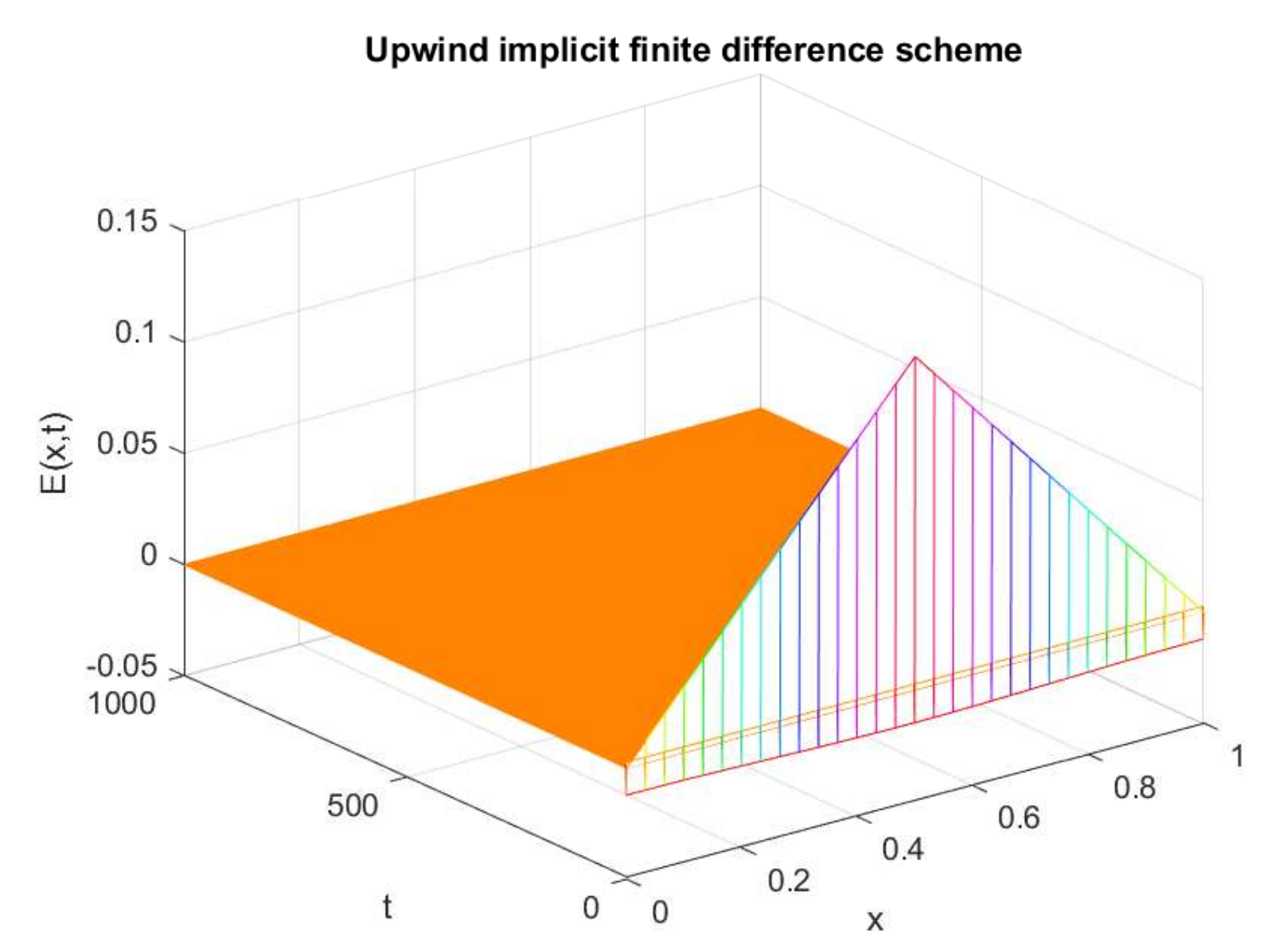
The current study deals with the dynamics of the Ebola virus disease by developing an advective–diffusive nonlinear physical system. The present article elucidates the consequential dynamics of a nonlinear epidemic model of a murderous disease known as the Ebola virus disease. The model of this disease is considered in the generic form; that is, in this model, the advective and diffusive transmission of the virus is kept at a constant rate. The existing epidemic models do not consider the random and directed motions simultaneously in their study. Thus, their studies cannot predict the disease dynamics closely. However, this work seems better for investigating the disease dynamics. Additionally, some widely used schemes in the literature provide negative solutions to the state variables, which are physically meaningless. Therefore, it is a novelty of this scheme that it confirms the positivity as well as the other fundamental traits of the numerical solution. Hence, the developed scheme is a reliable tool to solve the nonlinear epidemic model by taking into account the advection and diffusion situation. This article is composed of two main types of analysis: one is optimal existence analysis and the other is numerical analysis. The results regarding the feasible solutions for the proposed Ebola virus epidemic model are formulated. The analysis regarding the solutions to the considered problem is addressed under some special conditions. The supplementary data (auxiliary data) are also examined. As in the dynamical models, the associated solutions of the model’s equations belong to the set of continuous functions, but it is expedient to look at the particular subsets of the Banach space. A closed subset is considered for the objective optimal values that are explored. The solutions of the model are guaranteed with the help of Schauder’s fixed-point theorem under some feasible constraints. The extension of advection and diffusion terms with constant rates in the equations of the model under study make the study more useful and practical. In the second half of the paper, a numerical analysis is studied. First, the numerical solutions are computed by a well-known nonclassical finite difference template. By adopting the formulas to approximate the derivatives as a function of space and the derivatives as a function of time, a compatible discrete model is designed. It can be observed that the used numerical technique is structure-preserving, which is an important property that should be possessed by the numerical scheme, i.e., the discretized system devised from the numerical template keeps the same features that the associated continuous set of differential equations has retained. We also examined whether a projected formulation is coherent with the planned numerical design. The reliability of the numerical program is validated by applying the Von Neumann condition. Another significant attribute is the non-negativity of the solution variables involved in the model under consideration. Thus, the M-matrix criteria guarantee the positivity of the solutions. Moreover, the assertions are ascertained by some feasible numerical experiments. Numerical simulations of all the considered and proposed schemes are also presented. The simulated graphs depict the various physical features of the relevant scheme. For instance, our scheme provides positive, bounded, and convergent solutions. Thus, all the results reflected by the simulated graphs are in accordance with the pre-assumptions. The results obtained by applying different schemes are also used for comparing the efficacy of the schemes. From the future perspective, this work may be extended to two and three dimensions. The reader should study the physical system by including the advection–diffusion terms in it and construct some structure-preserving numerical schemes for such types of systems.

Author Contributions

Conceptualization, N.S. and N.A.; methodology, T.S.S.; software, N.A. and M.R.; validation, N.A. and A.A.; formal analysis, N.S. and M.A.u.R.; investigation, N.S.; resources, M.D.l.S.; data curation, T.S.S., N.S. and N.A.; writing—original draft preparation, N.S.; writing—review and editing, N.S.; visualization, M.S.I.; supervision, M.A.u.R. and M.S.I.; project administration, N.A. and N.S. All authors have read and agreed to the published version of the manuscript.

Funding

Basque Government, Grants IT1555-22 and KK-2022/00090. MCIN/AEI 269.10.13039/501100011033, Grant PID2021-1235430B-C21/C22.

Data Availability Statement

Not applicable.

Acknowledgments

The authors are grateful to the Basque Government for its support through Grants IT1555-22 and KK-2022/00090 and to MCIN/AEI 269.10.13039/501100011033 for Grant PID2021-1235430B-C21/C22.

Conflicts of Interest

The authors declare no conflict of interest.

References

  1. Dhama, K.; Karthik, K.; Khandia, R.; Chakraborty, S.; Munjal, A.; Latheef, S.K.; Kumar, D.; Ramakrishnan, M.A.; Malik, Y.S.; Singh, R.; et al. Advances in designing and developing vaccines, drugs, and therapies to counter Ebola virus. Front. Immunol. 2018, 9, 1803. [Google Scholar] [CrossRef]
  2. Kourtis, A.P.; Appelgren, K.; Chevalier, M.S.; McElroy, A. Ebola virus disease: Focus on children. Pediatr. Infect. Dis. J. 2015, 34, 893. [Google Scholar] [CrossRef] [PubMed] [Green Version]
  3. Goeijenbier, M.; Van Kampen, J.J.; Reusken, C.B.; Koopmans, M.P.; Van Gorp, E.C. Ebola virus disease: A review on epidemiology, symptoms, treatment and pathogenesis. Neth. J. Med. 2014, 72, 442–448. [Google Scholar] [PubMed]
  4. CDC. Outbreaks Chronology: Ebola Virus Disease. Centers for Disease Control and Prevention (CDC), Atlanta, USA. Available online: Phttps://www.cdc.gov/vhf/ebola/history/chronology.html (accessed on 24 November 2022).
  5. Center for Disease Control and Prevention. Ebola Outbreak in West Africa—Case Counts. 2014. Available online: https://www.cdc.gov/vhf/ebola/history/2014-2016-outbreak/index.html#:~:text=The%20impact%20this%20epidemic%20had,outside%20of%20these%20three%20countries (accessed on 24 November 2022).
  6. World Health Organization. Ebola Virus Disease, Fact Sheet. June 2017. Available online: https://www.who.int/news-room/fact-sheets/detail/ebola-virus-disease (accessed on 24 November 2022).
  7. DRC Ebola Outbreaks: Crisis Update-2019 (Reliefweb). 2 August 2019. Available online: https://reliefweb.int/report/democratic-republic-congo/drc-ebola-outbreaks-crisis-update-2-august-2019 (accessed on 24 November 2022).
  8. Leroy, E.M.; Kumulungui, B.; Pourrut, X.; Rouquet, P.; Hassanin, A.; Yaba, P.; Délicat, A.; Paweska, J.T.; Gonzalez, J.P.; Swanepoel, R. Fruit bats as reservoirs of Ebola virus. Nature 2015, 438, 575–576. [Google Scholar] [CrossRef]
  9. Manguvo, A.; Mafuvadze, B. The impact of traditional and religious practices on the spread of Ebola in West Africa: Time for a strategic shift. Pan Afr. Med. J. 2015, 22 (Suppl. 1), 9. [Google Scholar] [CrossRef]
  10. Feldmann, H.; Sanchez, A.; Geisbert, T. Filoviridae: Marburg and ebola viruses. In Fields Virology, 6th ed.; Wolters Kluwer Health Adis (ESP): Alphen aan den Rijn, The Netherlands, 2013. [Google Scholar]
  11. World Health Organization. Ebola Virus Disease. 2020. Available online: https://www.who.int/news-room/fact-sheets/detail/ebola-virus-disease (accessed on 24 November 2022).
  12. Legrand, J.; Grais, R.F.; Boelle, P.Y.; Valleron, A.J.; Flahault, A. Understanding the dynamics of Ebola epidemics. Epidemiol. Infect. 2007, 135, 610–621. [Google Scholar] [CrossRef] [PubMed]
  13. Althaus, C.L. Estimating the reproduction number of Ebola virus (EBOV) during the 2014 outbreak in West Africa. PLoS Curr. 2014, 6. [Google Scholar] [CrossRef] [Green Version]
  14. Browne, C.; Gulbudak, H.; Webb, G. Modeling contact tracing in outbreaks with application to Ebola. J. Theor. Biol. 2015, 384, 33–49. [Google Scholar] [CrossRef] [PubMed] [Green Version]
  15. Webb, G.F.; Browne, C.J. A model of the Ebola epidemics in West Africa incorporating age of infection. J. Biol. Dyn. 2016, 10, 18–30. [Google Scholar] [CrossRef]
  16. Agusto, F.B. Mathematical model of Ebola transmission dynamics with relapse and reinfection. Math. Biosci. 2017, 283, 48–59. [Google Scholar] [CrossRef] [PubMed]
  17. Bodine, E.N.; Cook, C.; Shorten, M. The potential impact of a prophylactic vaccine for Ebola in Sierra Leone. Math. Biosci. Eng. 2018, 15, 337. [Google Scholar] [CrossRef] [PubMed] [Green Version]
  18. Weitz, J.S.; Dushoff, J. Modeling post-death transmission of Ebola: Challenges for inference and opportunities for control. Sci. Rep. 2015, 5, 8751. [Google Scholar] [CrossRef] [PubMed] [Green Version]
  19. Bonyah, E.; Badu, K.; Asiedu-Addo, S.K. Optimal control application to an Ebola model. Asian Pac. J. Trop. Biomed. 2016, 6, 283–289. [Google Scholar] [CrossRef] [PubMed] [Green Version]
  20. Grigorieva, E.V.; Deignan, P.B.; Khailov, E.N. Optimal control problem for a SEIR type model of ebola epidemics. Rev. MatemáTica Teor. Apl. 2017, 24, 79–96. [Google Scholar] [CrossRef] [Green Version]
  21. Jiang, S.; Wang, K.; Li, C.; Hong, G.; Zhang, X.; Shan, M.; Li, H.; Wang, J. Mathematical models for devising the optimal Ebola virus disease eradication. J. Transl. Med. 2017, 15, 124. [Google Scholar] [CrossRef] [Green Version]
  22. Mhlanga, A. Dynamical analysis and control strategies in modelling Ebola virus disease. Adv. Differ. Equ. 2019, 2019, 458. [Google Scholar] [CrossRef] [Green Version]
  23. Ahmad, M.D.; Usman, M.; Khan, A.; Imran, M. Optimal control analysis of Ebola disease with control strategies of quarantine and vaccination. Infect. Dis. Poverty 2016, 5, 72. [Google Scholar] [CrossRef] [Green Version]
  24. Tulu, T.W.; Tian, B.; Wu, Z. Modeling the effect of quarantine and vaccination on Ebola disease. Adv. Differ. Equ. 2017, 2017, 178. [Google Scholar] [CrossRef] [Green Version]
  25. Area, I.; NdaÏrou, F.; Nieto, J.J.; Silva, C.J.; Torres, D.F. Ebola model and optimal control with vaccination constraints. arXiv 2017, arXiv:1703.01368. [Google Scholar] [CrossRef] [Green Version]
  26. Berge, T.; Lubuma, J.S.; Moremedi, G.M.; Morris, N.; Kondera-Shava, R. A simple mathematical model for Ebola in Africa. J. Biol. Dyn. 2017, 11, 42–74. [Google Scholar] [CrossRef]
  27. Kabli, K.; El Moujaddid, S.; Niri, K.; Tridane, A. Cooperative system analysis of the Ebola virus epidemic model. Infect. Dis. Model. 2018, 3, 145–159. [Google Scholar] [CrossRef]
  28. Rafiq, M.; Ahmad, W.; Abbas, M.; Baleanu, D. A reliable and competitive mathematical analysis of Ebola epidemic model. Adv. Differ. Equ. 2020, 2020, 540. [Google Scholar] [CrossRef]
  29. Okyere, E.; Ankamah, J.D.; Hunkpe, A.K.; Mensah, D. Deterministic epidemic models for ebola infection with time-dependent controls. arXiv 2020, arXiv:1908.07974. [Google Scholar] [CrossRef]
  30. Ahmad, W.; Rafiq, M.; Abbas, M. Mathematical analysis to control the spread of Ebola virus epidemic through voluntary vaccination. Eur. Phys. J. Plus 2020, 135, 775. [Google Scholar] [CrossRef]
  31. Tahir, M.; Inayat Ali Shah, S.; Zaman, G.; Muhammad, S. Ebola virus epidemic disease its modeling and stability analysis required abstain strategies. Cogent Biol. 2018, 4, 1488511. [Google Scholar] [CrossRef]
  32. Dayan, F.; Rafiq, M.; Ahmed, N.; Raza, A.; Ahmad, M.O. A dynamical study of a fuzzy epidemic model of Mosquito-Borne Disease. Comput. Biol. Med. 2022, 148, 105673. [Google Scholar] [CrossRef]
  33. Khan, A.; Zarin, R.; Humphries, U.W.; Akgül, A.; Saeed, A.; Gul, T. Fractional Optimal Control Dynamics of Coronavirus Model with Mittag-Leffler Law. Ecol. Complex. 2021, 45, 100880. [Google Scholar]
  34. Yadava, S.; Kumar, D.; Singh, J.; Baleanu, D. Analysis and Dynamics of Fractional Order COVID-19 Model with Memory Effect. Results Phys. 2021, 24, 104017. [Google Scholar] [CrossRef]
  35. Iqbal, Z.; Macías-Díaz, J.E.; Ahmed, N.; Aziz-ur Rehman, M.; Raza, A.; Rafiq, M. A SEIR model with memory effects for the propagation of Ebola-like infections and its dynamically consistent approximation. Comput. Methods Programs Biomed. 2021, 209, 106322. [Google Scholar] [CrossRef]
  36. Mickens, R.E. Positivity preserving discrete model for the coupled ODE’s modeling glycoly-sis. In Proceedings of the fourth International Conference on Dynamical Systems and Differential Equations, Wilmington, NC, USA, 24–27 May 2002; pp. 623–629. [Google Scholar]
  37. Cantrell, R.S.; Cosner, C. Spatial Ecology via Reaction–Diffusion Equations; Wiley Ser. Math. Comput. Biol.; John Wiley and Sons: Chichester, UK, 2003. [Google Scholar]
  38. Tang, D.; Ma, L. Existence and uniqueness of a Lotka–Volterra reaction–diffusion model with advection term. Appl. Math. Lett. 2018, 86, 83–88. [Google Scholar] [CrossRef]
  39. Boztosuna, I.; Charafi, A. An analysis of the linear advection–diffusion equation using mesh-free and mesh-dependent methods. Eng. Anal. Bound. Elem. 2002, 26, 889–895. [Google Scholar] [CrossRef]
  40. Mojtabi, A.K.; Deville, M. One-Dimensional linear advection–diffusion equation: An-alytical and finite element solutions. Comput. Fluids 2015, 107, 189–195. [Google Scholar] [CrossRef] [Green Version]
  41. Ervin, V.J.; Macías-Díaz, J.E.; Ruiz-Ramírez, J. A positive and bounded finite element approximation of the generalized Burgers–Huxley equation. J. Math. Anal. Appl. 2015, 424, 1143–1160. [Google Scholar]
  42. WHO (World Health Organization). Ebola Data and Statistics. Available online: http://apps.who.int/gho/data/view.ebola-sitrep.ebola-country-LBR (accessed on 24 November 2022).
  43. Rachah, A.; Torres, D.F.M. Dynamics and Optimal Control of Ebola Transmission. Math. Comput. Sci. 2016, 10, 331–342. [Google Scholar] [CrossRef] [Green Version]
  44. Rachah, A.; Torres, D.F.M. Mathematical modelling, simulation and optimal control of the 2014 Ebola outbreak inWest Africa. Discret. Dyn. Nat. Soc. 2015, 2015, 842792. [Google Scholar]
  45. IndexMundi. Available online: http://www.indexmundi.com (accessed on 24 November 2022).
  46. Durojaye, M.; Ajie, I.J. Mathematical Model of the Spread and Control of Ebola Virus Disease. Appl. Math. 2017, 7, 23–31. [Google Scholar] [CrossRef]
  47. Fujimoto, T.; Ranade, R. Two characterizations of inverse–positive matrices: The Hawkins–Simon condition and the Le Chatelier—Braun principle. Electron. J. Linear Algebra 2004, 11, 59–65. [Google Scholar] [CrossRef]
Figure 1. Numerical solution of S ( x , t ) (susceptible individuals) by employing upwind NSFD technique at endemic equilibrium point with p 0 = 0.03507 , p 1 = 0.0099 , p 2 = 0.2 , p 3 = 0.1887 , p 4 = 0.1 .
Axioms 12 00079 g001
Figure 2. Numerical solution of E ( x , t ) (exposed individuals) by employing upwind NSFD technique at disease-free point with p 0 = 0.03507 , p 1 = 0.0099 , p 2 = 0.2 , p 3 = 0.1887 , p 4 = 0.1 .
Axioms 12 00079 g002
Figure 3. Numerical solution of I ( x , t ) (infected individuals) by employing upwind NSFD technique at disease-free point with p 0 = 0.03507 , p 1 = 0.0099 , p 2 = 0.2 , p 3 = 0.1887 , p 4 = 0.1 .
Axioms 12 00079 g003
Figure 4. Numerical solution of S ( x , t ) , E ( x , t ) , and I ( x , t ) by employing upwind NSFD technique at disease-free point with p 0 = 0.03507 , p 1 = 0.0099 , p 2 = 0.2 , p 3 = 0.1887 , p 4 = 0.1 .
Axioms 12 00079 g004
Figure 5. Numerical solution of S ( x , t ) (susceptible individuals) by employing upwind NSFD technique at disease-free point with λ 1 = λ 2 = λ 3 = 0.8 and μ 1 = μ 2 = μ 3 = 0.02 .
Axioms 12 00079 g005
Figure 6. Numerical solution of E ( x , t ) (exposed individuals) by employing upwind NSFD technique at disease-free point with λ 1 = λ 2 = λ 3 = 0.8 and μ 1 = μ 2 = μ 3 = 0.02 .
Axioms 12 00079 g006
Figure 7. Numerical solution of I ( x , t ) (infected individuals) by employing upwind NSFD technique at disease-free points with λ 1 = λ 2 = λ 3 = 0.8 and μ 1 = μ 2 = μ 3 = 0.02 .
Axioms 12 00079 g007
Figure 8. Numerical behavior of all subpopulations by employing upwind NSFD technique at disease-free point with x = 1 , λ 1 = λ 2 = λ 3 = 0.8 and μ 1 = μ 2 = μ 3 = 0.02 .
Axioms 12 00079 g008
Figure 9. Numerical solution of S ( x , t ) (susceptible individuals) by employing the proposed scheme at endemic point with λ 1 = λ 2 = λ 3 = 0.8 and μ 1 = μ 2 = μ 3 = 0.02 .
Axioms 12 00079 g009
Figure 10. Numerical solution of E ( x , t ) (exposed individuals) by employing the proposed scheme at an endemic point with λ 1 = λ 2 = λ 3 = 0.8 and μ 1 = μ 2 = μ 3 = 0.02 .
Axioms 12 00079 g010
Figure 11. Numerical solution of I ( x , t ) (infected individuals) by employing the proposed scheme at an endemic point with λ 1 = λ 2 = λ 3 = 0.8 and μ 1 = μ 2 = μ 3 = 0.02 .
Axioms 12 00079 g011
Figure 12. Numerical behavior of all subpopulations by employing upwind NSFD technique at an endemic point with x = 1 , λ 1 = λ 2 = λ 3 = 0.8 and μ 1 = μ 2 = μ 3 = 0.02 .
Axioms 12 00079 g012
Figure 13. Numerical solution of E ( x , t ) (exposed individuals) by employing Crank–Nicolson technique at disease-free point with λ 1 = λ 2 = λ 3 = 0.16 and μ 1 = μ 2 = μ 3 = 64 .
Axioms 12 00079 g013
Figure 14. Numerical solution of E ( x , t ) (exposed individuals) by employing Crank–Nicolson technique at endemic point with λ 1 = λ 2 = λ 3 = 0.16 and μ 1 = μ 2 = μ 3 = 64 .
Axioms 12 00079 g014
Figure 15. Numerical solution of E ( x , t ) (exposed individuals) by employing upwind NSFD technique at disease-free point with λ 1 = λ 2 = λ 3 = 0.16 and μ 1 = μ 2 = μ 3 = 64 .
Axioms 12 00079 g015
Figure 16. Numerical behavior of E ( x , t ) (infected individuals) by employing upwind NSFD technique at endemic point with λ 1 = λ 2 = λ 3 = 0.16 and μ 1 = μ 2 = μ 3 = 64 .
Axioms 12 00079 g016
Figure 17. Numerical solution of E ( x , t ) (exposed individuals) by employing upwind implicit technique at disease-free point with λ 1 = λ 2 = λ 3 = 0.3 and μ 1 = μ 2 = μ 3 = 180 .
Axioms 12 00079 g017
Figure 18. Numerical solution of E ( x , t ) (exposed individuals) by employing NSFD technique at disease-free point with λ 1 = λ 2 = λ 3 = 0.3 and μ 1 = μ 2 = μ 3 = 180 .
Axioms 12 00079 g018
Table 1. Values of the parameters.
NotationsDescription
S ( x , t ) No. of susceptible individuals at time t and space x
E ( x , t ) No. of exposed individuals at time t and space x
I ( x , t ) No. of infected individuals at time t and space x
R ( x , t ) No. of recovered individuals at time t and space x
p 1 Birth rate as well as death rate
p 2 Contact rate for the individuals from the susceptible with infected class
p 3 Transmission rate of exposed persons to the infected person
p 4 Treatment rate
a 1 Rate of advection for the susceptible class
a 2 Rate of advection for the exposed class
a 3 Rate of advection for the infected class
a 4 Rate of advection for the recovered class
δ 1 Diffusion rate of advection for the susceptible class
δ 2 Diffusion rate of advection for the exposed class
δ 3 Diffusion rate of advection for the infected class
δ 4 Diffusion rate of advection for the recovered class
Disclaimer/Publisher’s Note: The statements, opinions and data contained in all publications are solely those of the individual author(s) and contributor(s) and not of MDPI and/or the editor(s). MDPI and/or the editor(s) disclaim responsibility for any injury to people or property resulting from any ideas, methods, instructions or products referred to in the content.

