1. Introduction
In [
1], S. N. Bernstein constructed positive and linear operators (named after him) as Bernstein operators to prove the famous Weierstrass approximation theorem. The Bernstein operators attached to
ℑ:
(the space of continuous functions on
S endowed with the max-norm
)
with
were defined by
where
,
,
. Later, many generalizations and modifications of these kinds of operators (
1) have been constructed and considered, we refer the readers to these papers (see
-Bernstein operators [
2], generalized Bernstein operators [
3,
4], blending-type Bernstein operators [
5,
6,
7], Durrmeyer-type Bernstein operators [
8], genuine-type Bernstein operators [
9,
10], and so on).
In [
11], F. Usta constructed a new modification of Bernstein operators attached to
ℑ:
by means of the second-order central moments of the Bernstein operators (
1) as:
where
In [
12], Y. S. Wu et al. defined
q-generalization of operators (
2). In [
13], Q. B. Cai et al. developed a Beta-type modification of operators (
2). Recently, many generalizations and modifications of operators (
2) were introduced and studied, we refer the readers to the articles [
14,
15]. Motivated by the above works, for
, we present the blending-type modified Bernstein–Durrmeyer operators involving a strictly positive function
and
as follows:
where
,
and Beta function
,
.
If we take
, then we obtain the operators defined in [
13]. If we take
, then we obtain the operators defined in [
14].
In the rest part of the paper, we investigate the approximation properties of the operators
. In
Section 2, we yield the calculation formulas for the moment and central moment related to the operators
. In
Section 3, we yield an asymptotic formula for operators (
3). In
Section 4 and
Section 5, we establish the local and global approximation theorems by using the classical modulus of continuity and
K–functional. In
Section 6, we derive the rate of convergence for functions with a derivative of bounded variation. In
Section 7, we make the concluding remarks on our works. We show the advantage of the operators
by some numerical experiments.
2. Auxiliary Lemmas
In this section, we establish several lemmas to prove our main approximation properties for operators (
3). Let
,
be the test functions, which play a key role in the study of the approximation properties of the positive linear operators.
Lemma 1. ([12], Lemma 1 and Lemma 2, q = 1) Let , , and . Then, the following relations hold: By using direct calculation, we obtain the following three lemmas.
Lemma 2. Let , , and , . We conclude Lemma 3. Let , , and . We conclude Lemma 4. For and , we conclude Lemma 5. Let , and fix . Then, holds uniformly on S.
Proof. Note that
,
,
as
hold uniformly on
S. Applying the classic Korovkin Theorem in [
16], it follows that
holds uniformly on
S. □
Lemma 6. Let , , and fix . Then, we have .
Proof. Using the definition of the operators
and taking Lemma 2 into account, it follows
□
4. Local Approximation
In this section, we study the local approximation properties for the newly defined operators
in terms of the modulus of continuity, Peetre’s
K-functional, the Steklov mean function and the elements of Lipschitz function class. For
, the classical modulus
and the second-order modulus
of
ℑ are defined respectively by:
The Peetre’s
K-functional is given by
It is known from [
16] that
where
is a constant depending only on
ℑ.
For
and
, the Steklov mean function is defined by
From direct calculation, we have (i) .
(ii) and .
In [
17], Lenze introduced the following Lipschitz-type maximal function of order
for a function
as
In [
18], M. A. Özarslan and H. Aktuğlu defined the following Lipschitz-type space involving two parameters
as
where
and
is a positive constant depending at most on
and
.
Now, we prove the following theorems on the local approximation properties of operators (
3).
Theorem 2. Let , , , and . We have Proof. By using the property of
, we derive
Combining the linearity and the monotonicity of operators (
3), we have
Choosing , we get the desired result. □
Theorem 3. Let , , , and . We have Proof. For any
, we have
Applying the operators
on both sides of the above equality, we can write
By using the property of
, we derive
Hence, by using the Cauchy–Buniakowsky–Schwarz inequality, we have
Now, choosing , we get the desired inequality. □
Theorem 4. Let , , , and . Then, there exists a constant such that for any where . Proof. For any
and
, we construct the auxiliary operators as follows:
Then, we can easily check that
For any
and
, by using Taylor’s expansion formula, we have
Applying the operators
on both sides of the above equality, we can write
In view of (
12) and Lemma 6, we obtain
Furthermore, using the definition (
12) of the operators
and (
13), we obtain that
Taking the infimum on the right-hand side over all
and combining inequality (
10), we have
Then, the proof of Theorem 4 is completed. □
Theorem 5. Let , , , and . Then, we have Proof. For
, using the definition of the Steklov mean, we obtain
Using property (i) of the Steklov mean and Lemma 6, we obtain
It follows from Taylor’s expansion formula that
Again using property (i) of the Steklov mean and Lemma 6, we get
Choosing , the proof of Theorem 5 is completed. □
Theorem 6. Let . If , then we have Proof. We first deal with the case
. We obtain
Using the fact that
and the Cauchy–Buniakowsky–Schwarz inequality, we have
Thus, the inequality is obtained for
. Next, we prove the inequality for the case
. Applying the Hölder’s inequality with
and
, we get
Hence, the desired result is obtained. □
Theorem 7. Let and . Then, for all , we have Proof. Applying the Hölder’s inequality with
and
, we obtain
□
5. Global Approximation
In this section, we yield a theorem on the global approximation properties of operators (
3) by using the weighted first- and second-order modulus of smoothness. Let us define the space of functions
, where
means that
is differentiable and
is absolutely continuous on every closed interval
. Let
and
. The weighted
K-functional is defined by
The weighted first- and second-order modulus of smoothness are defined by
and
where
and
ℓ above are admissible step-weight functions defined on
S. By [
19], there exists a constant
, such that
Our next result is the following theorem.
Theorem 8. Let , , , and . Thenwhere , , and is a constant. Proof. Again, considering the auxiliary operators defined at (
12) and for
, applying the operators
on both sides of the inequality mentioned above, we have
Since
is concave function on
S, taking
, with
and
, we have
On the other hand, we observe that
Combining (
16)–(
18), we have
Applying the definition of
in this section, we find
Further, for
, since the operators
are uniformly bounded, using the above inequality, we have
Taking infimum over all
, we get
As for the last part above, we find
Combining (
19) with the above results, we complete the proof of Theorem 8. □
6. Rate of Convergence
The goal of this section is to study the convergence rate of
for functions with a derivative of bounded variation on
S. Let
denote the class of absolutely continuous functions defined on
, whose derivatives have bounded variation on
. It is well known that the functions
possess a representation:
where
is a function with bounded variation on
. An integral representation of the operators
can be given as follows:
where the kernel
.
Lemma 7. For a sufficiently large λ and a fixed , we have
- (a)
- (b)
.
Proof. We prove (a) as follows.
The proof of (b) is similar to that of (a). We omit the details. □
Theorem 9. Let . Then, for every and sufficiently large λ, the following inequalityholds, where is the total variation of on and is defined by Proof. Since
, by (
20), for each
, we get
On the other hand, for any
, by (
21), we decompose
as follows
where
From (
20), we have
meanwhile, we have
Using Lemma 3 and considering (
22)–(
25), we obtain
Thus, our task is to estimate the terms and .
From the definition of
, we write
Since the inequality
holds for any
, applying the integration by parts with putting
, we obtain
By considering
, we yield
Again, applying integration by parts to
, together with Lemma 7, we have
By the substitution of the values
, we get
Collecting the estimates (
26)–(
28), we get the desired results. Hence, the proof of Theorem 9 is completed. □
7. Conclusions
In our paper, we construct the blending-type modified Bernstein–Durrmeyer operators involving the strictly positive function and the positive parameter . We derive many approximation properties of this type of operator. We first establish a Voronovskaya-type asymptotic theorem of them. Then, we establish the local and global approximation theorems by using the classical modulus of continuity and K-functional. Finally, we derive the convergence rate of the approximation for functions with a derivative of bounded variation.
We remark that our results are rather general. For instance, one can get the error estimates from our results for different existing Bernstein–Durrmeyer–type operators, such as operators given in [
14,
15], by selecting different parameters
and
. Moreover, we can obtain the new operators, which provide better approximations for different target functions. In general, different target functions need different parameters. The choices of the parameters show the flexibility of the operators
. In fact, for a given target function
ℑ, we can choose appropriate parameters to obtain a smaller error of the approximation by
. This feature will be of great interest to practical applications. We illustrate this feature by some numerical experiments.
Example 1. Let , , , and .
Figure 1 shows the convergence of the operators
to the target function
while we choose different parameters
. The larger the
, the smaller of the error of the approximation by
. Combining with
Figure 2, when
, the error of the approximation
becomes smaller and smaller with the increase of variable
. When
, contrary to what happens.
It is known that if we take
in operators (
3), then we get the modified Bernstein–Durrmeyer-type operators
, which is defined in [
14]. In the following example, we show that operators (
3) with some different parameters provide better approximations than the operators
.
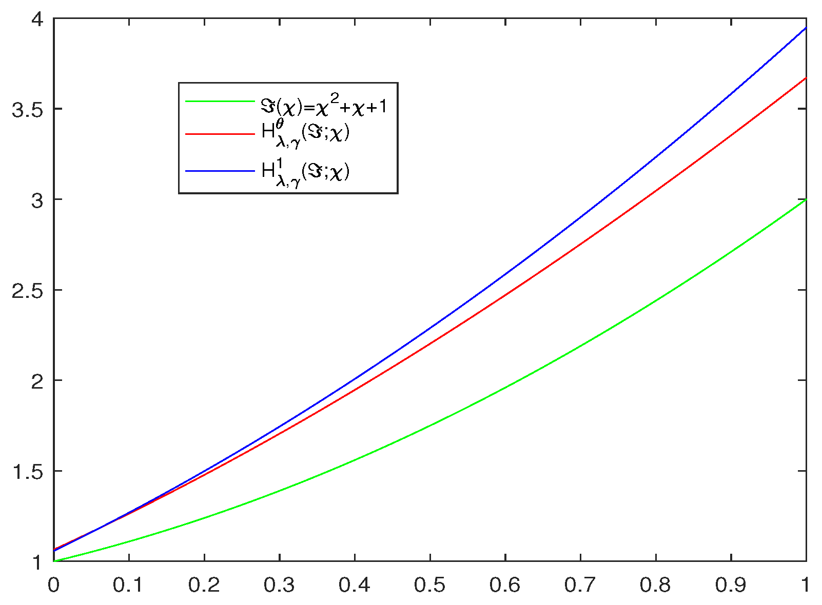
Example 2. Let , , , and .
From
Figure 3, we can see that, for the target function
(green), the operator
(red) gives a better approximation to
than the modified Bernstein–Durrmeyer type operator
(blue).


