Object-Based Dynamics: Applying Forman–Ricci Flow on a Multigraph to Assess the Impact of an Object on The Network Structure

Abstract

Temporal information plays a central role in shaping the structure of a network. In this paper, we consider the impact of an object on network structure over time. More specifically, we use a novel object-based dynamic measure to reflect the extent to which an object that is represented in the network by a vertex affects the topology of the network over time. By way of multigraph and Forman–Ricci flow, we assess the object’s impact on graph weights by comparing two graphs, one in which the object is present and one in which the object is absent. After using a case study to demonstrate the impact of Forman–Ricci flow on the network structure, we apply our measure in a semantic network to assess the effects of a word on the interactions between other words that follow it. In addition, we compare our novel measure to centrality and curvature measures so that we can ascertain the advantages of our measure over ones that already exist.

1. Introduction

Complex network theory provides a useful way to represent complex relationships among different objects; previous research has focused on social, genetic, neurological, psychopathological, economic, and semantic contexts [1,2,3,4,5,6]. The structural elements are, first, a set of vertices within the network, representing elements such as individuals, genes, or words, and second, a set of edges representing the interaction between those vertices. This paper focuses on directed and weighted networks, in other words, networks in which interactions may occur in a specific direction and with a certain strength.

One of the basic assumptions in many studies involving complex networks is that static networks can model real-world phenomena. The problem with this assumption is that real-world interactions, such as social or economic transactions, evolve. The network, then, must be dynamic, with a temporal dimension that captures information about the changing interactions between objects. Dynamical network analysis such as temporal network [7] or stream graph [8] amplifies the temporal dimension in the analysis. A temporal network captures changes in the interactions between vertices as well as the appearance and disappearance of vertices.

In a dynamical evolution, one can investigate differences between networks [9] or take a dynamical approach to community detection [10]. Our own aim is to detect the extent to which an object changes the network’s structure over time, and we include here the effect on the neighborhood of the interaction, too. In other words, we want to see how an object changes not only the interaction between a pair of objects but also the larger environment that surrounds that interaction.

In a social setting, for instance, the presence of a specific individual may change the way other individuals interact; in the language of a network, the individual affects the set of vertices in the environment of the interaction. In a commercial context, the purchase of product A may affect the rest of the buying process, leading to the purchase of products B and C together. Without the purchase of A, B and C might not have been purchased at the same time.

In this paper, we harness tools from differential geometry and complex networks to investigate the interplay between an object and the dynamics of network structure. We offer a novel measure, the object-based dynamic measure, to account for how an object changes the network topology and the interactions between other objects over time. Our measure is based on two essential elements. First is a multigraph representation for each object. In this multigraph, any pair of vertices receives two sets of edges. One set expresses the interaction between the vertices in the absence of the object, and the other set expresses the interactions in the presence of the object. This multigraph representation allows us to compare the set of interactions with and without the presence of a given object. The second element of our measure is the computation of Ricci flow as a regularization term for each set of edges separately. Ricci flow allows us to extract the geometrical information that reflects the core structure of the network [11,12]. By comparing metrics of the same size for both sets of edges—in other words, the metric both with and without the presence of the object—we can assess the influence of that object on the core geometry of the network.

Our object-based dynamic measure can be used in two ways. The first option takes into account the direction of the effect. As we will explain later, when a negative value represents an object that changes the metric, the structure is tree-like, and when a positive value represents an object that changes the metric, the structure is spherical. The second option takes into account the absolute value of the object-based dynamic, which represents the extent that an object changes the metric. In this case, we know only that a significant change has occurred, not whether the structure is tree-like or spherical. This study presents both options.

After presenting the measure and its essential elements, we present the case study of a semantic network. We apply our object-based dynamic perspective to an ongoing semantic retrieval task so that we can assess a word’s impact, if any, on the semantic interactions that follow that word. More specifically, we examine a graph that represents a standard semantic task: the participants’ production, over the course of one minute, of as many unique words as possible within a semantic category, such as animals. In this context, we can assess the impact of a specific word on the interactions that follow. In the stream of associations, sun-fire-sphere, for example, the word “sun” affects the semantic relationship between “fire” and “sphere.” In the presence of “sun”, “fire” and “sphere” are closely related, but in the absence of “sun,” the relationship between those two words would be weaker.

The purpose of our semantic case study is threefold. First, we want to demonstrate the effect of Ricci-flow as a regularization term on the network structure. Following the studies of Weber, Jost, and Saucan [11] and Ni, Lin, Luo, and Gao [13], which examined different uses of Olivier-Ricci flow and Forman–Ricci flow, we propose a comparison of Forman–Ricci flow between two graphs as a way to examine the impact of an object on the graph weights. Second, we are interested in the results when we apply the measure in a semantic context: we want to examine the extent to which a word affects the interactions between other words that follow it. Third, we want to demonstrate that the object-based dynamic score is not a graph measure but a comparison between two graphs for each object.

This third goal notwithstanding, we compare our novel measure to the centrality measures of degree, closeness, betweenness, LDC, and PageRank. This focus on centrality measures makes sense because a vertex that controls the flow of information is likely to affect the relationship between other vertices over time. We also compare our object-based dynamic to the curvature-based measures Menger, 1-dimensional Forman, 2-dimensional Forman, and Haantjes since these measures provide insight into the local geometric properties near the vertex as well as the topological structure of the network [14,15,16,17]. Finally, we compare our object-based dynamic to the psycholinguistic measures of word frequency and word location since both of these measures reflect attributes of words that may express local changes in the environment of a given word [18]. Through these comparisons, we investigate whether our word-based dynamic measure contributes information beyond what is already provided by centrality, curvature-based, and psycholinguistic measures. We aim to show that the effect of a word on its environment, as measured by our object-based dynamic, is not captured by existing measures.

This paper makes three major contributions: a new perspective in the analysis of network dynamics, with a focus on the effect of an object on network structure; a novel object-based dynamic measure; and the application of this perspective and measure to a semantic graph.

The remainder of this paper is organized as follows. Section 2 presents the data we use in our semantic study case, along with some basic assumptions. Section 3 presents our results with reference to Forman–Ricci flow and our object-based dynamic measure, along with a comparison between our measure and others that already exist. Finally, we present our conclusions in Section 4.

2. Materials and Methods

The experiment was conducted on two groups (N = 2047), both consisting of native Hebrew speakers. One group was recruited from the Hebrew University of Jerusalem (HUJI: N = 691; M:F = 1:1.002; mean age = 24.6 years; range: 18–39); the members of this group received coupons for coffee. The second group (P4A: N = 1356; M:F = 1:1.96; mean age = 29.07 years; range: 18–40) was recruited through the website www.panel4all.co.il (accessed on 15 September 2022), and participants were compensated with gift certificates from the panel4all organization. The ethics committee of the Department of Psychology at the Hebrew University of Jerusalem approved all experimental procedures.

Participants were given one minute in a category fluency test (CFT); the task was to produce as many unique words as possible within the semantic category of animal names. Participants from HUJI were recorded on a Philips DVT4010, and soundtracks were transcribed with the PRAAT program [19], which gave us the words as well as the time signatures for the beginning and end of each word. Participants from P4A were recorded on a phone application, and these soundtracks, too, were transcribed via PRAAT.

Two lists were generated for each participant: a list of words and a list of timestamps, with each timestamp indicating the start time of the word’s retrieval. The timestamps started at 0, indicating the beginning of the recording, and ended at 60.

We begin by describing the manner in which we construct the semantic graph. Let $G=\left(V,E,w\right)$ be an edge-weighted and directed graph, with $V=\left\{v_1,v_2\dots v_n\right\}$ a set of vertices and $E=\left\{\left(v_i,v_j\right)\right\}$ a set of edges or links between words $v_i$ and $v_j$ in V. The words are the vertices, and the edges reflect the relationship between words. The weight $w_{ij}$ was based on the assumption that the closer the semantic relationship between two words, the faster the transition between these two words [20]. The weights of the edges were based on a proposal by Nachshon, Cohen, and Maril [21] and were calculated by a “distance” function that assumes, as expected for a metric, that the “distance” is non-negative. We did not assume symmetry, and we also allowed violations of the triangle inequality. Our “distances,” therefore, did not constitute a true metric.

Our “distance” function calculates the weights of the edges as follows. For any ordered pair of vertices $v_i,v_j$, p = p(s) is a sublist of participant s; the sublist starts at $v_i$ and ends at $v_j$ and denotes the amount of normalized time that it took s to traverse from $v_i$ to $v_j$. Here, each timestamp was normalized by the number of words that s produced. The “distance” function has two free variables that determine the upper and lower boundaries, WS (window size) and MS (minimum subjects):

1.

The upper boundary window size (WS) defines the maximum number of words between $v_i \mathrm{and} v_j$. The sublist p is therefore taken into account when the number of words between $v_i$ and $v_j$ is less than or equal to the number WS.

2.

MS is a number defining the lower boundary, which is the minimum number of p’s containing $v_i$ and $v_j$ in that order, and with, at most, WS words between them.

Let P be the set of the amount of time it took any p to traverse from $v_i$ to $v_j$ up to WS words. The distance between the ordered pair $v_i$ and $v_j$ is then defined as the median of the set P, if |P| > MS. Otherwise, there will be no distance between $v_i$ and $v_j$. In other words, a distance is well-defined iff |P| > MS. The length of any path on the graph will be the sum of the weights (or distances) of the edges composing it, as defined above. Additionally, $d_{ij}$ denotes the shortest path, given by Dijkstra’s shortest path algorithm, from $v_{\mathrm{i}}$ to $v_{\mathrm{j}}$ based on $w_{ij}$.

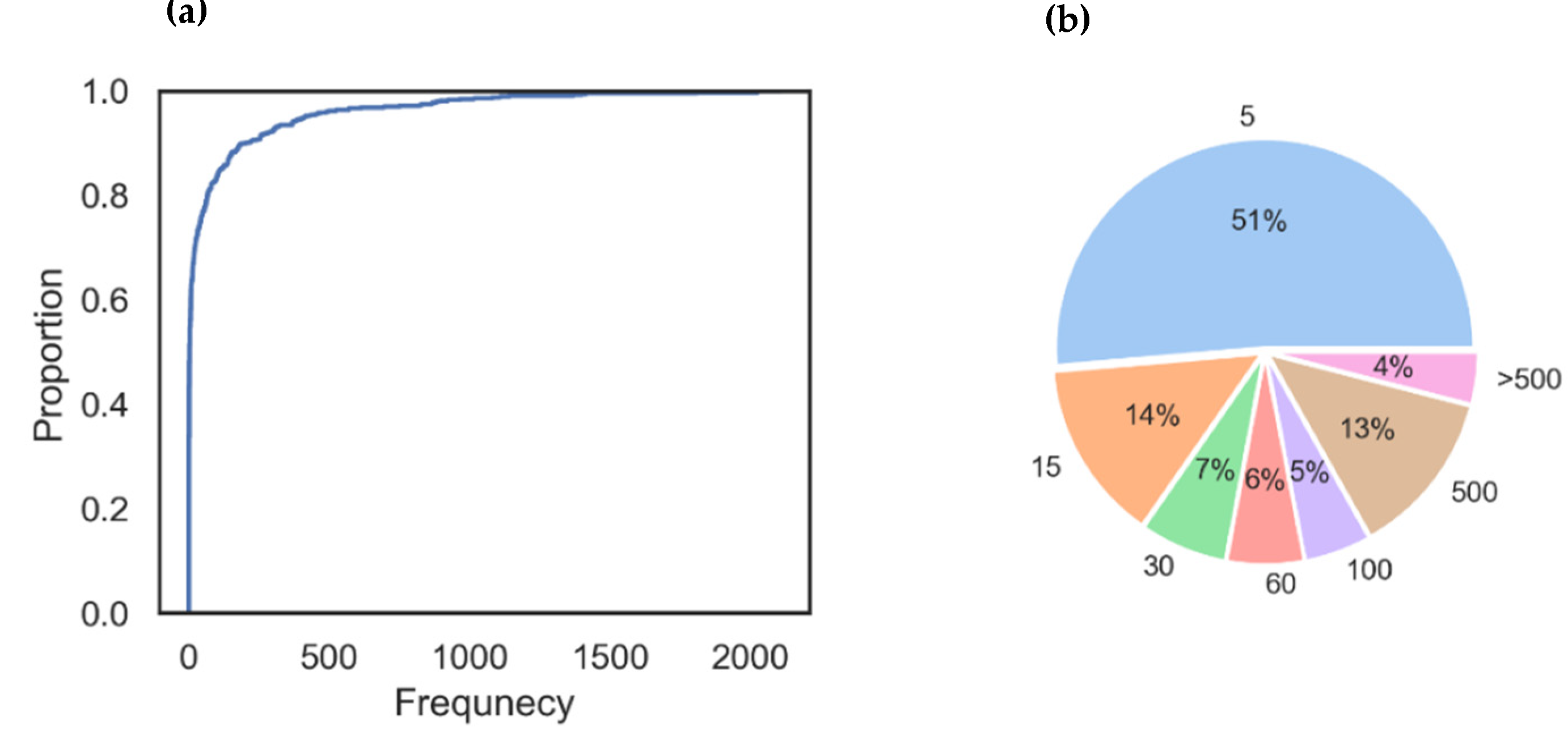
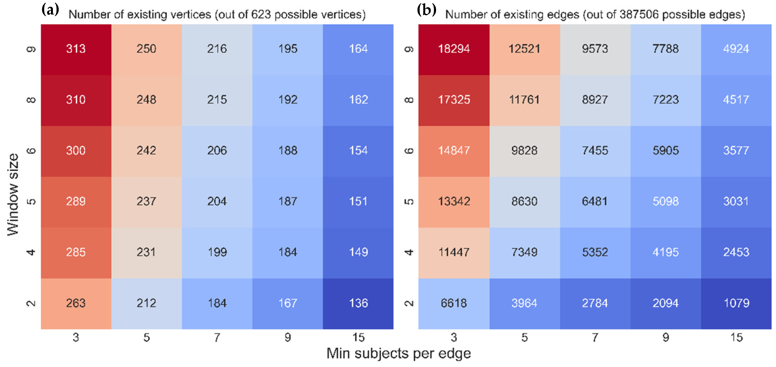
By aggregating temporal information into a pre-defined window size, WS enables us to collapse temporal information into a snapshot static network. The greater the window size, the more fully the snapshot summarizes the broader temporal information. As a result, manipulation of window size allows us to compare snapshots with different degrees of temporary resolution. Descriptive analyses, such as the number of vertices with edges as a function of the free parameters WS and MS, are presented in Appendix A.

3. Results

This part of our paper is divided into three subsections. In Section 3.1, we focus on Forman–Ricci flow, the geometric tool that we use in our object-based dynamic measure, and offer an empirical demonstration of its effect on network structure. In Section 3.2, we present our novel measure and demonstrate how it can be used in a semantic context to quantify the impact of a word on the interactions between the words that follow. Section 3.3 compares our measure with centralities, scalar Ricci-curvature, frequency, and word location.

3.1. Forman–Ricci Flow

Our object-based dynamic measure relies on the notion of Forman–Ricci flow. In this subsection, we introduce Forman–Ricci curvature and then explain Forman–Ricci flow. We then present several analyses that demonstrate the impact of Forman–Ricci flow on the graph weights.

3.1.1. Forman–Ricci Curvature

In Riemannian geometry, the sectional curvature of a tangent plane captures, among other things, the dispersion of geodesics. Three basic behaviors can be distinguished for two geodesics with the “same” velocity and starting point. If they move away exponentially, the result is negative curvature (hyperbolic space). If they move away linearly, the result is zero curvature (Euclidean space). Finally, if they move away logarithmically, the result is positive curvature (spherical space). Ricci curvature of a given geodesic c generalizes the dispersion of geodesics in all the planes to which c belongs. In other words, Ricci curvature, which is defined on smooth manifolds, measures the degree to which the manifold deviates from being locally Euclidean in various tangential directions. Ricci curvature, therefore, carries information about a given geodesic’s local environment. In the discrete case, Ricci curvature is an edge measure that describes how well the neighborhood of the edge is connected; the measure, therefore, provides information not only on edge but also on the neighborhood of an edge.

Here, we focus on Forman–Ricci curvature. Forman [22] introduced a discrete notion of Ricci curvature based on the Bochner–Weitzenböck formula, which preserves the notion of the dispersion of geodesics in a discrete setting [23]. Forman defined a discrete notion of Ricci curvature for general geometric objects, the so-called weighted CW complexes. For our purposes, it is sufficient to introduce Ricci curvature for the limiting case of 1-dimensional simplicial complexes [24], i.e., graphs. For a directed and weighted graph, we use the 1-dimensional Forman–Ricci curvature (FR1) formulated by Saucan, Sreejith, Vivek-Ananth, Jost, and Samal [16]. In this version, three variables determine whether and to what degree FR1 is positive or negative. The key attributes for estimating the Ricci-curvature for edge e = $(v_1,v_2$) in a directed and weighted graph are the following:

1.

The smaller the weight $w_e$ of the edge $e$, the more positive the curvature of $e$.

2.

The greater the weighted in/out-degree of $v_1$ and $v_1$, the more positive the curvature of $e$. The weighted in-degree of vertex $v_1$ takes into account the weights $e_{1j}$, where $e_{1j}=\left(v_{1, }{v}_j\right), j\ne 2$, while the weighted out-degree of vertex $v_2$ takes into account the weights $e_{j2},$ where $e_{j2}=\left(v_{j, }{v}_2\right), j\ne 1$.

3.

The smaller the $\mathrm{deg}(v_1)$ and/or $\mathrm{deg}(v_2)$, the more positive the curvature of $e$.

Forman–Ricci curvature $FR1\left(e\right)$ in a directed and weighted graph is given by the following formula:

$$FR1\left(e\right)=w_e\left(\frac{w_{v_1}}{w_e}- {\displaystyle \sum }_{e_{I,v_1}~e}\frac{w_{v_1}}{\sqrt{w_e{w}_{e_{I,v_1}}}}\right)+ w_e\left(\frac{w_{v_2}}{w_e}- {\displaystyle \sum }_{e_{O,v_2}~e}\frac{w_{v_2}}{\sqrt{w_e{w}_{e_{O,v_2}}}}\right)$$

(1)

where $e$ denotes the edge between vertices $v_1$ and $v_2$, $w_e$ denotes the weight of the edge $e$, and $w_{v_1}$ and $w_{v_2}$ denote the weights associated with vertices $v_1$ and $v_2$. We define $w_{v_i}=1$, $i=1, 2$ (In Forman’s formula (1) it is possible to take into account the weights of the vertices $w_{v_1}$ and $w_{v_2}$. However, in this framework, we used the minimal necessary assumptions, and we, therefore, defined the weights of the vertices as 1. Further research may take up different definitions of the vertices’ weights). In addition, let $e_{I,v_1}~e$ denote the incoming edges incident on vertex $v_1$ and $e_{O,v_2}~e$ denote the outgoing edges emanating from vertex $v_2$. The scalar $FR1$ curvature of vertex v in a graph is defined as follows:

$$FR1\left(v\right)={\displaystyle \sum }_{T_e~ v}FR1\left(e\right)$$

(2)

To clarify the link between Forman–Ricci curvature and the dispersion of geodesics, let us examine that link on an undirected and combinatorial graph, in other words, a 1-dimensional complex with only 0-simplices (vertices) and 1-simplices (edges). In this case, all weights—both edge and vertex ones—equal 1; therefore, Formula (1) simplifies as follows:

$$FR1\left(e\right)=4-\mathrm{deg}\left(v_1\right)-\mathrm{deg}\left(v_2\right)$$

(3)

Thus, in this simple case, only the number of the edges incident to $e$, affects the magnitude of Forman–Ricci curvature. In consequence, the larger the number of the edges incident to $e$, the more negative the curvature, hence the information that passes through $e$ disperses to other vertices. In other words, given that in Formula (3), the number of edges incident to $e$ is determined only by the degree of vertices—the smaller the number of edges incident to $e$, the less dispersed the information passing through $e$.

3.1.2. Forman–Ricci Flow

Hamilton [25] introduced the notion of Ricci flow to reflect how the metric deforms a Riemannian manifold and to smooth out irregularities in the metric. More precisely, Ricci flow changes the metric such that regions with negative Ricci curvature expand and regions with positive Ricci curvature shrink.

In a discrete setting, a combinatorial version was introduced by Chow and Luo [26]. As in the continuous case, Ricci flow processes expand edges with highly negative Ricci curvature and shrink edges with highly positive Ricci curvature. The present article relies on the work of Weber, Jost, and Saucan [11], which applied Forman–Ricci flow for anomaly detection in the network, as well as the work of Ni, Lin, Luo, and Gao [13], which applied Ollivier–Ricci flow to reveal the community structure of a network and demonstrated that the removal of edges with high weights enables the detection of communities in the network.

Following the work of these researchers, for each iteration t, we define Ricci flow as follows:

$$w_{ij}^{t+1}=d_{ij}^t-\left(\eta \cdot {\kappa }_{ij}^t\cdot d_{ij}^t\right) ,$$

(4)

where $\eta$ is the learning rate of the gradient descent process, and $d_{ij}$ denotes the length of the shortest path, given by Dijkstra’s shortest path algorithm, from $v_{\mathrm{i}}$ to $v_{\mathrm{j}}$ based on $w_{ij}^t$. Forman–Ricci curvature from $v_{\mathrm{i}}$ to $v_{\mathrm{j}}$ is denoted by ${\kappa }_{ij}^t$. In each iteration, the input is a weighted and directed graph G, and the output is a weighted and directed G with edge weight given by the Ricci flow metric. For each iteration, we followed these steps:

1.

Apply Dijkstra’s shortest path algorithm for any edge based on $w_{ij}^t$ to calculate $d_{ij}^t$;

2.

Compute the Forman–Ricci curvature ${\kappa }_{ij}^t$ for any edge based on $d_{ij}^t$;

3.

Update the edge weight by Formula (4);

4.

Repeat steps 1–3 for N iterations.

3.1.3. Analysis

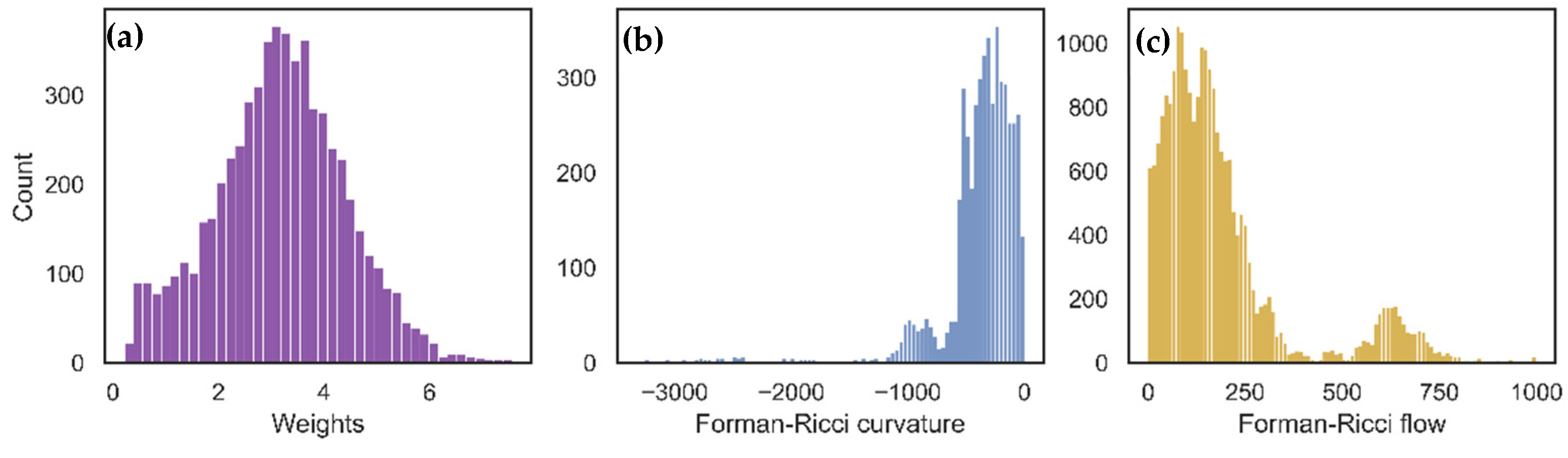
The aim of this section is to illustrate the process of Forman–Ricci flow by describing the evolution of the metric as a function of Forman–Ricci curvature. Ricci flow changes the metric such that regions with negative Ricci curvature expand and regions with positive Ricci curvature shrink.

The analysis was conducted on the semantic network described in Section 1. The edge weights were defined by the “distance function” mentioned above, which includes the two free parameters of minimum subjects per edge (MS) and window size (WS), or the maximum number of words that determine the distance between a given pair of words. For the purpose of describing Forman–Ricci flow, we selected parameters WS = 7 and MS = 10. Note that for any graph constructed from any parameters WS and MS, the direction of the effect between Forman curvature and the change in the metric are the same. In addition, we ran 20 iterations of Forman–Ricci flow (Formula 4) when the learning rate was 0.001. See Figure 1 for the distribution of Forman–Ricci curvature and the weights before and after Forman–Ricci flow. 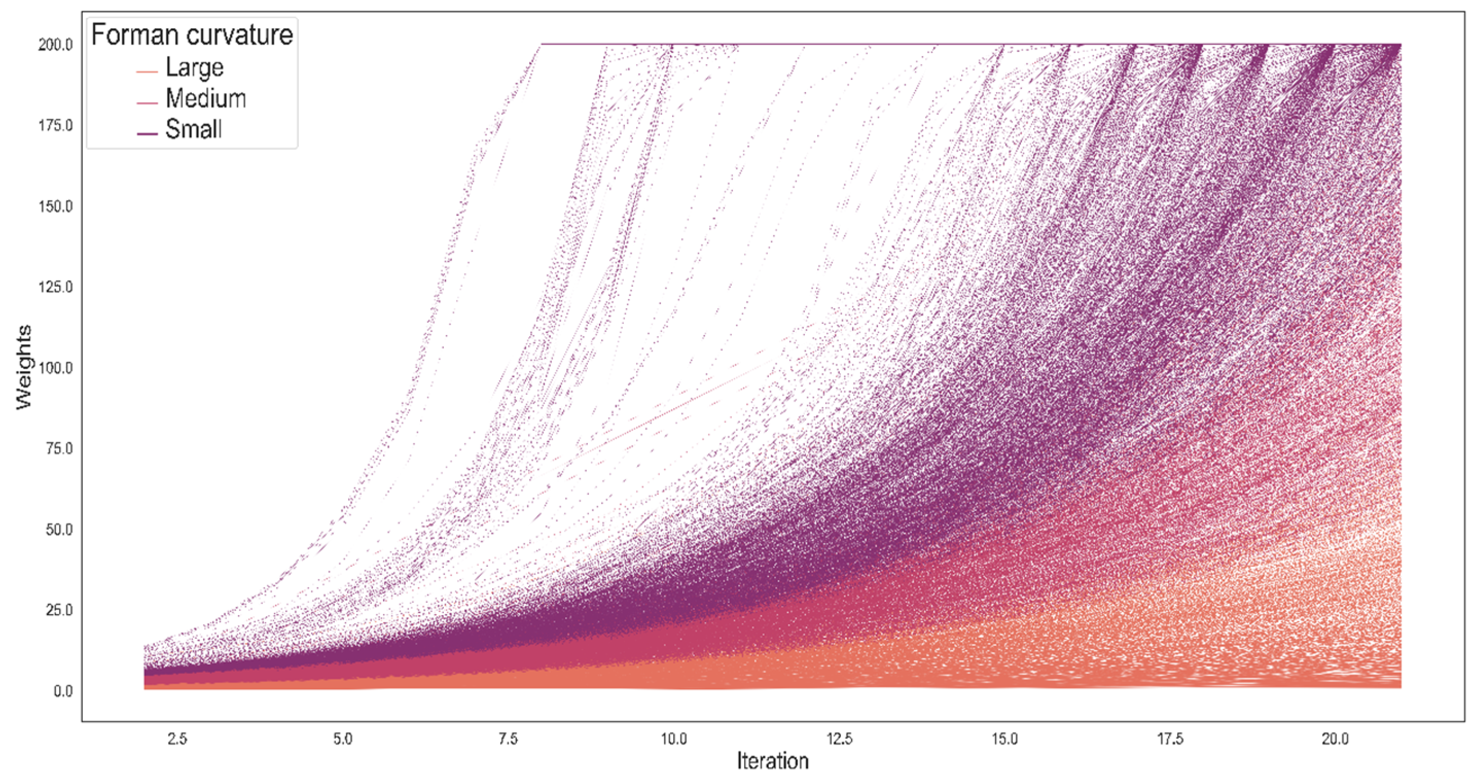Figure 2 illustrates the evolution of the graph as a function of Forman–Ricci curvature such that the greater the curvature of an edge, the higher the edge weight in the following Ricci flow iteration.

Figure 2 illustrates the fundamental relationship between Forman curvature at time t and the weight at time t + 1. A negative Forman curvature entails greater weights, while a positive Forman curvature entails smaller weights. The free parameters of the function that determines the weights affect the robustness of the graph and the temporal resolution of the weights: MS indicates the minimum number of people who moved from i to j, and the larger the WS, the more the weight from i to j can be based on relationships that contain a greater number of objects between them. It turns out that choosing other parameters for WS and MS changes the starting point of the analysis by establishing a different set of weights, but such a choice does not change the fundamental relationship between the curvature and the weight.

Our approach relies on the notion of Ricci flow in order to detect the core structure of the network. Consistent with Ni, Lin, Luo, and Gao [13], in a graph G in which the vertices are well connected such that the edges have positive curvature, then the structure of G after a number of iterations of Ricci flow is spherical. If the edges have negative curvature, then the structure of G after a number of iterations of Ricci flow is tree-shaped. As a result, in a graph that features areas with dense negative curvature surrounded by other areas containing edges with negative curvature, we find a division into communities

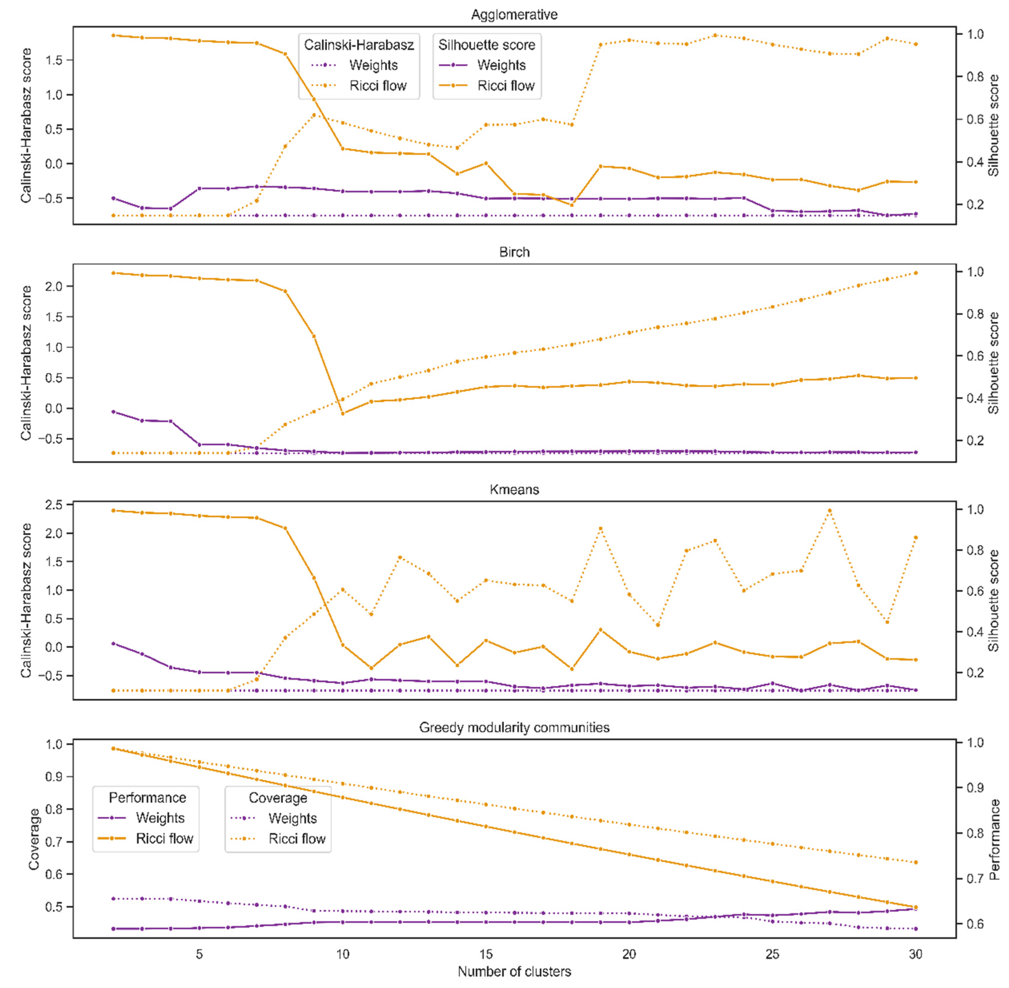
To estimate the effect of Forman–Ricci flow on the network structure, particularly the extent to which G is distributed to dense communities, we compare the network’s internal validity before and after calculating Forman–Ricci flow. Internal validity refers to the process of evaluating the quality of a clustering structure without referring to external information. Note that we use an internal validity approach because there is no ground truth.

We conducted the comparison between the internal validity of graph weights and the Forman–Ricci flow metrics as follows. First, for each set of weights, we initialized four different lists of clusters given by agglomerative, Birch, K-means, and greedy modularity communities on a range of a number of communities (2, 3, …, 30). Then, for each list of clusters and number of clusters, we computed internal validity with two different measures, Silhouette and Calinski–Harabasz scores. For greedy modularity communities, we computed internal validity by coverage and performance, with a high score indicating dense and well-separated communities. We anticipated that the Forman–Ricci flow process would increase the internal validation of the graph since, in the iterative process, we expected the metric to change so that the graph would split into more distinct communities than at the outset. We performed the analysis via the Scikit-learn package in Python [27]. For more details regarding the cluster algorithms and the internal validity measures, see Appendix A.

The results indicate that for the Calinski–Harabasz score, Ricci flow yields better results in all cases. For the Silhouette score, Ricci flow was better for all cases in Birch and for 28 out of 29 in agglomerative and K-means. In all cases, Ricci flow yields better results for coverage and performance scores (Figure 3). All told, the Forman–Ricci flow metric yields a better clustering performance than graph weights.

3.2. Object-Based Dynamic Measure

Here, we introduce our novel measure based on Forman–Ricci flow. This measure is applicable to many contexts, but to illustrate its use, we focus on the way it can quantify the impact of a word on semantic relations between other words.

To capture the object-based dynamic, we need to consider a multigraph $\widehat{G}=\left(V,E,w, I\right)$. A network is called a multigraph if a pair of vertices can be connected with multiple edges. The additional information $I$ is a class of disjointed sets, and in our case, $I$ is an ordered set of conditional event indexes: $I=\left\{{\left.\widehat{G}\right|}_s , {\left.\widehat{G}\right|}_{\neg s}\right\}$. That is, two graphs represent any object $s$, ${\left.\widehat{G}\right|}_s$ represents the weights between any two objects iff $s$ appears before the pair of objects, and ${\left.\widehat{G}\right|}_{\neg s}$ represent the weights between any two objects iff $s$ does not appear before the pair of objects.

Formally speaking, for $\widehat{G}=\left(V,E,w,I\right)$, we use the following steps to quantify the extent to which an object s changes the interactions between other objects:

1.

Define index $I$ for graph $\widehat{G}$ such that $I=\left\{{\left.\widehat{G}\right|}_s ,{\left.\widehat{G}\right|}_{\neg s}\right\},$ so that $s$ is represented by two graphs.

2.

For each element in $I$, define the weights for ${\left.\widehat{G}\right|}_s$ as $w_{ij}\in {\left.\widehat{G}\right|}_s:=w_{ij}|s_{i-k }$, for ${\left.\widehat{G}\right|}_{\neg s}$ as $w_{ij}\in , {\left.\widehat{G}\right|}_{\neg s}:=w_{ij}|\neg s_{i-k }$, for $k=1\cup 2$ and $j\le i+WS$.

3.

Compute steps 1–4 of the Forman–Ricci flow algorithm for each of the graphs $\left\{{\left.\widehat{G}\right|}_s ,{\left.\widehat{G}\right|}_{\neg s}\right\}$.

4.

For any $w_{ij}$ and $w_{ij}\in {\left.\widehat{G}\right|}_s$ and $w_{ij}\in {\left.\widehat{G}\right|}_{\neg s}$.

$$\delta \left(s\right)= \frac{1}{N}{\displaystyle \sum }_{w_{ij}\in {\left.\widehat{G}\right|}_s \mathrm{and} {\left.\widehat{G}\right|}_{\neg s}}{\left.\widehat{G}\right|}_s\left(w_{ij}\right)- {\left.\widehat{G}\right|}_{\neg s}\left(w_{ij}\right)$$

(5)

where N denotes the number of $w_{ij}$ that belongs to both graphs.

This object-based dynamic measure $\delta \left(s\right)$ can be used in two ways. The first, a directional approach, considers the direction of the effect. When an object that changes the weights is represented by a negative value, the structure is tree-like in the presence of s, meaning that the network conditional to s is significantly more diffuse than a network that is conditional to not s. When the object is represented by a positive value, the structure is spherical, meaning that the network conditional to s is more densely packed than a network that is conditional to not s. A value close to 0 indicates that there are no significant differences between the graphs. The second approach does not take direction into account. Instead, it considers the absolute value of $\delta \left(s\right)$, which represents the extent to which an object changes the metric in any direction. We examine both approaches in the next section, and we present descriptive analyses regarding $\delta \left(s\right)$ in Appendix A. The significant difference between the two measures is that in the directed version, a high value indicates a spherical-like structure, while a low value indicates a tree-like structure. The non-directed measure answers the fundamental question of whether the object affects the metric: a low value indicates no effect, and a high value indicates an effect.

By considering both measures, it is possible to check whether existing measures establish a correlation with spherical-like or tree-like structures or with the degree of influence of an object on the metric.

3.2.1. Study Case

Attention to the ever-changing nature of the semantic network has recently gained momentum [28,29], and here we demonstrate the application of our novel measure to this new perspective. In the context of an ongoing semantic retrieval task, we use our object-based dynamic measure to assess the impact of a word S on the interactions between the words that follow. By comparing the structure of the Ricci flow metric in a network that is conditioned by the utterance of the word S to the structure of the Ricci flow metric in a network that is conditioned by not S, we can identify the impact of S on the interactions between the following words. In the following sections, we show that certain sets of objects significantly change the metric; we examine both the directional and nondirectional approaches and compare those approaches with measures that already exist.

3.2.2. Analysis

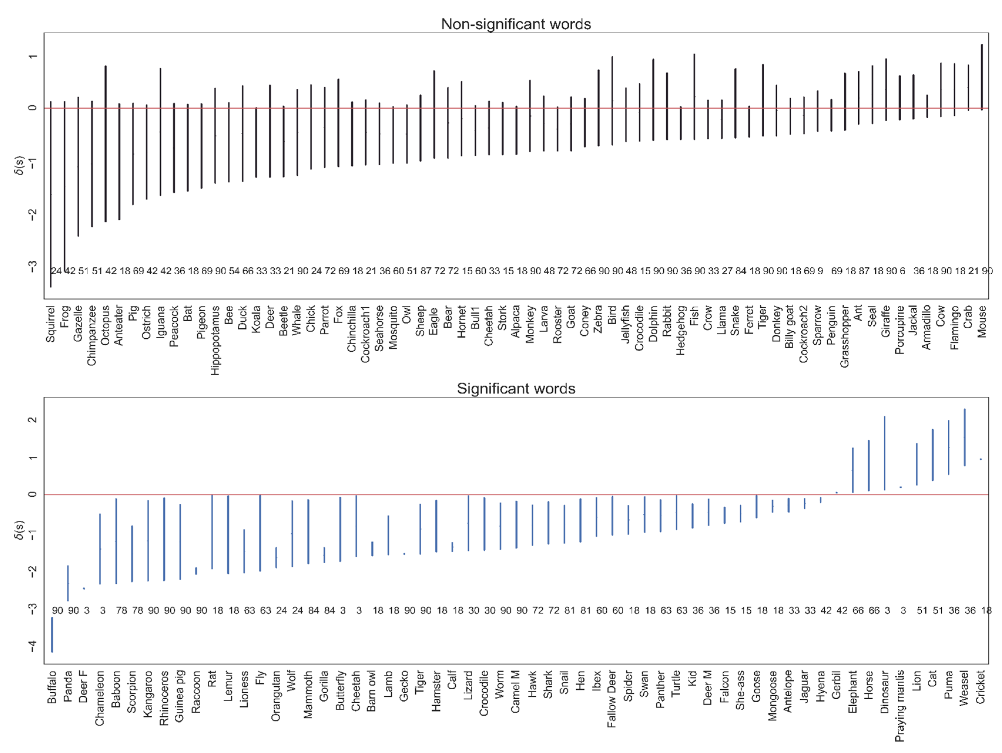
Our analysis aims to distinguish between the set of words that significantly affect the metric and the set of words that do not. To make this distinction, we assigned each word an object-based dynamic score given by $\delta \left(s\right)$ for any possible combination between the free parameters WS = (2,4,5,6,8,9) and MS = (3,5,7,9,15), the number of iterations of Forman–Ricci flow = (3,4,5), and a learning rate of 0.001. We based the score on 90 different networks to estimate the result’s stability for weights at different degrees of locality (WS) and power (MS and number of iterations). Finally, we performed a bootstrap test for each word to assess whether that word significantly changed the metric. The bootstrap was performed on the list of values in which the word received a $\delta \left(s\right)$ value (see Figure 4), when in each iteration (number of iterations = 10,000), the mean of a mini-batch $\left(\mathrm{N} = 5\right)$ was computed. Then, each word was bounded between the upper and lower numbers given by 10,000 mini-batch means, where the boundaries were corrected for multiple compressions via the Bonferroni correction, such that the lower boundary was $2.5/\mathrm{l}$ and the upper boundary $100-\left(2.5/\mathrm{l}\right)$, with $\mathrm{l} = 130$, representing the number of compressions. Finally, if the value 0 was not included in the boundaries, we determined that the word’s effect on the metric was significantly different from 0; otherwise, we determined that the result was non-significant.

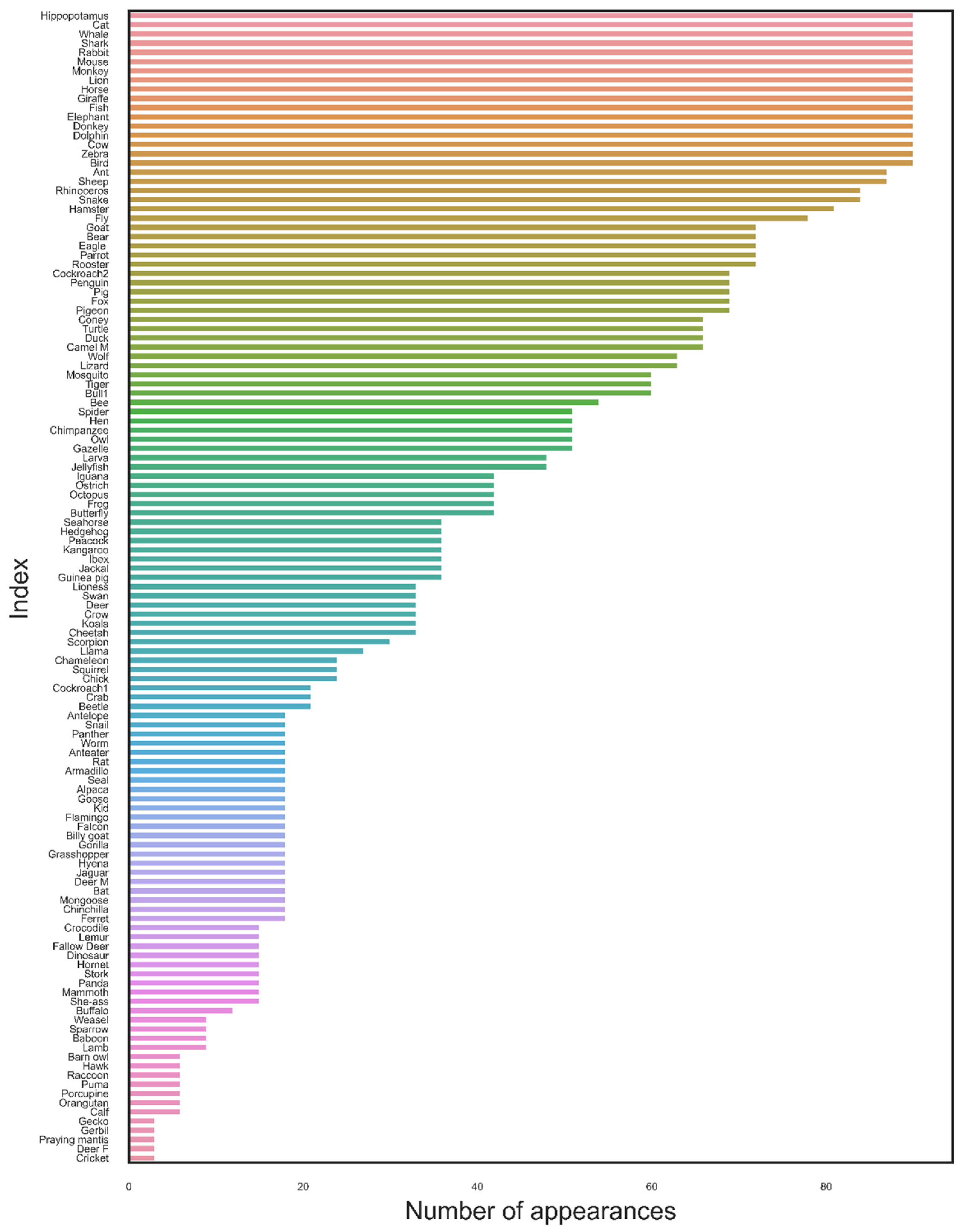
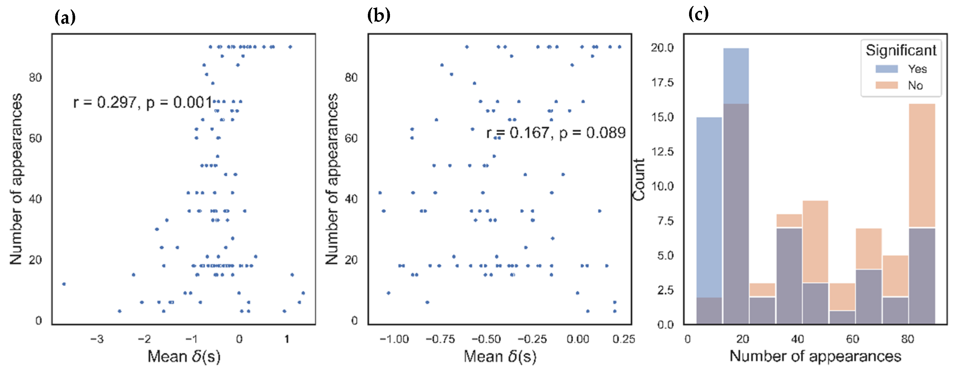
In sum, out of 130 words, 61 significantly changed the network structure, and 69 were non-significant (Figure 5). Additionally, in most cases, the words had small $\delta \left(s\right)$ values, which made the network structure more tree-like than it would have been in the absence of those words. We will include a comprehensive discussion about the direction of a word’s effect (tree-like or spherical) in a follow-up study. Additional analyses can be found in the appendix.

3.3. Exploratory Comparison Analysis

To determine whether our object-based dynamic measure, $\delta \left(s\right)$, contributes new information, this section will compare $\delta \left(s\right)$ with already existing measures. We will examine both the directional and nondirectional approaches and compare them with centrality measures, scalar curvature measures, and word frequency and location. We will see whether the effect of an object on its environment, as measured in the object-based dynamic, is reflected in those alternative measures.

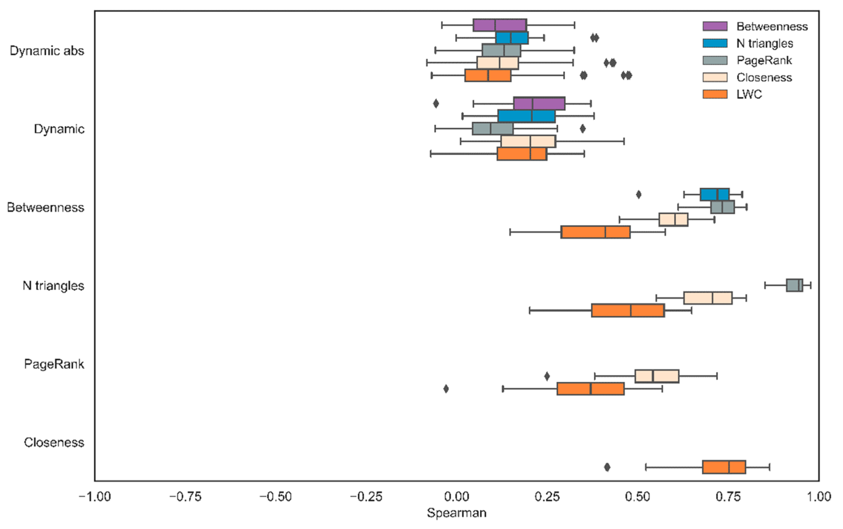
3.3.1. Centrality Measures

Centrality measures capture how a vertex influences the flow of information in the network, and in this section, we focus on two sets of this type of measure. The first set, which captures how close a vertex is to other objects, includes the number of triangles, closeness, and PageRank. The second set, which captures how a word functions as an intermediary, includes betweenness and LDC. We will examine empirically the extent to which $\delta \left(s\right)$ differs from all these other measures, but we must first introduce the measures:

• The number of triangles: This measure calculates the number of undirected three-cliques for each vertex in the graph. The number of triangles is used to detect vertices that belong to numerous cliques. It is worth noting that this measure is closely related to the clustering coefficient.
• Closeness: This measure is the inverse of farness, which is defined as the mean of the shortest paths to all other vertices [30,31]. Closeness can be interpreted as the expected time of arriving at a word through the graph’s shortest paths. The gist of this metric is to assign more importance to the vertices that are closest. The definition is as follows:

  $$C\left(v\right)= \frac{N-1}{ {{\displaystyle \sum }}_u\delta \left(v,u\right)}$$

  (6)

  where $\delta \left(v,u\right)$ represents the length of the shortest path between $v$ and $u$. This measure takes weight into account by averaging the shortest paths that emerge from $v$.
• PageRank: The basic idea of the PageRank algorithm, first introduced in a Google paper [32], is that a central vertex is determined not only by the number of incoming edges (in-degree) but also by the level of importance of the incoming vertices. T represents the set of vertices, $N_u$ represents the number of vertices to which vertex v points, and ${\mathrm{S}}_V$ represents the set of vertices pointing to vertex v. Finally, $\alpha$ is the damping factor of the probability of jumping from a given vertex to another random vertex in the graph. PageRank is computed as follows:

  $$\mathrm{PR}\left(\mathrm{v}\right)= {\displaystyle \sum }_{u\in S_V}\frac{PR\left(u\right)}{N_u}+\frac{1-\alpha }{T}$$

  (7)
• Betweenness: This measure was introduced by Freeman [33] in order to quantify the extent to which a vertex tends to be on the shortest paths between other vertices—in other words, to serve as an intermediary. Betweenness for a vertex v is defined as follows:

  $$\mathsf{\gamma }\left(v\right)={\displaystyle \sum }_{i\ne v\ne j\in V}\frac{{\sigma }_{ij}\left(v\right)}{{\sigma }_{ij}}$$

  (8)

  where ${\sigma }_{ij}\left(v\right)$ represents the number of shortest paths between i and j that go through v, and ${\sigma }_{ij}$ represents the total number of shortest paths between i and j.
• LDC: In Cohen et al. [34], we recently proposed local detour centrality (LDC), a novel centrality measure for weighted and directed graphs that quantifies the tendency of a given vertex to lie on the shortest possible path between other vertices. In other words, LDC indicates whether the possible path between $v_1$ and $v_2$ is significantly closer when $v$ lies between them, in contrast to cases in which $v$ does not lie between them. Let $G=\left(V,E\right)$ be an edge-weighted and directed graph in which $w\left(v_{\mathrm{i}},v_{\mathrm{j}}\right)$ represents the weights from $v_{\mathrm{i}}$ to $v_{\mathrm{j}}$ and let $\delta \left(v_{\mathrm{i}},v_{\mathrm{j}}\right)$ denote the shortest path from $v_{\mathrm{i}}$ to $v_{\mathrm{j}}$ based on Dijkstra’s shortest path algorithm. For any vertex $v$,
  • Let $L= \left\{v_1,v_2\dots v_n\right\}$ such that any $v_{\mathrm{i}} \in L$ if $\delta \left(v,v_{\mathrm{i}}\right) \le r$ or $\delta \left(v_{\mathrm{i}},v\right)\le r$. The number $r = \frac{1}{\left|\mathrm{V} \left(G\right)\right|}{\displaystyle \sum }_{v_{i, }{v}_{j }\in V}\delta \left(v_i,v_j\right)$ is called the threshold.
  • Let $G_v\subset G$ be a complete graph with $V\left(G_v\right) = L$ where, in this case, $w\left(v_i,v_j\right)=\delta \left(v_{\mathrm{i}},v_{\mathrm{j}}\right)$.

To calculate local intermediateness, for any vertex $v$, let us first introduce some further notations:

Let $GN=\left(V,E\right)$ be the complete graph, where the weights are calculated according to the Dijkstra’s shortest path algorithm on the following weights:

$$w^{\prime }\left(v_i,v_j\right)=\left\{\begin{array}{cc}{\max }_{v_{k, }{v}_{l }\in V}\left(w\left(v_{\mathrm{k}},v_{\mathrm{l}}\right)\right)& v_j=v or v_i=v\\ w\left(v_i,v_j\right)& otherwise\end{array}\right.$$

Since both graphs $G_{\overline{v}}$, $G_v$ have the same edges but not the same weights, we denote E’ = E($G_{\overline{v}}$) = E($G_v$). Then, the local detour centrality (LDC) of the vertex $v$ is defined as follows:

$$LDC\left(v\right)= \frac{1}{\left|L\right|}{\displaystyle \sum }_{e \in E^{\prime } }\left(G_{\overline{v}}{}_e–G_v{}_e\right)$$

(9)

Analysis: In sum, centrality measures capture the extent to which a vertex dictates the flow of information in a static graph. Here, we examine whether centrality computed in a static graph encodes information about changes to the metric over time.

For any possible combination between the free parameters WS (window size), comprising the values (2,4,5,6,8,9); MS (minimum subjects per edge), comprising the values (3,5,7,9,15); the number of iterations of Forman–Ricci flow = (3,4,5); and a learning rate of Ricci flow algorithm at 0.001, each word received a list of values given by the object-based dynamic scores $\delta \left(s\right)$ and |$\delta \left(s\right)$| as well as each centrality measure described above. We based the score on 90 different networks so that we could estimate the stability of the result for weights at different degrees of locality (WS) and power (MS and number of iterations).

For the directional approach, the mean correlation between $\delta \left(s\right)$ and the alternative centrality measures were as follows: number of triangles (M = 0.19, SD = 0.1), PageRank (M = 0.1, SD = 0.1), closeness (M = 0.2, SD = 0.1), betweenness (M = 0.2, SD = 0.1), and LDC (M = 0.17, SD = 0.1). For the nondirectional approach, the mean correlation between the absolute value $\delta \left(s\right)$ and the alternative centrality measures were as follows: number of triangles (M = 0.15, SD = 0.07), PageRank (M = 0.13, SD = 0.08), closeness (M = 0.12, SD = 0.1), betweenness (M = 0.11, SD = 0.09), and LDC (M = 0.11, SD = 0.13) (Figure 5).

All in all, we found a high correlation among centrality measures but a weak correlation between those measures and the object-based dynamic score. In comparison with the nondirectional approach, the directional approach yielded a slightly higher correlation to the alternative centrality measures.

3.3.2. Scalar Curvature

As we have already mentioned, Ricci curvature is classically defined on smooth manifolds and measures the deviation of the manifold from being locally Euclidean in various tangential directions. Ricci curvature is an edge-based measure defined by averaging all sectional curvatures of the planes where the edge is present. The measure captures two essential geometric properties: the growth of volume and the dispersion of geodesics. As a result, Ricci-curvature provides insight into the local geometric properties near the edge as well as the topological structure of the network. Scalar-curvature is a vertex measure that is calculated by averaging all Ricci curvatures in all directions in which the vertex appears. One might therefore expect Scalar curvature to capture local temporal changes in the network. In this section, we compare both object-based dynamic $\delta \left(s\right)$ and |$\delta \left(s\right)$| to different discretizations of Ricci-curvature: Menger, 1-dimensional Forman, 2-dimensional Forman, and Haantjes.

Our analysis did not include Ollivier-Ricci curvature [35] because of its computational complexity compared to other measures and because of its metric assumptions; by contrast, we calculate the curvature directly on the weights. Since previous studies have shown that Ollivier-Ricci curvature maintains a high correlation with Forman–Ricci curvature in many networks [15], we have found it sufficient to focus on two different perspectives of Forman–Ricci curvature in this framework.

1.

Haantjes curvature: This curvature [36] is a path-based measure and can be generalized to a path of length $n$ by replacing path ab ∪ bc with a path of length $n$. For a general discrete notion of Haantjes curvature, let $\pi =\left(v_0,\dots ,v_n\right)$ be a directed path between the vertices $v_0$ and $v_n$. The simplified Haantjes-Ricci curvature of the path $\pi$ is then defined as follows [37]:

$${\kappa }_H^2\left(\pi \right)=\frac{l\left(\pi \right)-d\left(v_0, v_n\right)}{d\left(v_0, v_n\right)}$$

(10)

Next, the Haantjes-scalar curvature of $v$ in $G$ is defined as follows:

$$\kappa s_H^2\left(v\right) = {\displaystyle \sum }_{\pi ~ v}{\kappa }_H^2\left(\pi \right)$$

(11)

where $\pi ~ v$ denotes the paths that are anchored to vertex $v$. Note that while Menger-Ricci and Forman–Ricci take into account only triangles or simple paths of length 2, Haantjes-Ricci considers paths of any length; in this study, however, we limit the analysis to triangles because of computational considerations. The resulting simplicial complexes are canonical geometric structures that are commonly used to model higher-order correlations in networks.

2.

Menger–Ricci curvature: In 1930 Menger introduced a discrete definition of Ricci curvature K(T) for any three vertices in the network. Let (M, d) be a metric space and T = T(a, b, c) be a triangle with sides lengths a, b, c, and denote $p = \frac{a+b+c}{2}$. Then the Menger curvature of T is given by

$$K_m\left(T\right)= \frac{\sqrt{p\left(p-a\right)\left(p-b\right)\left(p-c\right)}}{abc}$$

(12)

The Menger–Ricci curvature of a vertex e in a network can be defined as

$$K_m\left(v\right)={\displaystyle \sum }_{T_e~ v}{K}_m\left(e\right)$$

(13)

where T_e ∼ e denotes the triangles adjacent to the vertex v. Intuitively, if an edge is part of several triangles in the network, that edge will have a high positive Menger-Ricci curvature.

Note that the definition of Menger-Ricci in (12) relies on the geometry of the Euclidian plane. This geometric assumption is incorrect in many cases, however, including hyperbolic spaces [14]. By contrast with Menger-Ricci curvature, Haantjes and Forman–Ricci curvatures do not assume any background geometry.

3.

Forman–Ricci curvature: There are different ways to calculate Forman–Ricci curvature of a directed and weighted network. Formula (1) described 1-dimensional Forman–Ricci curvature, and here we present an extension by Saucan, Sreejith, Vivek-Ananth, Jost, and Samal [16], the 2-dimensional Augmented Forman–Ricci curvature (AFR). FR1 considers only the pairwise correlation between vertices; while computing FR1 for the directed edge $e =\left(v_1,v_2\right)$, we consider only the incoming edges to $v_1$ and the outcoming edges from $v_2$. 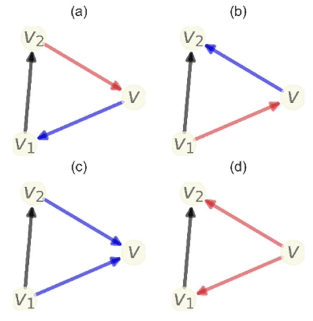By contrast, AFR considers 2-dimensional faces—cases in which three vertices form a triangle—and potentially higher-order faces as well. Although there are four different types of directed triangles, we consider only two types (see Figure 6). The directed triangular face t formed by vertices ($v_1,v_2,v_3)$ and edges {($v_1,v_2),\left(v_2,v_3\right),\left(v_3,v_1\right)\}$ makes a positive contribution. In this case, since the information from $v_3$ “flows” back to $v_1$, the triangle represents a spherical structure that is consistent with the interpretation of a positive Forman–Ricci curvature. The directed triangular face t formed by edges {($v_1,v_2),\left(v_1,v_3\right),\left(v_3,v_2\right)\}$ makes a negative contribution. This triangle represents a tree-like structure since the information “flows” out from vertex $v_1$ to vertex $v_2$ and so also from vertex $v_1$ to $v_3$ and from there to $v_2$.

The augmented Forman–Ricci curvature $AFR\left(e\right)$ in a directed and weighted graph is given by the following equation:

$$AFR\left(e\right)=w_e\left({\displaystyle \sum }_{e<t}\frac{w_e}{w_t}+\left(\frac{w_{v_1}}{w_e}+\frac{w_{v_2}}{w_e}\right)\right)-{\displaystyle \sum }_{e_{I,v_1},e_{O,v_2}~e,e_{I,v_1},e_{O,v_2}\nless t}\left(\frac{w_{v_1}}{\sqrt{w_e{w}_{e_{I,v_1}}}}+\frac{w_{v_2}}{\sqrt{w_e{w}_{e_{O,v_2}}}}\right)$$

(14)

Here w_t denotes the weight of face t, and σ < τ means that σ is a face of τ. The augmented Forma–Ricci curvature of a vertex v in a network can be defined as

$$AFR\left(v\right)={\displaystyle \sum }_{T_e~ v}FR1\left(e\right)$$

(15)

Note that in order to calculate $\kappa s_H^2$, $K_m\left(v\right), FR1\left(v\right)$ and $AFR\left(v\right)$ in all of our statistical analyses, we use the median and not the sum for statistical reasons.

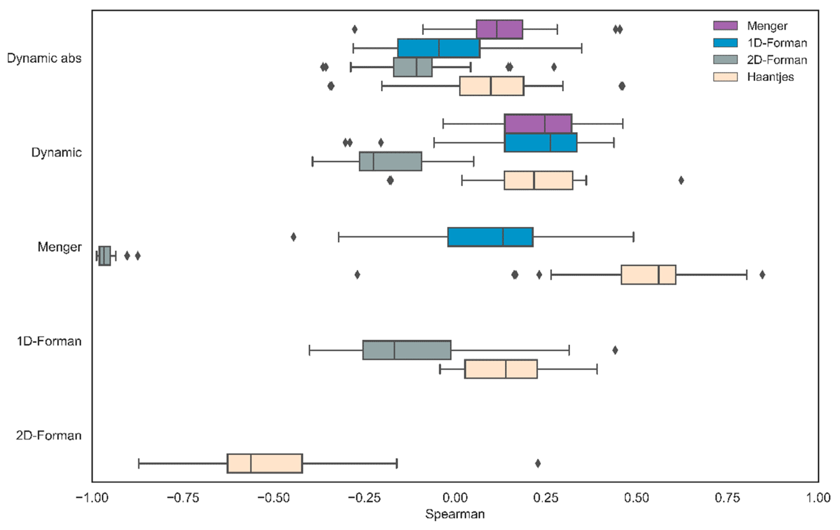
Analysis: As we did in our previous analysis, we constructed 90 networks based on the different possible combinations of the free parameters WS, MS, and number of iterations. For the directional approach, the mean correlation between $\delta \left(s\right)$ and the alternative scalar curvature measures were as follows: Haantjes [M = 0.21, SD = 0.14], Menger [M = 0.22, SD = 0.12], 1D-Forman [M = 0.21, SD = 0.17]. and 2D-Forman [M = −0.18, SD = 0.12]. For the nondirectional approach, the mean correlation between the absolute value $\delta \left(s\right)$ and the alternative scalar curvature measures were as follows: Haantjes [M = 0.09, SD = 0.15], Menger [M = 0.11, SD = 0.12], 1D-Forman [M = −0.02, SD = 0.16] and 2D-Forman [M = −0.1, SD = 0.12] (Figure 7).

In sum, we found a low degree of correlation between the object-based dynamic score and the different discretizations of scalar curvature for both approaches. The directional approach correlates with the alternative scalar curvature measures more closely than the nondirectional approach, and this result is consistent with our previous analysis. In addition, we found a nontrivial and high degree of correlation between Menger–Ricci curvature and 2-dimensional Forman–Ricci curvature. This observation is highly relevant since it shows that for all practical purposes, the elementary Menger curvature and the far less intuitive 2-dimensional Forman–Ricci curvature essentially coincide. This coincidence demonstrates that the combinatorically defined Forman curvature also captures the essential geometry of the underlying simplicial complex.

3.3.3. Frequency and Word Location

Word frequency effects are manifested in many ways, including lexical access [38], lexical decision-making [39], perceptual identification [40], and recall [41]. In addition, word frequency is strongly related to lexical similarity, so word frequency reflects the strength of the connection to other words [42]. The effect of word frequency on access and similarity raises the possibility that word frequency influences the upcoming semantic interactions. Furthermore, in a serial search, word location is negatively correlated with log-frequency [43,44]. Another measure that is closely related to word frequency is degree centrality. 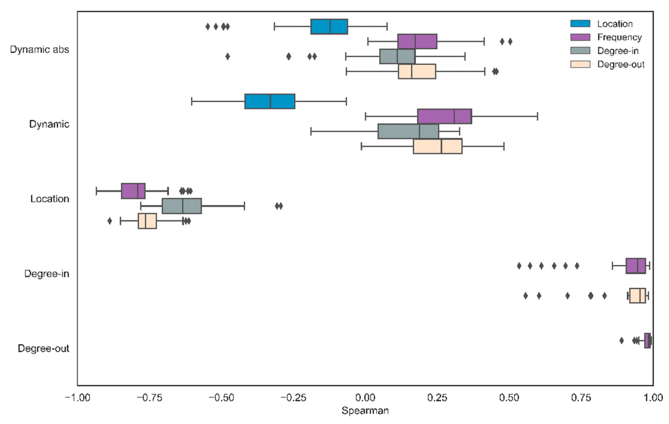For a directed graph $G$ and the vertex $v ϵ V$, the in-degree of vertex v refers to the number of arcs that incident from v, and the out-degree refers to the number of arcs that incident to v. As will be shown below, word frequency is strongly correlated with degree distribution. Given all these considerations, in this analysis, we examine three strongly related but dissimilar measures—frequency, location, and degree centrality—and test the correlation between each of them and our object-based dynamic measure.

Analysis: As in our previous analyses, we constructed 90 networks based on the different possible combinations of the free parameters WS, MS, and number of iterations. For the directional approach, these were the mean correlations between $\delta \left(s\right)$ and each measure: log-frequency (M = 0.28, SD = 0.14), average location (M = −0.33, SD = 0.14), degree-in (M = 0.15, SD = 0.12), and degree-out (M = 0.24, SD = 0.12). For the nondirectional approach, the mean correlations between absolute $\delta \left(s\right)$ and each measure were as follows: log-frequency (M = 0.19, SD = 0.11 ), average location (M = −0.14, SD = 0.12), degree-in (M = 0.08, SD = 0.15), and degree-out (M = 0.17, SD = 0.11) (Figure 8).

In sum, the correlation with log-frequency, degree-in, and degree-out is low for both directional and non-directional approaches. We found the strongest connection between the directed approach and word location; words that change their environment tend to appear at the beginning of the task. By contrast, the correlation among log-frequency, word location, degree-in, and degree-out was near perfect.

4. Discussion

The explosion of big data increasingly includes temporal information, which plays a central role in shaping network structure. This study attempts to include temporal information in network analysis by shifting from a static to a temporal perspective. We present our object-based dynamic approach, which investigates the extent to which an object that is represented in the network by a vertex affects the network’s topology over time. We explore how the presence of an object may affect subsequent interactions between other objects, leading to topological changes in the network.

By combining tools from complex networks and differential geometry, we can present a fine-grained description of the object-based dynamic approach, an approach that enables us, like other researchers who have combined the same tools, to study applied problems [45,46,47]. The use of multigraphs provides a useful representation of network evolution, with each set of edges representing a distinct and discrete event in the flow of information over time. In our case, each object receives two sets of edges, one expressing the interactions conditional to the presence of another specific object, and the other expressing the interactions conditional to that object’s absence. With these two sets of edges, we can investigate whether the object’s direction affects the shape of the network. To do this, we implement Forman–Ricci flow separately to each set, aiming for a regularization effect for each set of edges and a revelation of their core topology. By allowing us to compare the geometry of the two sets, this process enables us to determine the impact of an object’s presence.

The main advantage of our measure is that it does not estimate the relative contribution of a vertex for a given set of weights, as can be done using various graph measures. Instead, the estimation is based on a comparison between two sets of weights, which makes it possible to examine the degree of influence of an object over time. Since the measure is object- rather than vertex-based, it does not represent a property of a vertex in the graph, and as a result, it cannot be used in the context of a structural analysis of the graph. It functions instead as a comparative measure between objects, shedding light on the direction and strength of an object’s influence on the relationships between other objects. As a result, one can distinguish between centrality measures and object-based dynamic measures. Centrality measures examine the connections that pass through, enter, or exit a given vertex in a graph with a defined set of weights. Here, we estimate the impact of a chosen object by comparing it to distinct sets of weights, the weights conditional to its presence and the weights conditional to its absence.

This comparative feature of our object-based approach makes it applicable to the analysis of social networks. To this aim, one might build two graphs for each person, with one graph representing the social interactions among other people given that person’s presence, and the other graph representing the social interactions among the same set of people given that person’s absence. By comparing the graphs, it would be possible to examine to what extent that person influences social relations. Here, a major constraint is the need for serial data in the construction of networks. The effect of the chosen person on the group can be examined only if we compare the social interactions that follow the person’s specific contribution to the social interactions that take place without that previous contribution. Data that would enable such a comparison include timestamped posts or responses in a social network; these would allow the researcher to see how the group’s interactions after that person’s input compared to the group’s interactions after other people’s input.

Our own context, however, is the semantic network. More specifically, we assess the impact of a word retrieved from memory on the subsequent words that the agent retrieves. Our purpose is to describe the effect of Forman–Ricci flow as a regularization term on the weights. The networks achieved with and without the use of this Forman–Ricci flow are significantly different on various internal validity scores; after regularization, the network cluster topology is much more defined. This finding is consistent with Ni, Lin, Luo, and Gao [13], but they use Ollivier curvature and not Forman curvature as we do. Another of our goals is to uncover the set of words whose presence significantly changes the topology. Finally, we examine whether the temporal perspective represented by our object-based dynamic indeed contributes new information beyond that provided by existing measures that are based on a static graph. At least for the empirical data provided by the retrieval task, we demonstrate that centrality measures, scalar curvature measures, word location, and frequency are poorly correlated with the object-based dynamic score.

A potential follow-up study might examine the differences between Ricci flow based on 1-dimensional Forman curvature and Ricci flow based on 2-dimensional Forman curvature. This research might investigate the differences in the speed with which the graph is characterized by singularity and the creation of a network characterized by well-defined, distinct communities.

In the context of a semantic network, our object-based measure both resembles and differs from the work of Nachshon, Cohen, and Maril [21], which demonstrates how a specific word might influence relations between other words. Their demonstration considers all the triplets (A,B,C) that violate the triangle inequality assumption (AB + BC ≥ AC). By replacing AC with the conditional edge BC preceded by A, one can assess whether the conditional edge will continue to violate triangle inequality. This approach, like ours, investigates the impact of an object on other interactions. However, while Nachshon, Cohen, and Maril examine local influence, a single edge at a time, this paper takes a global approach, building a whole new network to examine an object’s influence on the network’s structure. Further investigation will examine the fundamental difference between words that affect the metric and words that do not, and then take up the difference between words whose presence creates a tree-like space and words whose presence creates a spherical space.